The arithmetic-geometric scaling spectrum for continued fractions

Abstract.

To compare continued fraction digits with the denominators of the corresponding approximants we introduce the arithmetic-geometric scaling. We will completely determine its multifractal spectrum by means of a number theoretical free energy function and show that the Hausdorff dimension of sets consisting of irrationals with the same scaling exponent coincides with the Legendre transform of this free energy function. Furthermore, we identify the asymptotic of the local behaviour of the spectrum at the right boundary point and discuss a connection to the set of irrationals with continued fraction digits exceeding a given number which tends to infinity.

1. Introduction and statement of results

Many ergodic and dynamical properties of the Gauss map

(1.1) $$T\colon\mathbb{I}\to\mathbb{I},\>x\mapsto\frac{1}{x}-\left\lfloor\frac{1}{x}\right\rfloor,$$

where $\mathbb{I}:=\left(0,1\right)\setminus\mathbb{Q}$, have been studied in great detail (e.g. [Kuz28, Wir74]). Also its close relation to the Riemann $\zeta$-function via its Mellin transform is well-known, i.e. $\zeta\left(s\right)-1=\left(s-1\right)^{-1}-s\int_{0}^{1}T\left(x\right)x^{s-1}\,dx$. From the ergodic theoretical point of view the Gauss map reflects mainly geometric features of continued fraction expansion, whereas the Riemann $\zeta$-function reflects important arithmetic properties. In this paper we establish an approach to quantify the difference of these two aspects. For this let us begin with some elementary observations.

Every $x\in\mathbb{I}$ has a unique representation by its regular continued fraction expansion, i.e. we have a bijective map $\pi\colon\mathbb{I}\longrightarrow\mathbb{N}^{\mathbb{N}}$, where $\pi\left(x\right)=\left(a_{i}\left(x\right)\right)_{i\in\mathbb{N}}$ with

$$x=\cfrac{1}{a_{1}\left(x\right)+\cfrac{1}{a_{2}\left(x\right)+\cfrac{1}{a_{3}\left(x\right)+\cdots}}}.$$

For $n\in\mathbb{N}$ the $n$-th convergent of $x\in\mathbb{I}$ is given by the reduced fraction

$$\frac{p_{n}\left(x\right)}{q_{n}\left(x\right)}:=\cfrac{1}{a_{1}\left(x\right)+\cfrac{1}{\ddots+\cfrac{1}{a_{n-1}\left(x\right)+\cfrac{1}{a_{n}\left(x\right)}}}},$$

which is uniquely determined by the first $n$ digits of its continued fraction expansion. Hence, we will also use the notation $q_{n}\left(\omega\right):=q_{n}\left(x\right)$ and $p_{n}\left(\omega\right):=p_{n}\left(x\right)$ whenever $\omega$ is an infinite or finite word of length at least $n$ over the alphabet $\mathbb{N}$ such that the vector of the first $n$ entries coincide with $\left(a_{1}\left(x\right),\ldots,a_{n}\left(x\right)\right)$. For the denominator we then have the following recursive formula

(1.2) $$q_{n}\left(x\right) = a_{n}\left(x\right)q_{n-1}\left(x\right)+q_{n-2}\left(x\right),$$

with $q_{-1}=0$ and $q_{0}=1$. From this one immediately verifies that

(1.3) $$\prod_{i=1}^{n}a_{i}\left(x\right)\leq q_{n}\left(x\right)\leq 2^{n}\prod_{i=1}^{n}a_{i}\left(x\right),$$

showing that the arithmetic expression $\prod_{i=1}^{n}a_{i}\left(x\right)$ does not differ too much from the geometric term $q_{n}\left(x\right)$. Yet, the two terms may grow on different exponential scales. Our main aim is to investigate the fluctuation of the asymptotic exponential scaling. For this let us define the arithmetic-geometric scaling of $x\in\mathbb{I}$ by $\lim_{n\rightarrow\infty}\log\prod_{i=1}^{n}a_{i}\left(x\right)/\log q_{n}\left(x\right)$ if the limit exists. The fluctuation of this quantity is captured in the level sets

$$\mathcal{F}_{\alpha}:=\left\{x\in\mathbb{I}:\lim_{n\rightarrow\infty}\frac{\log\left(\prod_{i=1}^{n}a_{i}\left(x\right)\right)}{\log q_{n}\left(x\right)}=\alpha\right\}$$

for a prescribed scaling $\alpha\in\mathbb{R}$.

The following list of facts give a first impression of these level sets. Their proofs will be postponed until Subsection 2.3.

Fact 1.1.

For $\alpha\notin\left[0,1\right]$ we have $\mathcal{F}_{\alpha}=\emptyset$.

Fact 1.2.

The noble numbers (i.e. those numbers whose continued fraction expansion eventually contain only $1$’s) are contained in $\mathcal{F}_{0}$.

Fact 1.3.

For $k\in\mathbb{N}$ the quadratic surd $\pi^{-1}\left(k,k,\dots\right)$ lies in $\mathcal{F}_{\alpha\left(k\right)}$, where

$$\alpha\left(k\right):=\frac{\log k}{-\log\left(-k/2+\sqrt{k^{2}/4+1}\right)}\in[0,1)\textrm{ and }\lim_{k\rightarrow\infty}\alpha\left(k\right)=1.$$

Fact 1.4.

The numbers having a continued fraction expansion with digits tending to infinity are contained in $\mathcal{F}_{1}$, i.e. $\mathcal{G}:=\left\{x\in\mathbb{I}:a_{i}\left(x\right)\rightarrow\infty\right\}\subset\mathcal{F}_{1}$.

Fact 1.5.

We have for $\lambda$-almost every $x\in\left(0,1\right)$ that

$$\lim_{n\longrightarrow\infty}\frac{\log\prod_{i=1}^{n}a_{i}\left(x\right)}{\log q_{n}\left(x\right)}=\frac{12\log 2}{\pi^{2}}\log\left(K_{0}\right):=\alpha_{0}=0.8325\ldots,$$

where $\lambda$ denotes the Lebesgue measure restricted to $[0,1]$ and

$$K_{0}:=\prod_{k\in\mathbb{N}}\left(1+\left(k\left(k+2\right)\right)^{-1}\right)^{\log k/\log 2}$$

the Khintchin constant (cf. [Khi56]). Consequently, we have $\lambda\left(\mathcal{F}_{\alpha_{0}}\right)=1$.

Fact 1.6.

Also for later use let us define

$$\mathcal{F}_{\alpha}^{*}:=\begin{cases}\left\{x\in\mathbb{I}:\limsup_{n\rightarrow\infty}\log\left(\prod_{i=1}^{n}a_{i}\left(x\right)\right)/\log q_{n}\left(x\right)\geq\alpha\right\},&\alpha\geq\alpha_{0},\\ \left\{x\in\mathbb{I}:\liminf_{n\rightarrow\infty}\log\left(\prod_{i=1}^{n}a_{i}\left(x\right)\right)/\log q_{n}\left(x\right)\leq\alpha\right\},&\alpha<\alpha_{0}.\end{cases}$$

Then for $\alpha_{q}:=1-\left(q^{2}\log\left(q\right)\right)^{-1}$, $q>2$, we have

$$\mathcal{I}_{q}:=\left\{x\in\mathbb{I}:a_{i}\left(x\right)\geq q,\,i\in\mathbb{N}\right\}\subset\mathcal{F}_{\alpha_{q}}^{*}.$$

Fact 1.7.

For $x\in\mathcal{F}_{1}$ the sequence $\left(a_{i}\left(x\right)\right)$ is necessarily unbounded. This is to say that the set $\mathcal{F}_{1}$ is contained in the complement of the set $\mathcal{B}$ of badly approximable numbers.

The Hausdorff dimension $\dim_{H}\left(\mathcal{F}_{\alpha}\right)$ is an appropriate quantity to measure the size of the sets $\mathcal{F}_{\alpha}$. In this paper we will give a complete analysis of the arithmetic-geometric scaling spectrum

$$f\left(\alpha\right):=\dim_{H}\left(\mathcal{F}_{\alpha}\right),\qquad\alpha\in\mathbb{R}.$$

We already know from Fact 1.5 that the maximal Hausdorff dimension $f\left(\alpha\right)=1$ is attained for $\alpha=\alpha_{0}$ and $f$ is zero outside of $\left[0,1\right]$. Since the noble numbers have Hausdorff dimension zero there is some evidence that $f\left(0\right)=0$. In fact, both boundary points $0$ and $1$ will need some extra attention concerning this analysis.

Using the Thermodynamic Formalism we will be able to express the function $f$ on $[0,1]$ implicitly in terms of the arithmetic-geometric pressure function

$$P\left(t,\beta\right):=\lim_{n\rightarrow\infty}\frac{1}{n}\log\sum_{\omega\in\mathbb{N}^{n}}q_{n}\left(\omega\right)^{-2t}\prod_{i=1}^{n}\omega_{i}^{-2\beta},\quad t,\beta\in\mathbb{R},$$

We shall see in Lemma 2.1 that the limit defining $P$ always exists as an element of $\mathbb{R}\cup\left\{+\infty\right\}$. By Proposition 2.9 we have that for every $\beta\in\mathbb{R}$ there exists a unique number $t=t\left(\beta\right)$, such that $P\left(t\left(\beta\right),\beta\right)=0$. We denote by $\beta\mapsto t\left(\beta\right)$ the arithmetic-geometric free energy function (see Fig. 1.1). For any real convex function $g$ we let $\widehat{g}\colon\mathbb{R}\to\mathbb{R}\cup\left\{\infty\right\}$ denote the Legendre transform of $g$ given by $\widehat{g}\left(p\right):=\sup_{c\in\mathbb{R}}\left\{cp-g(c)\right\}$, $p\in\mathbb{R}$. Now we are in the position to state our main theorem.

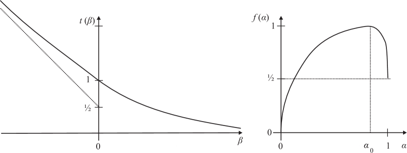
Figure 1.1. The arithmetic-geometric free energy function $t$ and the associated multifractal scaling spectrum $f$.

Theorem 1.8.

The Hausdorff dimension spectrum (cf. Fig. 1.1) for the arithmetic-geometric scaling is given by

$$f\left(\alpha\right)=\max\left\{-\widehat{t}\left(-\alpha\right),0\right\}=\dim_{H}\left(\mathcal{F}_{\alpha}^{*}\right),\qquad\alpha\in\mathbb{R}.$$

The function $f\big{|}_{\left[0,1\right]}$ is strictly convex, continuous, and real-analytic on $\left(0,1\right)$. It attains its maximal value $1$ in $\alpha_{0}=12\pi^{-2}\log\left(2\right)\log\left(K_{0}\right)$, where $K_{0}$ denotes the Khintchin constant. For the boundary points we have

$$f\left(0\right)=0,\>\>f\left(1\right)=1/2,\>\>\mbox{and }\>\lim_{\alpha\searrow 0}f^{\prime}\left(\alpha\right)=+\infty,\>\>\lim_{\alpha\nearrow 1}f^{\prime}\left(\alpha\right)=-\infty.$$

The remaining part of this section is devoted to the significance of the particular value $f\left(1\right)=\dim_{H}\left(\mathcal{F}_{1}\right)=1/2$. We have already noticed that $\mathcal{F}_{1}$ contains the set $\mathcal{G}$ of points $x\in\mathbb{I}$ with continued fraction entries $a_{i}\left(x\right)$ tending to infinity. For this set Good proved in [Goo41] that

(1.4) $$\dim_{H}\mathcal{G}=1/2.$$

Since $\mathcal{F}_{1}\supset\mathcal{G}$, Good’s results provides us with a lower but not with an upper bound for $f\left(1\right)$. In [KS07b] it has been shown, that the Hausdorff dimension of sets with large geometric scaling coefficients are close to $1/2$, i.e.

$$\dim_{H}\left\{x\in\left(0,1\right):\lim_{n\rightarrow\infty}\frac{2\log q_{n}\left(x\right)}{n}=\alpha\right\}\to 1/2,\quad\alpha\to\infty.$$

Similarly, in [FLWW08] we find for $\alpha>1$ and $\beta>0$,

$$\dim_{H}\left\{x\in\left(0,1\right):\lim_{n\rightarrow\infty}\frac{\log q_{n}\left(x\right)}{n^{\alpha}}=\beta\right\}=1/2.$$

Ramharter has shown in [Ram85] that also for every $q\in\mathbb{N}$ we have

$$\dim_{H}\left\{x\in\mathbb{I}:a_{i}\left(x\right)\geq q;a_{i}\left(x\right)\neq a_{j}\left(x\right)\>\mbox{for all }i\neq j\right\}=1/2.$$

Other results interesting in this context can be found in [Ram94], [Cus90], [Hir73] and [Hir70] . Furthermore, in [Ram85] we find that for $q\to\infty$

(1.5) $$\dim_{H}\mathcal{I}_{q}=\frac{1}{2}+\mbox{O}\left(\frac{\log\log q}{\log q}\right),$$

where O denotes the usual Landau symbol, i.e. $f\left(x\right)=\mbox{O}\left(g\left(x\right)\right)$ for $x\to a$ if there exists a constant $c>0$ such that $f\left(x\right)\leq cg\left(x\right)$ for all $x$ in a neighbourhood of $a$. With some extra effort we are able to improve (1.5) and obtain the precise asymptotic of this convergence. Here $a\left(n\right)\sim b\left(n\right)$ stands for $a\left(n\right)/b\left(n\right)\to 1$ for $n\to\infty$.

Proposition 1.9.

For $q\to\infty$ we have

$$\dim_{H}\mathcal{I}_{q}-\frac{1}{2}\sim\frac{1}{2}\frac{\log\log q}{\log q}.$$

We would like to remark that this result is rather complementary to the Texan conjecture (proved in [KZ06]), which claims that the set of Hausdorff dimensions of bounded type continued fraction sets is dense in the unit interval. Already Jarník observed in [Jar29] that for the set of bounded continued fractions we have

$$\dim_{H}\left\{x\in\mathbb{I}:\forall i\in\mathbb{N}\;a_{i}\left(x\right)\leq M\right\}=1-\mbox{O}\left(1/M\right).$$

This was later significantly improved by Hensley, who gave a precise asymptotic up to $\mbox{O}\left(M^{-2}\right)$ in [Hen92].

As an interesting application of our multifractal analysis we are able to give an asymptotic formula for the Hausdorff dimension of $\mathcal{F}_{\alpha}$ as $\alpha$ approaches $1$. Let us write $a\left(x\right)=\Theta(b(x))$ for $x\nearrow a$ if there exist constants $0<c_{1}\leq c_{2}$ such that $c_{1}b\left(x\right)\leq a\left(x\right)\leq c_{2}b\left(x\right)$ for all $x$ in a (left) neighbourhood of $a$.

Theorem 1.10.

For $\alpha\nearrow 1$ we have

$$f(\alpha)=\frac{1}{2}+\Theta\left(\frac{\log\log\left(1/\left(1-\alpha\right)\right)}{\log\left(1/\left(1-\alpha\right)\right)}\right).$$

Remark 1.11.

Actually, the constants in the definition of $\Theta$ can be chosen to be any $0<c_{1}<1$ and $c_{2}>2$.

In virtue of Fact 1.6 there is a connection between Theorem 1.10 and Proposition 1.9, which will be employed in the proof of Theorem 1.10.

We would finally like to remark that the arithmetic-geometric scaling allows an interpretation in terms of the geodesic flow on the modular surface. More precisely, the term $\sum\log a_{i}$ measures the homological windings around the cusp, whereas $\log q_{n}$ stands for the total geodesic length. The set $\mathbb{I}$ is regarded as the set of directions for a given observation point. This connection allows a generalisation of our formalism also to modular forms similar to [KS07a].

2. Thermodynamic Formalism for the Gauss system

2.1. The Gauss system and Diophantine analysis

The process of writing an element of $\mathbb{I}$ in its unique continued fraction expansion can be restated by a hyperbolic dynamical system given by the Gauss map $T$ defined in (1.1). The Gauss map is conjugated to the left shift $\sigma\colon\mathbb{N}^{\mathbb{N}}\to\mathbb{N}^{\mathbb{N}}$, $\left(\sigma\left(\omega\right)\right)_{i}=\omega_{i+1}$ for $\omega\in\mathbb{N}^{\mathbb{N}}$ via $\pi$, i.e. we have the following commutative diagram

The Gauss system allows alternatively a representation as an infinite conformal Iterated Function System as defined in [MU03]. The system is given by the compact metric space $\left[0,1\right]$ together with the inverse branches $\Phi_{n}\colon\left[0,1\right]\to\left[0,1\right]$, $x\mapsto\left(n+x\right)^{-1}$, $n\in\mathbb{N}$, of the Gauss map. Notice that the family of maps $\left(\Phi_{n}\Phi_{m}\right)_{n,m}$ is uniformly contracting. We are now aiming at expressing the arithmetic-geometric scaling limit in dynamical terms. For this we introduce the two potential functions

$$\psi\colon\mathbb{N}^{\mathbb{N}}\to\mathbb{R}_{0}^{-},\>\omega\mapsto-2\log\omega_{1}\;\mbox{ and }\;\varphi\colon\mathbb{N}^{\mathbb{N}}\to\mathbb{R}^{-},\>\omega\mapsto-\log\left(|T^{\prime}\left(\pi^{-1}\left(\omega\right)\right)|\right),$$

where $\psi$ describes the arithmetic properties, while $\varphi$ describes the geometric properties of the continued fraction expansion. We will equip $\mathbb{N}^{\mathbb{N}}$ with the metric $d$ given by $d(\omega,\tau):=\exp\left(-|\omega\wedge\tau|\right),$ where $|\omega\wedge\tau|$ denotes the length of the longest common initial block of $\omega$ and $\tau$. Since $\psi$ is locally constant we immediately see that $\psi$ is Hölder continuous with respect to this metric. Next, we want to show that also $\varphi$ is Hölder continuous. We start with an important observation connecting the arithmetic and geometric properties of the continued fraction expansion. For two sequences $\left(a_{n}\right)$, $\left(b_{n}\right)$ we will write $a_{n}\ll b_{n}$, if $a_{n}\leq Kb_{n}$ for some $K>0$ and all $n\in\mathbb{N}$, and if $a_{n}\ll b_{n}$ and $b_{n}\ll a_{n}$ then we write $a_{n}\asymp b_{n}$. For $\omega\in\mathbb{N}^{\mathbb{N}}$ and $n\in\mathbb{N}$ let $\omega|_{n}:=\left(\omega_{1},\dots,\omega_{n}\right)$ and let $[\omega|_{n}]:=\left\{\tau\in\mathbb{N}^{\mathbb{N}}:\tau_{1}=\omega_{1},\dots,\tau_{n}=\omega_{n}\right\}$ denote the $n$-cylinder of $\omega$. Since we always have $p_{n-1}\left(\omega\right)q_{n}\left(\omega\right)-p_{n}\left(\omega\right)q_{n-1}\left(\omega\right)=\left(-1\right)^{n}$ and

$$\pi^{-1}\left(\left[\omega|_{n}\right]\right):=\begin{cases}\vspace{2pt}\left(\frac{p_{n}\left(\omega\right)}{q_{n}\left(\omega\right)},\frac{p_{n}\left(\omega\right)+p_{n-1}\left(\omega\right)}{q_{n}\left(\omega\right)+q_{n-1}\left(\omega\right)}\right)\cap\mathbb{I}&\mbox{for }n\,\mbox{ even,}\\ \left(\frac{p_{n}\left(\omega\right)+p_{n-1}\left(\omega\right)}{q_{n}\left(\omega\right)+q_{n-1}\left(\omega\right)},\frac{p_{n}\left(\omega\right)}{q_{n}\left(\omega\right)}\right)\cap\mathbb{I}&\mbox{for }n\,\mbox{ odd},\end{cases}$$

it follows that

$$\mathrm{diam}\left(\pi^{-1}[\omega_{|n}]\right)=q_{n}\left(\omega\right)^{-1}\left(q_{n}\left(\omega\right)+q_{n-1}\left(\omega\right)\right)^{-1}=q_{n}\left(\omega\right)^{-2}\left(1+\frac{q_{n-1}\left(\omega\right)}{q_{n}\left(\omega\right)}\right)^{-1}$$

for all $n\in\mathbb{N}$ (see e.g. [Khi56]). This gives

(2.1) $$\mathrm{diam}\left(\pi^{-1}[\omega_{|n}]\right)\asymp\frac{1}{q_{n}^{2}\left(\omega\right)}$$

where the constants are independent of $\omega\in\mathbb{N}^{\mathbb{N}}$. With $f_{n}$ denoting the $n$-th Fibonacci number we have that $q_{n}\left(\omega\right)\geq f_{n}\gg\gamma^{n}$, where $\gamma:=\left(\sqrt{5}+1\right)/2$ refers to the Golden Mean. Fix $v,w\in[\omega]$ for some $\omega\in\mathbb{N}^{n}$. Then, using (2.1), we get

$$\left|\varphi\left(v\right)-\varphi\left(w\right)\right| = 2\left|\log\left(\pi^{-1}v\right)-\log\left(\pi^{-1}w\right)\right|=2\left|\log\left(1+\frac{\pi^{-1}w-\pi^{-1}v}{\pi^{-1}v}\right)\right|$$

$$\ll \frac{q_{n}\left(\omega\right)}{p_{n}\left(\omega\right)}q_{n}\left(\omega\right)^{-2}\ll d\left(v,w\right)^{2\log\gamma},$$

which proves the Hölder continuity of $\varphi$. From this we also deduce the so-called bounded distortion property

(2.2) $$\frac{\left|\varphi_{\omega|_{n}}^{\prime}\left(x\right)\right|}{\left|\varphi_{\omega|_{n}}^{\prime}\left(y\right)\right|}\asymp 1,$$

where $\varphi_{\omega|_{n}}:=\varphi_{\omega_{1}}\circ\cdots\circ\varphi_{\omega_{n}}$ and the constants are independent of $\omega\in\mathbb{N}^{\mathbb{N}}$ and $x,y\in\mathbb{I}$. The bounded distortion property in particular implies $\left|\varphi_{\omega|_{n}}^{\prime}\left(x\right)\right|\asymp\mathrm{diam}\left(\pi^{-1}[\omega|_{n}]\right).$ Using this it is possible to compare the diameters of cylinder sets with orbit sums $S_{n}\varphi:=\sum_{k=0}^{n-1}\varphi\circ\sigma^{k}$ with respect to the geometric potential $\varphi$ under iterations of the shift map $\sigma$ . In fact, by the chain rule and (2.2) we have uniformly for $\omega\in\mathbb{N}^{\mathbb{N}}$ and $\tau\in\left[\omega|_{n}\right]$

(2.3) $$\exp S_{n}\varphi\left(\tau\right)\asymp\mathrm{diam}\left(\pi^{-1}[\omega|_{n}]\right).$$

2.2. Topological pressure

The topological pressure $\mathfrak{P}\left(t\varphi+\beta\psi\right)$ of the potential $t\varphi+\beta\psi$ for $t,\beta\in\mathbb{R}$ is defined as

$$\mathfrak{P}\left(t\varphi+\beta\psi\right):=\lim_{n\rightarrow\infty}\frac{1}{n}\log\sum_{\omega\in\mathbb{N}^{n}}\exp\sup_{\tau\in[\omega]}\left(S_{n}t\varphi+\beta\psi\right)(\tau).$$

By a standard argument involving sub-additivity the above limit always exists.

The next lemma shows, that the set $\mathcal{F}_{\alpha}$ can be characterized by the potentials $\varphi$ and $\psi$ and that the arithmetic-geometric pressure $P$$\left(t,\beta\right)$ agrees with $\mathfrak{P}\left(t\varphi+\beta\psi\right)$, $t,\beta\in\mathbb{R}$.

Lemma 2.1.

For $\alpha\in\mathbb{R}$ and $x\in\mathbb{I}$ we have

$$\lim_{n\rightarrow\infty}\frac{S_{n}\psi\left(\pi\left(x\right)\right)}{S_{n}\varphi\left(\pi\left(x\right)\right)}=\alpha\iff\lim_{n\rightarrow\infty}\frac{\log\prod_{j=1}^{n}a_{j}\left(x\right)}{\log q_{n}\left(x\right)}=\alpha$$

and

$$P\left(t,\beta\right)=\mathfrak{P}\left(t\varphi+\beta\psi\right),\qquad t,\beta\in\mathbb{R}.$$

Proof.

By (2.1) and (2.3) there exist constants $C_{1},C_{2}>0$, such that for all $\omega\in\mathbb{N}^{\mathbb{N}}$ and $n\in\mathbb{N}$ we have

(2.4) $$-2\log q_{n}\left(\omega\right)+\log C_{1}\leq S_{n}\varphi\left(\omega\right)\leq-2\log q_{n}\left(\omega\right)+\log C_{2}.$$

Dividing this inequality by $S_{n}\psi\left(\omega\right)=-2\log\left(\prod_{j=1}^{n}\omega_{j}\right)$ and using the fact that $q_{n}\left(\omega\right)$ tends to infinity for $n\rightarrow\infty$ proves the first assertion.

To prove the second claim notice that by (2.1) and the definition of $\psi$ we have

$$\sum_{\omega\in\mathbb{N}^{n}}\exp\sup_{\tau\in[\omega]}\left(S_{n}t\varphi+\beta\psi\right)(\tau) \asymp \sum_{\omega\in\mathbb{N}^{n}}q_{n}^{-2t}\left(\omega\right)\left(\prod_{j=1}^{n}\omega_{j}\right)^{-2\beta}.$$

Taking logarithms and dividing by $n$ again proves the claim. ∎

Lemma 2.2.

We have

(2.5) $$P\left(t,\beta\right)<\infty\iff 2\left(t+\beta\right)>1.$$

Proof.

Using (1.3) we have on the one hand for $t\leq 0$

$$\zeta\left(2\left(t+\beta\right)\right)^{n}\ll\sum_{\omega\in\mathbb{N}^{n}}q_{n}^{-2t}\left(\omega\right)\left(\prod_{j=1}^{n}\omega_{j}\right)^{-2\beta}\ll 2^{-2nt}\zeta\left(2\left(t+\beta\right)\right)^{n},$$

where $\zeta$ denotes the Riemann zeta function, which is singular in $1$. On the other hand for $t>0$ we have

$$2^{-2nt}\zeta\left(2\left(t+\beta\right)\right)^{n}\ll\sum_{\omega\in\mathbb{N}^{n}}q_{n}^{-2t}\left(\omega\right)\left(\prod_{j=1}^{n}\omega_{j}\right)^{-2\beta}\ll\zeta\left(2\left(t+\beta\right)\right)^{n}.$$

Taking logarithms and dividing by $n$ then gives in both cases the asserted equivalence. ∎

For later use we will need a refined lower estimate for $q_{n}$, which also relies on the recursion formula (1.2) for $q_{n}$.

Lemma 2.3.

For $\omega=\left(\omega_{1},\omega_{2},\dots\right)\in\mathbb{N}^{\mathbb{N}}$ and $n\in\mathbb{N}$ we have

$$\omega_{1}\prod_{i=2}^{n}\omega_{i}\left(1+\frac{1}{\omega_{i}\left(\omega_{i-1}+1\right)}\right)\leq q_{n}\left(\omega\right)$$

Proof.

The proof is by means of induction. For $n=1$ we have $q_{1}\left(\omega\right)=\omega_{1}$. For $n>1$ we have by the recursion formula (1.2) that

(2.6) $$q_{n}\left(\omega\right)=\omega_{n}q_{n-1}\left(\omega\right)\left(1+\frac{q_{n-2}\left(\omega\right)}{\omega_{n}q_{n-1}\left(\omega\right)}\right)$$

and also

(2.7) $$\frac{q_{n-1}\left(\omega\right)}{q_{n-2}\left(\omega\right)}=\omega_{n-1}+\frac{q_{n-3}\left(\omega\right)}{q_{n-2}\left(\omega\right)}\leq\omega_{n-1}+1.$$

Combining (2.7) and (2.6) gives

$$\omega_{n}\left(1+\frac{1}{\omega_{n}\left(\omega_{n-1}+1\right)}\right)q_{n-1}\left(\omega\right)\leq q_{n}\left(\omega\right),$$

which proves the inductive step. ∎

The next proposition gives bounds for the pressure $P\left(t,\beta\right)$, which will be essential for the discussion of the boundary points of the multifractal spectrum.

Proposition 2.4.

We have for $t\geq 0$

$$\log\negmedspace\left(\sum_{k\in\mathbb{N}}\negmedspace(k+1)^{-2t}k^{-2\beta}\right)\leq P\left(t,\beta\right)\leq\frac{1}{2}\log\negmedspace\left(\sum_{\left(k,l\right)\in\mathbb{N}^{2}}\negmedspace\negmedspace\left(kl\right)^{-2\left(t+\beta\right)}\left(1+\frac{1}{k\left(l+1\right)}\right)^{-2t}\right).$$

Proof.

Using the fact that $q_{n}\left(\omega\right)\leq\prod_{k=1}^{n}\left(\omega_{k}+1\right)$ we obtain a a lower bound

$$\sum_{\omega\in\mathbb{N}^{n}}q_{n}\left(\omega\right)^{-2t}\prod_{i=1}^{n}a_{i}^{-2\beta} \geq \sum_{\omega\in\mathbb{N}^{n}}\prod_{i=1}^{n}\left(\omega_{i}+1\right)^{-2t}\omega_{i}^{-2\beta}$$

$$= \left(\sum_{k\in\mathbb{N}}\left(k+1\right)^{-2t}k^{-2\beta}\right)^{n},$$

by rearranging the series. Taking logarithm and dividing by $n$ shows

$$P\left(t,\beta\right)\geq\log\left(\sum_{k\in\mathbb{N}}(k+1)^{-2t}k^{-2\beta}\right).$$

For the upper bound we use Lemma 2.3 to conclude

$$\sum_{\omega\in\mathbb{N}^{k}}q_{k}\left(\omega\right)^{-2t}\prod_{i=1}^{k}\omega_{i}^{-2\beta} \leq \sum_{\omega\in\mathbb{N}^{k}}\left(\omega_{1}\prod_{i=2}^{k}\omega_{i}\left(1+\frac{1}{\omega_{i}\left(\omega_{i-1}+1\right)}\right)\right)^{-2t}\prod_{i=1}^{k}\omega_{i}^{-2\beta}$$

$$= \sum_{\omega\in\mathbb{N}^{k}}\prod_{i=2}^{k}\left(1+\frac{1}{\omega_{i}\left(\omega_{i-1}+1\right)}\right)^{-2t}\prod_{i=1}^{k}\omega_{i}^{-2\left(t+\beta\right)}.$$

Now, we only consider even $k=2n$. Since $\left(1+\left(\omega_{i}\left(\omega_{i-1}+1\right)\right)^{-1}\right)^{-2t}<1$ for all $i\geq 2$, we find an upper bound by omitting all terms with odd indices $i$ in the product $\prod_{i=2}^{2n}\left(1+\left(\omega_{i}\left(\omega_{i-1}+1\right)\right)^{-1}\right)^{-2t}$. Using this and rearranging the series we get

$$\sum_{\omega\in\mathbb{N}^{k}}q_{k}\left(\omega\right)^{-2t}\prod_{i=1}^{k}\omega_{i}^{-2\beta} \leq \sum_{\omega\in\mathbb{N}^{k}}\prod_{i=1}^{n}\left(1+\frac{1}{\omega_{2i}\left(\omega_{2i-1}+1\right)}\right)^{-2t}\left(\omega_{2i-1}\omega_{2i}\right)^{-2\left(t+\beta\right)}.$$

$$= \operatorname*{\sum\cdots\sum}_{\left(\omega_{1},\omega_{2}\right),\left(\omega_{3},\omega_{4}\right),\ldots,\left(\omega_{2n-1},\omega_{2n}\right)\in\mathbb{N}^{2}}\;\prod_{i=1}^{n}\left(1+\frac{1}{\omega_{2i}\left(\omega_{2i-1}+1\right)}\right)^{-2t}\;\left(\omega_{2i-1}\omega_{2i}\right)^{-2\left(t+\beta\right)}\;.$$

$$= \left(\sum_{\left(k,l\right)\in\mathbb{N}^{2}}\left(kl\right)^{-2\left(t+\beta\right)}\left(1+\frac{1}{k\left(l+1\right)}\right)^{-2t}\right)^{\frac{n}{2}}.$$

Taking logarithm and dividing by $n$ gives

$$P\left(t,\beta\right)\leq\frac{1}{2}\log\left(\sum_{\left(k,l\right)\in\mathbb{N}^{2}}\left(kl\right)^{-2\left(t+\beta\right)}\left(1+\frac{1}{k\left(l+1\right)}\right)^{-2t}\right).$$

∎

Remark 2.5.

A straight forward calculation shows that for $t=0$ and $\beta>1/2$ we have

$$P\left(0,\beta\right)=\lim_{n\rightarrow\infty}\frac{1}{n}\log\sum_{\omega\in\mathbb{N}^{n}}\prod_{i=1}^{n}a_{i}\left(\omega\right)^{-2\beta}=\lim_{n\rightarrow\infty}\frac{1}{n}\log\left(\prod_{k=1}^{n}k^{-2\beta}\right)^{n}=\log\left(\zeta\left(2\beta\right)\right).$$

This value coincides for $t=0$ with the upper bound in Proposition 2.4 since

$$\frac{1}{2}\log\left(\sum_{\left(k,l\right)\in\mathbb{N}^{2}}\left(kl\right)^{-2\beta}\right)=\frac{1}{2}\log\left(\sum_{k\in\mathbb{N}}k^{-2\beta}\sum_{l\in\mathbb{N}}l^{-2\beta}\right)=\log\left(\zeta\left(2\beta\right)\right).$$

2.3. Proof of facts

With the results obtain in the previous subsections we are in the position to give the proofs of the Facts 1.1 to 1.7 stated in the introduction.

Proof of Facts 1.1 and 1.2. These facts are immediate consequences of the first inequality in (1.3). ∎

Proof of Fact 1.3. First notice that $\pi^{-1}\left(k,k,\dots\right)$, $k\in\mathbb{N}$, is a fixed point of the Gauss map $T$ and hence invariant under $x\mapsto 1/x-k$. This implies $\pi^{-1}\left(k,k,\dots\right)=-k/2+\sqrt{k^{2}/4+1}$. Using (2.4) in the proof of Lemma 2.1 gives for $q_{n}:=q_{n}\left(\left(k,k,\ldots\right)\right)$

$$\lim_{n\to\infty}\frac{\log q_{n}}{n}=-\frac{1}{2}\varphi\left(\left(k,k,\ldots\right)\right)=-\log\left(\pi^{-1}\left(k,k,\ldots\right)\right)=-\log\left(-k/2+\sqrt{k^{2}/4+1}\right).$$

From this the claims follow. ∎

Proof of Fact 1.4. Using (1.3) we have

$$\frac{\sum_{i=1}^{n}\log a_{i}\left(x\right)}{\log q_{n}\left(x\right)} \geq \frac{\sum_{i=1}^{n}\log a_{i}\left(x\right)}{n\log 2+\sum_{i=1}^{n}\log a_{i}\left(x\right)}$$

$$= \left(\frac{\log 2}{n^{-1}\sum_{i=1}^{n}\log a_{i}\left(x\right)}+1\right)^{-1}\to 1,\qquad n\to\infty.$$

Here we have used that the Cesàro mean of $\log a_{i}\left(x\right)$ tends to infinity. ∎

Proof of Fact 1.5. Let us consider the ergodic dynamical system $\left(\mathbb{I},T,\lambda_{g}\right)$ where $d\lambda_{g}\left(x\right):=\left(\log\left(2\right)\left(1+x\right)\right)^{-1}d\lambda\left(x\right)$ denotes the famous Gauss measure. By the Ergodic Theorem we have $\lambda_{g}$-a.e. and consequently $\lambda$-a.e.

$$\lim_{n}\frac{S_{n}\psi}{n}:=\int\psi\,d\lambda_{g}=\frac{-2}{\log 2}\sum_{k=1}^{\infty}\log\left(k\right)\log\left(1+\frac{1}{k\left(k+2\right)}\right)=-2\log\left(K_{0}\right)$$

as well as

$$\lim_{n}\frac{S_{n}\varphi}{n}:=\int\varphi\,d\lambda_{g}=\frac{2}{\log 2}\int\frac{\log\left(x\right)}{\left(1+x\right)}\,d\lambda=\frac{-\zeta\left(2\right)}{\log 2}=\frac{-\pi^{2}}{6\log 2}.$$

From this the fact follows immediately. ∎

Proof of Fact 1.6. Using the inequality $q_{n}\left(x\right)\leq\prod_{i=1}^{n}\left(a_{i}\left(x\right)+1/q\right)$ for $x\in\mathcal{I}_{q}$ and $n\in\mathbb{N}$ we have

${\displaystyle\frac{\sum_{i=1}^{n}\log a_{i}\left(x\right)}{\log q_{n}\left(x\right)}}$

$$\geq \frac{\sum_{i=1}^{n}\log a_{i}\left(x\right)}{\sum_{i=1}^{n}\log\left(a_{i}\left(x\right)+1/q\right)}=\frac{\sum_{i=1}^{n}\log a_{i}\left(x\right)}{\sum_{i=1}^{n}\log a_{i}\left(x\right)+\sum_{i=1}^{n}\log\left(1+1/qa_{i}\left(x\right)\right)}$$

$$= \frac{\sum_{i=1}^{n}\log a_{i}\left(x\right)}{\sum_{i=1}^{n}\log a_{i}\left(x\right)+\sum_{i=1}^{n}\log\left(1+1/qa_{i}\left(x\right)\right)}\geq\frac{\sum_{i=1}^{n}\log a_{i}\left(x\right)}{\sum_{i=1}^{n}\log a_{i}\left(x\right)+n/q^{2}}$$

$$= \left(1+\frac{n}{q^{2}\sum_{i=1}^{n}\log a_{i}\left(x\right)}\right)^{-1}\geq\left(1+\left(q^{2}\log\left(q\right)\right)^{-1}\right)^{-1}$$

$$= 1-\frac{\left(q^{2}\log\left(q\right)\right)^{-1}}{1+\left(q^{2}\log\left(q\right)\right)^{-1}}\geq 1-\left(q^{2}\log\left(q\right)\right)^{-1}.\hskip 85.35826pt\qed$$

Proof of Fact 1.7. We show that $\mathcal{B}\subset\mathbb{I}\setminus\mathcal{F}_{1}$. Let us assume that for an element $x\in\mathcal{B}$ the sequence $\left(a_{i}\left(x\right)\right)_{i\in\mathbb{N}}$ is bounded by $M\geq 2$. Then using the lower bound for $q_{n}$ provided in Lemma 2.3 and the fact that $\log\left(1+t\right)\geq t\cdot\log(2),$ $t\in\left[0,1\right]$ we calculate for $n\geq 2$

$$\frac{\sum_{i=1}^{n}\log a_{i}\left(x\right)}{\log q_{n}\left(x\right)} \leq \frac{\sum_{i=1}^{n}\log a_{i}\left(x\right)}{\sum_{i=1}^{n}\log a_{i}\left(x\right)+\sum_{i=2}^{n}\log\left(1+\left(a_{i}\left(x\right)\left(a_{i-1}\left(x\right)+1\right)\right)^{-1}\right)}$$

$$\leq \left(1+\frac{\sum_{i=2}^{n}\log\left(2\right)/a_{i}\left(x\right)\left(a_{i-1}\left(x\right)+1\right)}{\sum_{i=1}^{n}\log a_{i}\left(x\right)}\right)^{-1}$$

$$\leq \left(1+\frac{\log 2\left(n-1\right)}{M\left(M+1\right)n\log M}\right)^{-1}$$

$$\leq \left(1+\frac{\log 2}{2M\left(M+1\right)\log M}\right)^{-1}<1.$$

Since the left hand side is bounded away from $1$ by a constant only depending on $M$ the fact follows. ∎

2.4. Gibbs states

Let us recall some basic facts about Gibbs states taken from [MU03]. For a continuous function $f\colon\mathbb{N}^{\mathbb{N}}\to\mathbb{R}$ a Borel probability measure $m$ on $\mathbb{N}^{\mathbb{N}}$ is called a Gibbs state for $f$, if there exists a constant $Q\geq 1$ such that for every $n\in\mathbb{N}$, $\omega\in\mathbb{N}^{n}$ and $\tau\in[\omega]$ we have

(2.8) $$Q^{-1}\leq\frac{m([\omega])}{\exp(S_{n}f(\tau)-n\mathfrak{P}\left(f\right))}\leq Q.$$

If in addition the measure $m$ is $\sigma$-invariant then $m$ is called an invariant Gibbs state for $f$.

Also the concept of the metric entropy will by crucial. Recall that in our situation for a $\sigma$-invariant measure $\mu$ the metric entropy is given by

$$h_{\mu}:=\lim_{n}\frac{1}{n}\sum_{\omega\in\mathbb{N}^{n}}\mu\left(\left[\omega\right]\right)\log\left(\mu\left(\left[\omega\right]\right)\right),$$

where as usual we set $0\cdot\log 0=0$. Note, that the above limit always exists (see e.g. [Wal82]).

The next proposition states the key result of the Thermodynamic Formalism in our context, that is the existence and uniqueness of equilibrium measures for the Hölder continuous and summable potential $t\varphi+\beta\psi$ with $2\left(t+\beta\right)>1$, i.e. $\sum_{k\in\mathbb{N}}\exp\sup_{\tau\in\left[k\right]}\left(t\varphi+\beta\psi\right)\left(\tau\right)<\infty$. For a proof we refer to [MU03] (see e.g. [Bow75] for a classical version valid for compact state spaces).

Proposition 2.6.

For each  $\left(t,\beta\right)\in\mathbb{R}^{2}$ such that  $2\left(t+\beta\right)>1$ there exists a unique invariant Gibbs state $\mu_{t\varphi+\beta\psi}$ for the potential $t\varphi+\beta\psi$, which is ergodic and an equilibrium state for the potential, i.e. $P\left(t,\beta\right)=h_{\mu_{t\varphi+\beta\psi}}+\int t\varphi+\beta\psi\,d\mu_{t\varphi+\beta\psi}$.

We close this subsection with a technical lemma needed for the proof of Proposition 2.9.

Lemma 2.7.

For each $\left(t,\beta\right)\in\mathbb{R}^{2}$ such that $2\left(t+\beta\right)>1$ we have $\varphi,\psi\in\mathcal{L}\left(\mu_{t\varphi+\beta\psi}\right)$.

Proof.

Since we have $|\psi|\leq|\varphi|$ it suffices to show $\varphi\in\mathcal{L}\left(\mu_{t\varphi+\beta\psi}\right)$. We have

$$\int|\varphi|\,d\mu_{t\varphi+\beta\psi} \leq \sum_{i\in\mathbb{N}}\sup\left(|\varphi|_{|\left[i\right]}\right)\mu_{t\varphi+\beta\psi}\left(\left[i\right]\right).$$

Observing $\sup\left(|\varphi|_{|\left[i\right]}\right)\leq\log\left(i+1\right)$ and using the Gibbs property (2.8) for $\mu_{t\varphi+\beta\psi}$ we have

$$\sum_{i\in\mathbb{N}}\sup\left(|\varphi|_{|\left[i\right]}\right)\mu_{t\varphi+\beta\psi}\left(\left[i\right]\right) \ll \sum_{i\in\mathbb{N}}\log\left(i+1\right)\exp\sup\left(t\varphi+\beta\psi_{|\left[i\right]}\right)$$

$$\ll \sum_{i\in\mathbb{N}}\log\left(i+1\right)\frac{1}{i^{2\left(t+\beta\right)}}<\infty.$$

∎

2.5. The arithmetic-geometric free energy

To guarantee that the free energy function is non-linear and hence the multifractal spectrum is non-trivial we need the following observation.

Lemma 2.8.

The potentials $\varphi$ and $\psi$ are linear independent in the cohomology class of bounded Hölder continuous functions, i.e. for every bounded Hölder continuous function $u$ satisfying $\alpha\varphi+\beta\psi=u-u\circ\sigma$ we have $\alpha=\beta=0$.

Proof.

Suppose there exists a bounded Hölder continuous function $u:\mathbb{N}^{\mathbb{N}}\to\mathbb{R}$, such that

$$\alpha\varphi+\beta\psi=u-u\circ\sigma.$$

Since $u$ is bounded, there exists $C<\infty$, such that for all $n\in\mathbb{N}$

$$\left\|S_{n}\left(u-u\circ\sigma\right)\right\|=\left\|u-u\circ\sigma^{n}\right\|<C$$

where $\left\|\cdot\right\|$ denotes the uniform norm on the space of bounded continuous functions. This implies for all $n\in\mathbb{N}$

(2.9) $$\left\|\alpha S_{n}\varphi+\beta S_{n}\psi\right\|<C.$$

For $\omega=\left(1,1,1,\dots\right)$ we have $\beta S_{n}\psi(\omega)+\alpha S_{n}\varphi\left(\omega\right)=\alpha S_{n}\varphi\left(\omega\right)=2n\alpha\log\gamma$ for all $n\in\mathbb{N}$. This stays bounded only for $\alpha=0$. Furthermore, for $\omega=\left(2,2,2,\ldots\right)$ we have $\beta S_{n}\psi=2n\beta\log(2)$ for all $n\in\mathbb{N}$. Again this stays bounded only if also $\beta=0$. ∎

Proposition 2.9.

For each $\beta\in\mathbb{R}$ there exists a unique number $t\left(\beta\right)$ such that

(2.10) $$P\left(t\left(\beta\right),\beta\right)=0.$$

The arithmetic-geometric free energy function $t$ defined in this way is real-analytic and strictly convex, and we have

(2.11) $$t^{\prime}\left(\beta\right)=-\frac{\int\psi\,d\mu_{\beta}}{\int\varphi\,d\mu_{\beta}}<0,$$

where $\mu_{\beta}$ denotes the unique invariant Gibbs state for $t\left(\beta\right)\varphi+\beta\psi$.

Proof.

By [MU03, Theorem 2.6.12] we know that the pressure $P$ is real-analytic on $\left\{\left(t,\beta\right)\in\mathbb{R}^{2}:P\left(t,\beta\right)<\infty\right\}$. Hence by Lemma 2.2, $P$ is real-analytic precisely on$\left\{2\left(t+\beta\right)>1\right\}$. By [MU03, Proposition 2.6.13] the partial derivatives can be expressed as integrals, i.e.

$$\frac{\partial}{\partial\beta}P\left(t,\beta\right)=\int\psi\,d\mu_{t\varphi+\beta\psi},\;\frac{\partial}{\partial t}P\left(t,\beta\right)=\int\varphi\,d\mu_{t\varphi+\beta\psi},$$

where Lemma 2.7 assures that $\varphi,\psi\in\mathcal{L}\left(\mu_{t\varphi+\beta\psi}\right)$ for all $\left(t,\beta\right)$ with $2\left(t+\beta\right)>1$. Since $\mu$ is ergodic we have

$$\int\varphi\,d\mu\leq\sup_{x\in\mathbb{N}^{\mathbb{N}}}\limsup_{n}\frac{S_{n}\varphi\left(x\right)}{n}=\varphi\left(\left(1,1,1,\ldots\right)\right)=-2\log\gamma,$$

where again $\gamma$ denotes the Golden Mean. Consequently,

(2.12) $$\frac{\partial}{\partial t}P\left(t,\beta\right)=\int\varphi\,d\mu_{t\varphi+\beta\psi}\leq-2\log\gamma<0$$

is bounded away from zero.

Now let $\beta\in\mathbb{R}$. By Lemma 2.2 we have that $P\left(t,\beta\right)<\infty$, if and only if $2\left(t+\beta\right)>1$. Also, since $\lim_{t\searrow\frac{1}{2}-\beta}P\left(t,\beta\right)=\infty$ we find $t_{0}\in\mathbb{R}$ such that $0<P\left(t_{0},\beta\right)<\infty$. By (2.12) we conclude that there exists a unique $t=t\left(\beta\right)$ with $P\left(t\left(\beta\right),\beta\right)=0$. By the implicit function theorem and (2.12) we have that the function $t$ is real-analytic and

(2.13) $$t^{\prime}\left(\beta\right)=-\frac{\frac{\partial}{\partial\beta}P\left(t\left(\beta\right),\beta\right)}{\frac{\partial}{\partial t}P\left(t\left(\beta\right),\beta\right)}=-\frac{\int\psi\,d\mu_{\beta}}{\int\varphi\,d\mu_{\beta}}<0.$$

Concerning the strict convexity of $t$ we follow [KS07a]. Observe that

$$-\frac{\partial}{\partial t}P\left(t\left(\beta\right),\beta\right)t^{\prime\prime}\left(\beta\right)=\sigma_{\beta}^{2}\left(t^{\prime}\left(\beta\right)\varphi+\psi\right)\geq 0,$$

where

$\sigma_{\beta}^{2}\left(t^{\prime}\left(\beta\right)\varphi+\psi\right)=$

$$\lim_{n\longrightarrow\infty}\frac{1}{n}\int\left(S_{n}\left(\left(t^{\prime}\left(\beta\right)\varphi+\psi\right)-\int\left(t^{\prime}\left(\beta\right)\varphi+\psi\right)\,d\mu_{\beta}\right)\right)^{2}\,d\mu_{\beta}$$

is the asymptotic variance of $S_{n}\left(t^{\prime}\left(\beta\right)\varphi+\psi\right)$ with respect to the invariant Gibbs measure $\mu_{\beta}$. Since $\int\left(t^{\prime}\left(\beta\right)\varphi+\psi\right)\,d\mu_{\beta}=0$ by (2.13) we can conclude by ([MU03, Lemma 4.88]) that $\sigma_{\beta}^{2}\left(t^{\prime}\left(\beta\right)\varphi+\psi\right)>0$, since $\varphi$ and $\psi$ are elements of $\mathcal{L}^{2}\left(\mu_{\beta}\right)$ by Lemma 2.7 and are linearly independent in the cohomology class of bounded Hölder continuous functions by Lemma 2.8. ∎

The following lemma will be crucial for the the asymptotic properties of $f$ in $1$ and will be used in the proofs of the main theorems in Section 3.

Lemma 2.10.

For all $0<\epsilon<1/2$ we have

$$t\left(\beta\left(\epsilon\right)\right)<1/2-\beta\left(\epsilon\right)+\frac{\epsilon}{2}\quad\mbox{with }\;\beta\left(\epsilon\right):=\frac{3}{\log(2)}\log\left(\epsilon\right)\left(\frac{\epsilon}{3}\right)^{-4/\epsilon}.$$

Proof.

Let us assume on the contrary that there exists $0<\epsilon<1/2$ such that $t\left(\beta\left(\epsilon\right)\right)\geq 1/2-\beta\left(\epsilon\right)+\epsilon/2$. This implies $-2\left(t\left(\beta\left(\epsilon\right)\right)+\beta\left(\epsilon\right)\right)\leq-\left(1+\epsilon\right)$ as well as $-2t\left(\beta\left(\epsilon\right)\right)\leq 2\beta\left(\epsilon\right)-\epsilon-1\leq 2\beta\left(\epsilon\right)$. Consequently, by definition of $t$ and Proposition 2.4 we would have

$$0 = P\left(t\left(\beta\left(\epsilon\right)\right),\beta\left(\epsilon\right)\right)$$

$$\leq \frac{1}{2}\log\sum_{\left(k,l\right)\in\mathbb{N}^{2}}\left(kl\right)^{-2\left(t\left(\beta\left(\epsilon\right)\right)+\beta\left(\epsilon\right)\right)}\left(1+\frac{1}{k\left(l+1\right)}\right)^{-2t\left(\beta\left(\epsilon\right)\right)}$$

$$\leq \frac{1}{2}\log\sum_{\left(k,l\right)\in\mathbb{N}^{2}}\left(kl\right)^{-\left(1+\epsilon\right)}\left(1+\frac{1}{k\left(l+1\right)}\right)^{2\beta\left(\epsilon\right)}.$$

To obtain a contradiction we will show that

$$\sum_{\left(k,l\right)\in\mathbb{N}^{2}}\left(kl\right)^{-\left(1+\epsilon\right)}\left(1+\frac{1}{k\left(l+1\right)}\right)^{2\beta\left(\epsilon\right)}<1.$$

In fact, for $N\left(\epsilon\right):=\left(\epsilon/3\right)^{-2/\epsilon}$ we have for $0<\epsilon<1/2$ that

• ${\displaystyle{\displaystyle\operatorname*{\sum\sum}_{k>N\left(\epsilon\right)\textrm{ or }l>N\left(\epsilon\right)}\left(kl\right)^{-\left(1+\epsilon\right)}\left(1+\frac{1}{k\left(l+1\right)}\right)^{2\beta\left(\epsilon\right)}}<1/2}$      and

• ${\displaystyle\operatorname*{\sum\sum}_{k\leq N\left(\epsilon\right)\textrm{ and }l\leq N\left(\epsilon\right)}\left(kl\right)^{-\left(1+\epsilon\right)}\left(1+\frac{1}{k\left(l+1\right)}\right)^{2\beta\left(\epsilon\right)}}<1/2$.

To prove (A) notice that

${\displaystyle\operatorname*{\sum\sum}_{k>N\left(\epsilon\right)\textrm{ or }l>N\left(\epsilon\right)}\left(kl\right)^{-\left(1+\epsilon\right)}\left(1+\frac{1}{k\left(l+1\right)}\right)^{2\beta\left(\epsilon\right)}}$

$$\leq \sum_{k>N\left(\epsilon\right)}\sum_{l\in\mathbb{N}}\left(kl\right)^{-\left(1+\epsilon\right)}+\sum_{l>N\left(\epsilon\right)}\sum_{k\in\mathbb{N}}\left(kl\right)^{-\left(1+\epsilon\right)}$$

$$\leq 2\sum_{k>N\left(\epsilon\right)}k^{-\left(1+\epsilon\right)}\sum_{l\in\mathbb{N}}l^{-\left(1+\epsilon\right)}$$

Then we have by integral comparison test for $M\in\mathbb{N}$

(2.14) $$\sum_{k>M}k^{-\left(1+\epsilon\right)}\leq\int_{M}^{\infty}x^{-\left(1+\epsilon\right)}dx=\frac{1}{\epsilon}M^{-\epsilon},$$

Hence, for $0<\epsilon<1$,

$$\sum_{k>N\left(\epsilon\right)}k^{-\left(1+\epsilon\right)}\sum_{l\in\mathbb{N}}l^{-\left(1+\epsilon\right)}\leq\frac{1}{\epsilon}N\left(\epsilon\right)^{-\epsilon}\left(\frac{1}{\epsilon}+1\right)\leq\frac{2}{\epsilon^{2}}N\left(\epsilon\right)^{-\epsilon}.$$

With $N\left(\epsilon\right)=\left(\epsilon/3\right)^{-2/\epsilon}$ we get (A).

To verify (B) we use again (2.14) for $0<\epsilon<1$ to obtain

${\displaystyle\operatorname*{\sum\sum}_{k\leq N\left(\epsilon\right)\textrm{ and }l\leq N\left(\epsilon\right)}\left(kl\right)^{-\left(1+\epsilon\right)}\left(1+\frac{1}{k\left(l+1\right)}\right)^{2\beta\left(\epsilon\right)}}$

$$\leq \left(1+\frac{1}{N\left(\epsilon\right)\left(N\left(\epsilon\right)+1\right)}\right)^{2\beta\left(\epsilon\right)}\negmedspace\negmedspace\sum_{k\leq N\left(\epsilon\right)}\sum_{l\leq N\left(\epsilon\right)}\left(kl\right)^{-\left(1+\epsilon\right)}$$

$$\leq \left(1+\frac{1}{2N\left(\epsilon\right)^{2}}\right)^{2\beta\left(\epsilon\right)}\frac{1}{\epsilon^{2}}.$$

We are left to show that

(2.15) $$\left(1+\frac{1}{2N\left(\epsilon\right)^{2}}\right)^{2\beta\left(\epsilon\right)}\frac{1}{\epsilon^{2}}\leq\frac{1}{2},$$

for $0<\epsilon<1/2$. Combining $N\left(\epsilon\right)=\left(\epsilon/3\right)^{-2/\epsilon}$ and $\beta\left(\epsilon\right)=(3/\log 2)\cdot\log\left(\epsilon\right)\cdot\left(\epsilon/3\right)^{-4/\epsilon}$ gives $\beta\left(\epsilon\right)/N\left(\epsilon\right)^{2}=(3/\log 2)\cdot\log\left(\epsilon\right)$. Using this and the fact that $\log\left(1+x\right)\geq x\cdot\log(2),$ $x\in\left[0,1\right]$, we get

$$\log\left(\left(1+\frac{1}{2N\left(\epsilon\right)^{2}}\right)^{2\beta\left(\epsilon\right)}\frac{1}{\epsilon^{2}}\right) \leq 2\beta\left(\epsilon\right)\log\left(1+\frac{1}{2N\left(\epsilon\right)^{2}}\right)-2\log\left(\epsilon\right),$$

$$\leq \log\left(2\right)\frac{\beta\left(\epsilon\right)}{N\left(\epsilon\right)^{2}}-2\log\left(\epsilon\right)$$

$$= \log\left(\epsilon\right)<\log\left(1/2\right)$$

for $0<\epsilon<1/2$. This proves (2.15) and finishes the proof of the lemma. ∎

3. Multifractal Analysis

In this section we prove our main theorems. In the first subsection we prove the upper bound and in the second the lower bound for $f\left(\alpha\right)$. For the upper bound we use a covering argument involving the $n$-th partition function

$$Z_{n}\left(t,\beta\right):=\sum_{\omega\in\mathbb{N}^{n}}\exp\sup_{\tau\in[\omega]}\left(S_{n}t\varphi+\beta\psi\right)(\tau)$$

which is also used to define the topological pressure $P\left(t,\beta\right)$. To prove the lower bound we use the Thermodynamic Formalism to find a measure $\mu$ such that on the one hand $\int\psi\,d\mu/\int\varphi\,d\mu=\alpha$ and on the other hand $\mu$ maximises the quotient of the metrical entropy $h_{\mu}$ and the Lyapunov exponent $\int\varphi\,d\mu$. It will turn out that this measure is in fact the equilibrium measure for the potential $t\left(\beta\right)\varphi+\beta\psi$.

In the last subsection we prove Proposition 1.9 and analyse the boundary points of the spectrum. This part makes extensive use of some number theoretical estimates depending heavily on the recursive nature of the Diophantine approximation.

3.1. Upper bound

For the upper bound we apply a covering argument to the set $\mathcal{F}_{\alpha}^{*}$.

Proposition 3.1.

For $\alpha\in\mathbb{R}$ we have

$$\dim_{H}\left(\mathcal{F}_{\alpha}\right)\leq\dim_{H}\left(\mathcal{F}_{\alpha}^{*}\right)\leq\max\left\{\inf_{\beta\in\mathbb{R}}\left\{t(\beta)+\beta\alpha\right\},0\right\}.$$

If there exists $\beta\in\mathbb{R}$, such that $t\left(\beta\right)+\beta\alpha<0$ then we have $\mathcal{F}_{\alpha}^{*}=\emptyset$.

Proof.

The first inequality follows from $\mathcal{F}_{\alpha}\subset\mathcal{F}_{\alpha}^{*}$. For the second we make the following assumption. For all $\beta\in\mathbb{R}$ and $\epsilon>0$ we have $\mathcal{H}^{t(\beta)+\beta\alpha+\epsilon}\left(\mathcal{F}_{\alpha}^{*}\right)<\infty$, where $\mathcal{H}^{s}$ denotes the $s$-dimensional Hausdorff measure (see [Fal03] for this and related notions from fractal geometry). If then $t(\beta)+\beta\alpha\geq 0$ we can conclude, that $\dim_{H}\left(\mathcal{F}_{\alpha}^{*}\right)\leq t(\beta)+\beta\alpha$. If on the other hand there exists $\beta\in\mathbb{R}$ such that $t\left(\beta\right)+\beta\alpha<0,$ then we would have $\mathcal{H}^{s}\left(\mathcal{F}_{\alpha}^{*}\right)<\infty$ for some $s<0$. This clearly gives $\mathcal{F}_{\alpha}^{*}=\emptyset$ and consequently $\dim_{H}\left(\mathcal{F}_{\alpha}^{*}\right)=0$.

Now we are left to prove the assumption. We will only consider the case $\alpha\geq\alpha_{0}$ (the case $\alpha<\alpha_{0}$ can be treated in a completely analogous way). Then with out loss of generality we may assume that $\beta\leq 0$ (otherwise $t(\beta)+\beta\alpha\geq 1$) . For $r,\delta>0$ fixed we are going to construct a $\delta$-covering of $\pi\left(\mathcal{F}_{\alpha}^{*}\right)$. Since the Gauss system is uniformly contractive, for each $\omega\in\pi\left(\mathcal{F}_{\alpha}^{*}\right)$ there exists $n(\omega,\delta,r)$ such that

(3.1) $$\frac{S_{n(\omega,\delta,r)}\psi\left(\omega\right)}{S_{n(\omega,\delta,r)}\varphi\left(\omega\right)}\geq\alpha-r$$

and

(3.2) $$\mathrm{diam}\left(\pi^{-1}[\omega_{|n(\omega,\delta,r)}]\right)<\delta.$$

We surely have $\pi\left(\mathcal{F}_{\alpha}^{*}\right)\subset\bigcup_{\omega\in\pi\left(\mathcal{F}_{\alpha}\right)}\omega_{|n(\omega,\delta,r)}$. Removing duplicates from the cover, we obtain an at most countable $\delta$-cover $\omega_{|n(\omega^{(i)},\delta,r)}^{(i)}$ with $i\in\mathbb{N}$, because there are only countably many finite words over a countable alphabet.

We will now prove $\mathcal{H}^{t(\beta)+\beta\alpha+\epsilon}\left(\mathcal{F}_{\alpha}^{*}\right)<\infty$ for fixed $\epsilon>0$. Using the cover constructed above we have by the bounded distortion property (2.3) that there exists a constant $C>0$ such that

$$\mathcal{H}_{\delta}^{t(\beta)+\beta\alpha+\epsilon}\left(\mathcal{F}_{\alpha}^{*}\right) \leq \sum_{i\in\mathbb{N}}\mathrm{diam}\left(U_{i}(\delta,r)\right)^{t(\beta)+\beta\alpha+\epsilon}$$

$$= \sum_{i\in\mathbb{N}}\mathrm{diam}\left(\pi^{-1}[\omega_{|n(\omega^{(i)},\delta,r)}^{(i)}]\right)^{t(\beta)+\beta\alpha+\epsilon}$$

$$\leq C\sum_{i\in\mathbb{N}}\exp\left[S_{n(\omega^{(i)},\delta,r)}\varphi(\omega^{(i)})\left(t(\beta)+\beta\alpha+\epsilon\right)\right].$$

Now choose $r>0$ so small, such that for all $i\in\mathbb{N}$ we have

$$\beta\alpha+\epsilon/2>\beta\frac{S_{n(\omega^{(i)},\delta,r)}\psi(\omega^{(i)})}{S_{n(\omega^{(i)},\delta,r)}\varphi(\omega^{(i)})}.$$

Since $S_{n}\varphi<0$ we have

$\mathcal{H}_{\delta}^{t(\beta)+\beta\alpha+\epsilon}\left(\mathcal{F}_{\alpha}^{*}\right)$

$$\leq C\sum_{i\in\mathbb{N}}\exp\left[S_{n(\omega^{(i)},\delta,r)}\varphi(\omega^{(i)})\left(t(\beta)+\beta\frac{S_{n(\omega^{(i)},\delta,r)}\psi(\omega^{(i)})}{S_{n(\omega^{(i)},\delta,r)}\varphi(\omega^{(i)})}+\frac{\epsilon}{2}\right)\right]$$

$$= C\sum_{i\in\mathbb{N}}\exp\left[S_{n(\omega^{(i)},\delta,r)}\varphi(\omega^{(i)})\left(t(\beta)+\frac{\epsilon}{2}\right)+\beta S_{n(\omega^{(i)},\delta,r)}\psi(\omega^{(i)})\right]$$

$$= C\sum_{i\in\mathbb{N}}\exp\left[S_{n(\omega^{(i)},\delta,r)}\left(\left(t(\beta)+\frac{\epsilon}{2}\right)\varphi+\beta\psi\right)(\omega^{(i)})\right]$$

$$\leq C\sum_{n\in\mathbb{N}}\sum_{\omega\in\Sigma^{n}}\exp\sup_{\tau\in[\omega]}\left[S_{n}\left(\left(t(\beta)+\frac{\epsilon}{2}\right)\varphi+\beta\psi\right)\right].$$

Since we have $P\left(t(\beta),\beta\right)=0$ by definition of $t\left(\beta\right)$ and the fact that the pressure $P$ is strictly decreasing with respect to the first component (see (2.12) in the proof of Proposition 2.9), we conclude that $P\left(t(\beta)+\epsilon/2,\beta\right)=\eta<0$. This implies

$$\sum_{\omega\in\Sigma^{n}}\exp\sup_{\tau\in[\omega]}\left(S_{n}\left(\left(t(\beta)+\frac{\epsilon}{2}\right)\varphi+\beta S_{n}\psi\right)\right)\ll\exp\left(n\frac{\eta}{2}\right).$$

Hence, there exists another positive constant $C^{\prime}$ such that for all $\delta>0$ we have $\mathcal{H}_{\delta}^{t(\beta)+\beta\alpha+\epsilon}\left(\mathcal{F}_{\alpha}^{*}\right)\leq C^{\prime}\sum_{n\in\mathbb{N}}\exp\left(n\eta/2\right)<\infty$. This implies $\mathcal{H}^{t(\beta)+\beta\alpha+\epsilon}\left(\mathcal{F}_{\alpha}^{*}\right)<\infty$ showing that $\dim_{H}\left(\mathcal{F}_{\alpha}^{*}\right)\leq t(\beta)+\beta\alpha+\epsilon$ . The claim follows by letting $\epsilon$ tend to zero. ∎

3.2. Lower bound

For the lower bound we use the Volume Lemma ([MU03, Theorem 4.4.2]), which in our situation can be stated as follows. Let $\mu$ be a $\sigma$-invariant probability on $\mathbb{N}^{\mathbb{N}}$ such that either $\sum_{k\in\mathbb{N}}\mu\left(\left[k\right]\right)\log\left(\mu\left(\left[k\right]\right)\right)<\infty$ or $\int\varphi\,d\mu<\infty$. Then

(3.3) $$\mathrm{HD}\left(\mu\right)=\frac{h_{\mu}}{\int\varphi\,d\mu},$$

where $\mathrm{HD}\left(\mu\right):=\inf\left\{\dim_{H}\left(Y\right):Y\subset\mathbb{I},\,\mbox{measurable, }\mu(Y)=1\right\}$. In the following $\mathrm{Im}\left(g\right)$ will denote the image of the function $g$.

Proposition 3.2.

For $\alpha\in-\mathrm{Im}(t^{\prime})$ we have

$$\dim_{H}\left(\mathcal{F}_{\alpha}^{*}\right)\geq\dim_{H}\left(\mathcal{F}_{\alpha}\right)\geq\inf_{\beta\in\mathbb{R}}\left\{t(\beta)+\beta\alpha\right\}>0.$$

Proof.

Again, as for the upper bound, the first inequality is immediate. For $\alpha\in-\mathrm{Im}(t^{\prime})$ let $\beta=\left(t^{\prime}\right)^{-1}\left(-\alpha\right)$. Since $\varphi\in\mathcal{L}^{1}\left(\mu_{t\left(\beta\right)\varphi+\beta\psi}\right)$ we have by the Volume Lemma, Proposition 2.6, the fact that $P\left(t\left(\beta\right),\beta\right)=0$, and (2.11) that

$$\mathrm{HD}\left(\mu_{\beta}\right) = \frac{h_{\mu_{\beta}}}{\int\varphi\,d\mu_{\beta}}=\frac{\int t\left(\beta\right)\varphi+\beta\psi\,d\mu_{\beta}}{\int\varphi\,d\mu_{\beta}}$$

$$= t\left(\beta\right)-\beta t^{\prime}\left(\beta\right)$$

$$= t\left(\left(t^{\prime}\right)^{-1}\left(-\alpha\right)\right)+\left(t^{\prime}\right)^{-1}\left(-\alpha\right)\alpha$$

$$= -\widehat{t}\left(-\alpha\right),$$

where the last equality holds by [Roc70, Theorem 26.4]. By (3.3) we have $-\widehat{t}\left(-\alpha\right)\geq 0$. Furthermore, since $t$ is strictly convex (Proposition 2.9) we conclude with [Roc70, Corollary 26.4.1] that also the Legendre conjugate $\widehat{t}$ is strictly convex on $\mathrm{Im}(t^{\prime})$. Hence, for $\alpha\in-\mathrm{Im}(t^{\prime})$ we have

(3.4) $$\mathrm{HD}\left(\mu_{\beta}\right)=\inf_{c\in\mathbb{R}}\left\{t(c)+c\alpha\right\}>0.$$

Since $\mu_{\beta}$ is ergodic (Proposition 2.6) we have by the Ergodic Theorem, the choice of $\beta$ and (2.11) that

$$\lim_{n\rightarrow\infty}\frac{S_{n}\psi\left(\omega\right)}{S_{n}\varphi\left(\omega\right)}=\frac{\int\psi\,d\mu_{\beta}}{\int\varphi\,d\mu_{\beta}}=\alpha\quad\quad\mbox{for }\mu_{\beta}\mbox{-a.e.}\;\omega.$$

This gives $\mu_{\beta}\left(\mathcal{F}_{\alpha}\right)=1$, which together with (3.4) and the definition of $\mathrm{HD}\left(\mu_{\beta}\right)$ finishes the proof. ∎

Now we can prove the main theorem neglecting the boundary points.

Proof of first part of Theorem 1.8. Clearly, $\mathcal{F_{\alpha}}\subset\mathcal{F}_{\alpha}^{*}$. Combining Proposition 3.1 and Proposition 3.2 gives $f\left(\alpha\right)=\inf_{\beta\in\mathbb{R}}\left\{t(\beta)+\beta\alpha\right\}$ for $\alpha\in-\mathrm{Im}\left(t^{\prime}\right)$. Since also by Proposition 3.2 $f\left(\alpha\right)>0$ for $\alpha\in-\mathrm{Im}\left(t^{\prime}\right)$ we conclude that $-\mathrm{Im}\left(t^{\prime}\right)$ (which is an open set) is contained in $\left(0,1\right)$. Furthermore, for $\alpha\notin-\overline{\mathrm{Im}\left(t^{\prime}\right)}$, we have $\inf_{\beta\in\mathbb{R}}\left\{t(\beta)+\beta\alpha\right\}=-\infty$ ([Roc70, Corollary 26.4.1]), hence by Proposition 3.1 we have $\mathcal{F}_{\alpha}=\emptyset$. Since $\mathcal{F}_{0}$ and $\mathcal{F}_{1}$ are not empty, we have $-\mathrm{Im}\left(t^{\prime}\right)=\left(0,1\right)$. Notice that $f\left(\alpha\right)=-\widehat{t}\left(-\alpha\right)$ for $\alpha\in\left(0,1\right)$ and by [Roc70, Theorem 26.5]

(3.5) $$f^{\prime}\left(\alpha\right)=\left(\widehat{t}\right)^{\prime}\left(-\alpha\right)=\left(t^{\prime}\right)^{-1}\left(-\alpha\right).$$

Since $t^{\prime}$ is strictly increasing we conclude, that $f$ is strictly concave and by the inverse function theorem that $f$ is real-analytic. ∎

3.3. Boundary points

In the last section we finish the proof of Theorem 1.8 and give a proof of Proposition 1.9 and Theorem 1.10.

Proof of the remaining parts of Theorem 1.8. We have to show

• $\lim_{\alpha\searrow 0}f^{\prime}\left(\alpha\right)=\infty$ and $\lim_{\alpha\nearrow 1}f^{\prime}\left(\alpha\right)=-\infty$,

• $\lim_{\alpha\searrow 0}\dim_{H}\left(\mathcal{F}_{\alpha}\right)=\dim_{H}\left(\mathcal{F}_{0}\right)=0$,

• $\lim_{\alpha\nearrow 1}\dim_{H}\left(\mathcal{F}_{\alpha}\right)=\dim_{H}\left(\mathcal{F}_{1}\right)=1/2.$

The assertion in (a) follows directly from equation (3.5). To prove (b) notice that by (2.12) and the definition of $t$ we have for $\beta\in\mathbb{R}$

$$0=P\left(t\left(\beta\right),\beta\right)\leq-2t\left(\beta\right)\log\left(\gamma\right)+P\left(0,\beta\right)$$

which implies $t\left(\beta\right)\leq\frac{P\left(0,\beta\right)}{2\log\left(\gamma\right)}$. Since $P\left(0,\beta\right)=\log\left(\zeta\left(2\beta\right)\right)$, which tends to zero for $\beta\rightarrow\infty$, we conclude that $\lim_{\beta\rightarrow\infty}$$t\left(\beta\right)=0$. By the upper bound in Proposition 3.1, we have that $\dim_{H}\left(\mathcal{F}_{\alpha}\right)$ is dominated by $\inf_{\beta\in\mathbb{R}}\left\{t\left(\beta\right)+\beta\alpha\right\}$, which becomes arbitrarily small for $\alpha\searrow 0$ and which is equal to zero for $\alpha=0$.

To prove the lower bounds in part (c) of the proposition we first notice that for $\alpha=-t^{\prime}\left(\beta\right)$ such that $1>\alpha>-t^{\prime}\left(0\right)$ we have $\beta<0$. By the lower bound in Proposition 3.2 we have on the one hand $\dim_{H}\left(\mathcal{F}_{\alpha}\right)\geq t\left(\beta\right)+\beta\alpha$. By Lemma 2.2 we have $P\left(t,\beta\right)<\infty$, if and only if $t+\beta>1/2$. Since $P\left(t\left(\beta\right),\beta\right)=0<\infty$ we can conclude that on the other hand we have $t\left(\beta\right)>1/2-\beta$. Combining these two observations we have $\dim_{H}\left(\mathcal{F}_{\alpha}\right)\geq t\left(\beta\right)+\beta\alpha>1/2-\beta\left(1-\alpha\right)>1/2$ for $\alpha\in\left(-t^{\prime}\left(0\right),1\right)$. Since $\mathcal{G}\subset\mathcal{F}_{1}$ it follows directly from (1.4) that $\dim_{H}\left(\mathcal{F}_{1}\right)\geq 1/2$.

To finally prove the upper bounds in (c) fix $\epsilon>0$. Lemma 2.10 guarantees that there exists $\beta_{0}\in\mathbb{R}$ such that for all $\beta\leq\beta_{0}$ we have $t\left(\beta\right)<1/2-\beta+\epsilon$. Using Proposition 3.1 we have for $\alpha\in\left(0,1\right)$

$$f\left(\alpha\right)=\dim_{H}\left(\mathcal{F}_{\alpha}\right) \leq \inf_{c\in\mathbb{R}}\left\{t\left(c\right)+c\alpha\right\}\leq\inf_{c\leq\beta_{0}}\left\{1/2+\epsilon-c\left(1-\alpha\right)\right\}$$

$$\leq 1/2+\epsilon-\beta_{0}\left(1-\alpha\right)\to 1/2+\epsilon\qquad\mbox{for }\alpha\nearrow 1.$$

Since $\epsilon>0$ was arbitrary we have both $\limsup_{\alpha\nearrow 1}\dim_{H}\left(\mathcal{F}_{\alpha}\right)\leq 1/2$ and $\dim_{H}\left(\mathcal{F}_{1}\right)\leq 1/2$. In particular, since $\widehat{t}$ is continuous on $\left[0,1\right]$ it follows that $f$ and $a\mapsto-\widehat{t}\left(-a\right)$ agree on $\left[0,1\right]$. ∎

Proof of Proposition 1.9. We are going to apply our multifractal formalism to the Gauss system restricted to the state space $\mathcal{I}_{q}$, $q\in\mathbb{N}$. In particular, we introduce the restricted pressure

$$P_{q}\left(t,\beta\right):=\lim_{n\rightarrow\infty}\frac{1}{n}\log\sum_{\omega\in\left\{q,q+1,\ldots\right\}^{n}}q_{n}\left(\omega\right)^{-2t}\prod_{i=1}^{n}\omega_{i}^{-2\beta},\quad t,\beta\in\mathbb{R}.$$

Arguing as in the proof of Proposition 2.9, we find a real-analytic function $t_{q}\colon\mathbb{R}\to\mathbb{R}$ such that $P_{q}\left(t_{q}\left(\beta\right),\beta\right)=0$ for all $\beta\in\mathbb{R}$. By Bowen’s Formula (cf. [MU03, Theorem 4.2.13]) we have that

$$\dim_{H}\left(\mathcal{I}_{q}\right)=\inf\left\{t\in\mathbb{R}:P\left(t\varphi\right)<0\right\}=t_{q}\left(0\right).$$

Using $\prod_{k=1}^{n}a_{k}\left(x\right)\leq q_{n}\left(x\right)\leq\prod_{k=1}^{n}\left(a_{k}\left(x\right)+1\right)$ and $t_{q}\left(0\right)\geq 0$ we find

$$\sum_{k\geq q+1}k^{-2\left(t_{q}\left(0\right)-1/2\right)-1}\leq e^{P_{q}\left(t_{q}\left(0\right),0\right)}\leq\sum_{k\geq q}k^{-2\left(t_{q}\left(0\right)-1/2\right)-1}.$$

Integral comparison test gives

$$\frac{1}{2\left(t_{q}\left(0\right)-1/2\right)}\left(q+1\right)^{-2\left(t_{q}\left(0\right)-1/2\right)}\leq 1\leq\frac{1}{2\left(t_{q}\left(0\right)-1/2\right)}\left(q-1\right)^{-2\left(t_{q}\left(0\right)-1/2\right)},$$

which is equivalent to

$$q-1\leq\left(2\cdot\left(t_{q}\left(0\right)-1/2\right)\right)^{-1/\left(2\cdot\left(t_{q}\left(0\right)-1/2\right)\right)}\leq q+1.$$

This proves $t_{q}\left(0\right)-1/2\thicksim 1/2\cdot\log\left(\log\left(q\right)\right)/\log\left(q\right)$. ∎

Proof of Theorem 1.10. Using Proposition 3.1 with $\beta\colon\epsilon\mapsto\frac{3}{\log(2)}\log\left(\epsilon\right)\left(\frac{\epsilon}{3}\right)^{-\frac{4}{\epsilon}}$ from Lemma 2.10 we have for $\epsilon<1/2$ and $\delta\in\left(0,1\right)$

$$f\left(1-\delta\right)=\dim_{H}\left(\mathcal{F}_{\alpha}^{*}\right) \leq \inf_{c\in\mathbb{R}}\left\{t\left(c\right)+c\left(1-\delta\right)\right\}\leq 1/2+\frac{\epsilon}{2}-\beta\left(\epsilon\right)\delta.$$

Now with $\epsilon\left(\delta\right):=4\log\left(\log\left(1/\delta\right)\right)/\log\left(1/\delta\right)$, we have for $\delta\to 0$

${\displaystyle\frac{-\beta\left(\epsilon\left(\delta\right)\right)}{\epsilon\left(\delta\right)}\delta}$

$$=-\frac{3\delta\log(1/\delta)\left(2\log(2)+\log\left(\frac{\log(\log(1/\delta)}{\log\left(1/\delta\right)}\right)\right)\left(\frac{4\log(\log(1/\delta))}{3\log\left(1/\delta\right)}\right)^{\frac{-\log(1/\delta)}{\log(\log(1/\delta))}}}{4\log\left(2\right)\log(\log(1/\delta))}\to 0.$$

This proves $f\left(1-\delta\right)\leq 1/2+d\cdot\log\log\left(1/\delta\right)/\log\left(1/\delta\right)$ for any $d>2$ and for $\delta>0$ sufficiently small.

For the proof of the lower bound we make use of Fact 1.6 and Proposition 1.9. First we show that for sufficiently small $\delta>0$ we have

(3.6) $$\mathcal{I}_{q\left(\delta\right)}\subset\mathcal{F}_{1-\delta}^{*}\;\textrm{ where }\;q\left(\delta\right):=\left(\frac{\delta}{3}\cdot\log\left(1/\delta\right)\right)^{-\frac{1}{2}}.$$

In fact, (3.6) follows from Fact 1.6 since for $\delta\to 0$ we have

$$1-\alpha_{q\left(\delta\right)} = \left(\left(q\left(\delta\right)\right)^{2}\log\left(q\left(\delta\right)\right)\right)^{-1}$$

$$= \left(\frac{\delta}{3}\cdot\log\left(1/\delta\right)\right)\cdot\left(\log\left(\left(\frac{\delta}{3}\cdot\log\left(1/\delta\right)\right)^{-\frac{1}{2}}\right)\right)^{-1}$$

$$= \frac{\delta}{3}\cdot\log\left(1/\delta\right)\cdot\left(-2\right)\cdot\left(\log\left(\frac{\delta}{3}\cdot\log\left(1/\delta\right)\right)\right)^{-1}\sim\frac{2}{3}\delta.$$

Now by Proposition 1.9 and (3.6) we have for $c<1/2$ and sufficiently small $\delta>0$

$$\dim_{H}\left(\mathcal{F}_{1-\delta}^{*}\right) \geq \frac{1}{2}+c\left(\frac{\log\log q\left(\delta\right)}{\log q\left(\delta\right)}\right)$$

$$\geq \frac{1}{2}+c\cdot\frac{\log\log\left(\left(\delta/3\cdot\log\left(1/\delta\right)\right)^{-\frac{1}{2}}\right)}{\log\left(\delta/3\cdot\log\left(1/\delta\right)\right)^{-\frac{1}{2}}}$$

$$= \frac{1}{2}+2c\cdot\frac{\log\left(1/2\cdot\log\left(3/\delta\right)-1/2\cdot\log\log\left(1/\delta\right)\right)}{\log\left(3/\delta\right)-\log\log\left(1/\delta\right)}.$$

Since

$$\frac{\log\left(1/2\cdot\log\left(3/\delta\right)-1/2\cdot\log\log\left(1/\delta\right)\right)}{\log\left(3/\delta\right)-\log\log\left(1/\delta\right)}\sim\frac{\log\left(\log\left(1/\delta\right)\right)}{\log\left(1/\delta\right)}$$

for $\delta\to 0$ the result follows. ∎

Acknowledgement.

We would like to thank the referee for useful comments that helped to improve the presentation of this paper significantly.

References

• [Bow75] R.ย Bowen. Equilibrium states and the ergodic theory of Anosov diffeomorphisms. Springer-Verlag, Berlin, 1975. Lecture Notes in Mathematics, Vol. 470.
• [Cus90] T.ย W. Cusick. Hausdorff dimension of sets of continued fractions. Quart. J. Math. Oxford Ser. (2), 41(163):277โ€“286, 1990.
• [Fal03] K.ย Falconer. Fractal geometry. John Wiley & Sons Inc., Hoboken, NJ, second edition, 2003. Mathematical foundations and applications.
• [FLWW08] Ai-Hua Fan, Ling-Min Liao, Bao-Wei Wang, and Jun Wu. On Khintchin exponents and Lyapunov exponents of continued fractions. to appear in Erg. Theo. Dyn. Syst., 2008.
• [Goo41] I.ย J. Good. The fractional dimensional theory of continued fractions. Proc. Cambridge Philos. Soc., 37:199โ€“228, 1941.
• [Hen92] D.ย Hensley. Continued fraction Cantor sets, Hausdorff dimension, and functional analysis. J. Number Theory, 40(3):336โ€“358, 1992.
• [Hir70] K.ย E. Hirst. A problem in the fractional dimension theory of continued fractions. Quart. J. Math. Oxford Ser. (2), 21:29โ€“35, 1970.
• [Hir73] K.ย E. Hirst. Continued fractions with sequences of partial quotients. Proc. Amer. Math. Soc., 38:221โ€“227, 1973.
• [Jar29] V.ย Jarnรญk. Zur metrischen Theorie der diophantischen Approximationen. Przyczynek do metrycznej teorji przyblizeล„ diofantowych. Prace math.-fiz., 36:91โ€“106, 1929.
• [Khi56] A.ย Khinchin. Kettenbrรผche. Mathematisch-Naturwissenschaftliche Bibliothek. 3. Leipzig: B. G. Teubner Verlagsgesellschaft V. 96 S. , 1956.
• [KS07a] M.ย Kessebรถhmer and B.ย O. Stratmann. Homology at infinity; fractal geometry of limiting symbols for modular subgroups. Topology, 46(5):469โ€“491, 2007.
• [KS07b] M.ย Kessebรถhmer and B.ย O. Stratmann. A multifractal analysis for Stern-Brocot intervals, continued fractions and Diophantine growth rates. J. Reine Angew. Math., 605:133โ€“163, 2007.
• [Kuz28] R.ย Kuzฤญmin. Sur un problรจme de Gauss. C. R. Acad. Sc. URSS, 1928:375โ€“380, 1928.
• [KZ06] M.ย Kessebรถhmer and Sanguo Zhu. Dimension sets for infinite IFSs: the Texan conjecture. J. Number Theory, 116(1):230โ€“246, 2006.
• [MU03] R.ย D. Mauldin and M.ย Urbaล„ski. Graph directed Markov systems, volume 148 of Cambridge Tracts in Mathematics. Cambridge University Press, Cambridge, 2003. Geometry and dynamics of limit sets.
• [Ram85] G.ย Ramharter. Eine Bemerkung รผber gewisse Nullmengen von Kettenbrรผchen. Ann. Univ. Sci. Budapest. Eรถtvรถs Sect. Math., 28:11โ€“15 (1986), 1985.
• [Ram94] G.ย Ramharter. On the fractional dimension theory of a class of expansions. Quart. J. Math. Oxford Ser. (2), 45(177):91โ€“102, 1994.
• [Roc70] R.ย T. Rockafellar. Convex analysis. Princeton Mathematical Series, No. 28. Princeton University Press, Princeton, N.J., 1970.
• [Wal82] P.ย Walters. An introduction to ergodic theory, volumeย 79 of Graduate Texts in Mathematics. Springer-Verlag, New York, 1982.
• [Wir74] E.ย Wirsing. On the theorem of Gauss-Kusmin-Lรฉvy and a Frobenius-type theorem for function spaces. Acta Arith., 24:507โ€“528, 1973/74. Collection of articles dedicated to Carl Ludwig Siegel on the occasion of his seventy-fifth birthday, V.