Local Coarse-grained Approximation to Path Integral Monte Carlo Integration for Fermion Systems

Abstract

An approximate treatment of exchange in finite-temperature path integral Monte Carlo simulations for fermions has been proposed. In this method, some of the fine details of density matrix due to permutations have been smoothed over or averaged out by using the coarse-grained approximation. The practical usefulness of the method is tested for interacting fermions in a three dimensional harmonic well. The results show that, the present method not only reduces the sign fluctuation of the density matrix, but also avoid the fermion system collapsing into boson system at low temperatures. The method is substantiated to be exact when applied to free particles.

I Introduction

The path integral Monte Carlo method (PIMC) provides a nonperturbative, basis-set-independent, and fully correlated calculation for quantum many-body systems at both zero and finite temperature.Ceperley95 ; Foulkes01 ; sign However for many-fermion systems, PIMC suffers from uncontrollable errors arising from the notorious sign problem,sign ; Loh90 which limits the accuracy or stability of the method. The origin of the sign problem comes from the fact that the density matrix can be positive or negative by even or odd permutations. At low temperatures, contributions from positive and negative parts of the density matrix almost perfectly cancel each other so that there is no hope of extracting any useful information.

A few methods have been proposed to deal with the sign problem. For problems in the continuous space, there are fixed-node approximation,Anderson76 ; Ceperley92 released node methods,Ceperley80 exact cancelation methods with Green’s function sampling,Chen95 multilevel blocking algorithm,Mak98 ; Egger00 a hybrid path integral and basis set method,Chiles84 various pseudopotential approximations,Schnitker87 ; Landman87 ; Hall88 ; Kuki87 ; Coker87 ; Bartholomew85 ; Sprik85 ; Oh98 ; Miura01 the general method for replacing integration over pure states by integration over idempotent density matrices,Newman91 and method by introducing several images of the system,Lyubartsev global stationary phase approach.Moreira There are also a number of methods for lattice models.Zhang97 ; Zhang99 ; Helenius00 So far many efforts have been devoted to tackle this problem, however, it remains being the key bottleneck in using PIMC for many-fermion systems.

In this paper, we use a methodology to reduce the rapid oscillation of integrand in the evaluation of high dimensional integrals. The idea is that, for the region in which the function is rapidly oscillating, the coarse-grained approximations are used to kill fluctuations. Applying this technique to PIMC, we found that, the sign fluctuations of density matrix can be reduced, thus the Metropolis MC integration algorithm converges efficiently. More importantly, after carrying out this approximation, the exchange determinant becomes a nonlocal form in imaginary time, thus the collapse behavior can be avoided (see below). The basic strategy can also be used in the evaluation of other integrals, where the integrands exhibit the rapidly oscillating characters.

This paper is organized as follows. The methodology is described in Sec. II. The numerical tests are presented in Sec. III. Discussion and conclusion are given in Sec. IV.

II Methodology

To illustrate the coarse-grained approximation used in present paper, we first consider the following integral,

$$I=\int_{a}^{c}\int_{A}^{C}f(x,y)g(x,y)h(x,y)dxdy.$$ (1)

We assume that, except for f(x,y) is a rapidly oscillating function for variable y, the rest parts of integrands are well behavior (or slow varied) function of x and y. Due to the rapid oscillation of f(x,y), it could cause the difficulty on evaluating the integral (Eq. 1) in MC simulation. To overcome the difficulty, our strategy is to make coarse-grained approximations to f(x,y). To do this, we rewrite the above integral as,

$$I=\int_{a}^{c}\int_{A}^{C}F(x)g(x,y)h(x,y)dxdy,$$ (2)

with

$$F(x)=\frac{\int_{A}^{C}f(x,y^{\prime})g(x,y^{\prime})h(x,y^{\prime})dy^{\prime}}{\int_{A}^{C}g(x,y^{\prime})h(x,y^{\prime})dy^{\prime}}.$$ (3)

One can see that, F(x) is a kind of coarse-grained functions, and the rapid oscillation of f(x,y) is smoothed over. F(x) also can be viewed as an average of f(x,y) weighted by g(x,y)h(x,y). If F(x) can be evaluated either exactly or approximately, the rapid fluctuation due to f(x,y) could be reduced effectively. For real problems, F(x) usually is hard to be evaluated exactly. However, it is possible to determine F(x) under some reasonable approximations, as we have done in present paper.

Considering a three-dimensional system consisting of N spinless, indistinguishable quantum fermions, the standard PIMC is based on the following expansion of partition function:

$$Z=\frac{C}{N!}\lim_{M\rightarrow\infty}\int\prod_{i=1}^{N}\prod_{\nu=1}^{M}d\vec{r}_{i}^{(\nu)}detAexp(-\beta H)$$ (4)

with

$$H=\sum_{i=1}^{N}\frac{1}{2}m\omega_{M}^{2}L_{i}^{2}+\sum_{\nu=1}^{M}\frac{1}{M}V(\{\vec{r}_{i}^{(\nu)}\})$$

where $\omega_{M}=\frac{\sqrt{M}}{\beta\hbar}$, $C=(\frac{mM}{2\pi\beta\hbar^{2}})^{\frac{3}{2}NM}$, $\vec{r}_{i}^{(M+1)}=\vec{r}_{i}^{(1)}$, V is the potential energy, and the square length($L_{i}^{2}$) is defined as, $L_{i}^{2}=\sum_{\nu=1}^{M}(\vec{r}_{i}^{(\nu+1)}-\vec{r}_{i}^{(\nu)})^{2}$. The subscript i refers to the particle number while the superscript $\nu$ refers to different slit of imaginary time. $\beta$, $m$ and $M$ are reciprocal temperature($1/k_{B}T$), mass of particles and total number of beads respectively. $\{\vec{r}_{i}^{(\nu)}\}$ refers to $(\vec{r}_{1}^{(\nu)},\vec{r}_{2}^{(\nu)},......,\vec{r}_{N-1}^{(\nu)},\vec{r}_{N}^{(\nu)})$.To make the expression compact, we have introduced a $N\times N$ matrix A whose element reads

$$A_{ij}=exp(-\frac{1}{2}\beta m\omega^{2}_{M}((\vec{r}_{i}^{(1)}-\vec{r}_{j}^{(M)})^{2}-(\vec{r}_{i}^{(1)}-\vec{r}_{i}^{(M)})^{2})).$$ (5)

detA is the determinant of the matrix A, which accounts the contribution of permutations to the partition function. It is detA, which can be positive or negative, that causes the so-called sign problem. Previous studies based on pseudopotential methods have shown that, direct use of Eq.4-like formula usually results in a fermion system collapsing into a bosonic state at low temperature.Hall88 The physical reason comes from the fact that the matrix A approaching to unit at low temperature. To prevent this undesirable behavior, people usually recast matrix A in a nonlocal form as suggested by Hall,Hall88 or directly use a nonlocal pseudopotential as suggested by Miura and Okazaki.Miura01 Although these schemes do give a good solution, the computational cost also increases.

From Eq. 5, one can see that, if $\vec{r}_{i}^{(M)}$ is close to $\vec{r}_{j}^{(M)}$, $A_{ij}$ will be a rapidly oscillating function of $\vec{r}_{i}^{(1)}$. Although, for N$>$2, it is difficult to prove the direct relation between the rapid oscillation of $A_{ij}$ and the sign problem, it is quite clear that the rapid oscillation of $A_{ij}$ directly results in the sign fluctuation for N=2. To smooth the rapid oscillation, the coarse-grained approximation is made for $A_{ij}$ by integration over $\vec{r}_{i}^{(1)}$ for all possible configurations with fixed $\vec{r}_{i}^{(M)}$, $\vec{r}_{j}^{(M)}$ and $L_{i}$. Now Eq. 4 is replaced by

$$Z=\frac{C}{N!}\lim_{M\rightarrow\infty}\int\prod_{i=1}^{N}\prod_{\nu=1}^{M}d\vec{r}_{i}^{(\nu)}det\Xi exp(-\beta H)$$ (6)

where the new $N\times N$ matrix $\Xi$ is the coarse-grained approximation of matrix A. According to the idea presented in Eq. 1, 2 and 3, the elements of $\Xi$ are

$$\Xi_{\alpha\gamma}=\frac{\int^{\prime}\prod_{\nu=1}^{M-1}d\vec{r}_{\alpha}^{(\nu)}A_{\alpha\gamma}exp(-\beta H)}{\int^{\prime}\prod_{\nu=1}^{M-1}d\vec{r}_{\alpha}^{(\nu)}exp(-\beta H)}$$ (7)

Since $A_{\alpha\gamma}$ is only relevant to $\vec{r}_{\alpha}^{(1)}$, $\vec{r}_{\alpha}^{(M)}$ and $\vec{r}_{\gamma}^{(M)}$, Eq. 7 can be rewritten as,

$$\Xi_{\alpha\gamma}=\frac{\int^{\prime}\prod_{\nu=1}^{M-1}d\vec{r}_{\alpha}^{(\nu)}A_{\alpha\gamma}exp(-\frac{1}{2}\beta m\omega_{M}^{2}L_{\alpha}^{2}-\beta U)}{\int^{\prime}\prod_{\nu=1}^{M-1}d\vec{r}_{\alpha}^{(\nu)}exp(-\frac{1}{2}\beta m\omega_{M}^{2}L_{\alpha}^{2}-\beta U)}$$ (8)

with

$$U=\sum_{\nu=1}^{M}\frac{1}{M}V(\{\vec{r}_{i}^{(\nu)}\}))$$

$\int^{\prime}$ in Eq. 7 and 8 refers the integral under the constraint of fixed $\vec{r}_{\alpha}^{(M)}$, $\vec{r}_{\gamma}^{(M)}$ and $L_{\alpha}$.

Since the kinetic energy relevant part($\frac{1}{2}\omega_{M}^{2}L_{\alpha}^{2}$) is a constant for fixed $L_{\alpha}$. The Eq. 8 can be further simplified as,

$$\Xi_{\alpha\gamma}=\frac{\int^{\prime}\prod_{\nu=1}^{M-1}d\vec{r}_{\alpha}^{(\nu)}A_{\alpha\gamma}exp(-\beta U)}{\int^{\prime}\prod_{\nu=1}^{M-1}d\vec{r}_{\alpha}^{(\nu)}exp(-\beta U)}$$ (9)

To calculate the Eq. 9 under the constraint of fixed $L_{\alpha}$, we can rewrite it as,

$$\Xi_{\alpha\gamma}=\frac{\int d\vec{r}_{\alpha}^{(1)}A_{\alpha\gamma}\Delta(L_{\alpha},\vec{r}_{\alpha}^{(1)},\vec{r}_{\alpha}^{(M)})\bar{U}}{\int d\vec{r}_{i}^{(1)}\Delta(L_{\alpha},\vec{r}_{\alpha}^{(1)},\vec{r}_{\alpha}^{(M)})\bar{U}}$$ (10)

where $\Delta(L_{\alpha},\vec{r}_{\alpha}^{(1)},\vec{r}_{\alpha}^{(M)})=\int^{\prime}\prod_{\nu=2}^{M-1}d\vec{r}_{\alpha}^{(\nu)}$, which is the number of configurations for fixed $L_{\alpha}$, $\vec{r}_{\alpha}^{(1)}$ and $\vec{r}_{\alpha}^{(M)}$. $\bar{U}$ reads,

$$\bar{U}=\int\prod_{\nu=2}^{M-1}d\vec{r}_{\alpha}^{(\nu)}exp(-\beta U)/\Delta(L_{\alpha},\vec{r}_{\alpha}^{(1)},\vec{r}_{\alpha}^{(M)})$$ (11)

The above integral is also under the constraint of fixed $L_{\alpha}$. There is almost no hope to evaluate Eq. 10 exactly. In this paper, we calculate it with approximations,

$$\Xi_{\alpha\gamma}\approx\frac{1}{\Upsilon(L_{\alpha},\vec{r}_{\alpha}^{(M)})}\int d\vec{r}_{\alpha}^{(1)}A_{\alpha\gamma}\Delta(L_{\alpha},\vec{r}_{\alpha}^{(1)},\vec{r}_{\alpha}^{(M)}),$$ (12)

$\Upsilon(L_{\alpha},\vec{r}_{\alpha}^{(M)})$ is the total number of configurations for fixed $L_{\alpha}$ and $\vec{r}_{\alpha}^{(M)}$, i.e,

$$\Upsilon(L_{\alpha},\vec{r}_{\alpha}^{(M)})=\int d\vec{r}_{\alpha}^{(1)}\Delta(L_{\alpha},\vec{r}_{\alpha}^{(1)},\vec{r}_{\alpha}^{(M)}).$$

By replacing Eq. 10 with Eq. 12, we have assumed that $\bar{U}$ is weakly dependent of $\vec{r}_{\alpha}^{(1)}$ for fixed $\vec{r}_{\alpha}^{(M)}$, $\vec{r}_{\gamma}^{(M)}$ and $L_{\alpha}$. This approximation works well if M is not too small. The reason lies on the fact that, only the configurations, in which $\vec{r}_{\alpha}^{(1)}$ is close to $\vec{r}_{\alpha}^{(M)}$, make the $\Delta(L_{i},\vec{r}_{i}^{(1)},\vec{r}_{i}^{(M)})$ be significant(see below Eq. 13 and 14). Our numerical test (see below) also demonstrates this point.

$\Delta(L_{\alpha},\vec{r}_{\alpha}^{(1)},\vec{r}_{\alpha}^{(M)})$ can be written as an integral over three Cartesian directions,

$$\Delta(L_{\alpha},\vec{r}_{\alpha}^{(1)},\vec{r}_{\alpha}^{(M)})=\int\bar{\Delta}(L_{\alpha x},x_{\alpha}^{(1)},x_{\alpha}^{(M)})\bar{\Delta}(L_{\alpha y},y_{\alpha}^{(1)},y_{\alpha}^{(M)})\bar{\Delta}(L_{\alpha z},z_{\alpha}^{(1)},z_{\alpha}^{(M)})dL_{\alpha x}dL_{\alpha y}dL_{\alpha z},$$ (13)

where the integral is evaluated under the constraint: $L_{\alpha}^{2}=L_{\alpha x}^{2}+L_{\alpha y}^{2}+L_{\alpha z}^{2}$. $\bar{\Delta}(L_{\alpha x},x_{\alpha}^{(1)},x_{\alpha}^{(M)})$ is the number of configurations for fixed $L_{\alpha x}$ ($L_{\alpha x}^{2}=\sum_{\nu=1}^{M}(x_{\alpha}^{(\nu+1)}-x_{\alpha}^{(\nu)})^{2}$) ,$x_{\alpha}^{(1)}$ and $x_{\alpha}^{(M)}$. $\bar{\Delta}(L_{\alpha y},y_{\alpha}^{(1)},y_{\alpha}^{(M)})$ and $\bar{\Delta}(L_{\alpha z},z_{\alpha}^{(1)},z_{\alpha}^{(M)})$ are the counterparts of $\bar{\Delta}(L_{\alpha x},x_{\alpha}^{(1)},x_{\alpha}^{(M)})$ along y and z direction respectively.

To calculate $\bar{\Delta}(L_{\alpha x},x_{\alpha}^{(1)},x_{\alpha}^{(M)})$, we define a (M-1)-dimensional vector $\vec{R}$, of which Cartesian components are $(x_{\alpha}^{(1)}-x_{\alpha}^{(2)},....,x_{\alpha}^{(M-1)}-x_{\alpha}^{(M)})$. First, for a given $L_{\alpha x}$, it requires $|\vec{R}|$=$\sqrt{L_{\alpha x}^{2}-(x_{\alpha}^{(1)}-x_{\alpha}^{(M)})^{2}}$, all the configurations satisfying this condition lie on a surface of (M-1)-dimensional super-sphere with radius equal to $\sqrt{L_{\alpha x}^{2}-(x_{\alpha}^{(1)}-x_{\alpha}^{(M)})^{2}}$; Second, since the Cartesian components of $\vec{R}$ are not independent, i.e, the project of $\vec{R}$ on the (M-1)-dimensional unit vector is $\frac{(x_{\alpha}^{(1)}-x_{\alpha}^{(M)})}{\sqrt{M-1}}$, this condition defines a (M-1)-dimensional super-plane; Thus, all the (M-1)-dimensional points, which attribute to $\bar{\Delta}(L_{\alpha x},x_{\alpha}^{(1)},x_{\alpha}^{(M)})$, lie on a (M-2)-dimensional super-spherical surface intersected by the (M-1)-dimensional super-sphere and the (M-1)-dimensional super-plane. According to analytic geometry in high dimensional space, $\bar{\Delta}(L_{\alpha x},x_{\alpha}^{(1)},x_{\alpha}^{(M)})$ is the proportional area of the (M-2)-dimensional super-spherical surface with radius equal to $(R^{2}-\frac{(x_{\alpha}^{(1)}-x_{\alpha}^{(M)})^{2}}{(M-1)})^{\frac{1}{2}}$. We end up with:

$$\bar{\Delta}(L_{\alpha x},x_{\alpha}^{(1)},x_{\alpha}^{(M)})dRdx_{i}^{(1)}\propto C_{\bar{\Delta}}(R^{2}-\frac{(x_{\alpha}^{(1)}-x_{\alpha}^{(M)})^{2}}{(M-1)})^{\frac{M-3}{2}}dRdx_{\alpha}^{(1)}$$

with $C_{\bar{\Delta}}=(M-2)\pi^{\frac{M-2}{2}}/((M-2)/2)!$.StaMec By changing integration variable from ($R$, $x_{\alpha}^{1}$) to ($L_{\alpha x}$, $x_{\alpha}^{1}$), we have,

$$\bar{\Delta}(L_{\alpha x},x_{\alpha}^{(1)},x_{\alpha}^{(M)})dL_{\alpha x}dx_{\alpha}^{(1)}\propto C_{\bar{\Delta}}L_{\alpha x}(L_{\alpha x}^{2}-(x_{\alpha}^{(1)}-x_{\alpha}^{(M)})^{2}\frac{M}{M-1})^{\frac{M-4}{2}}dL_{\alpha x}dx_{\alpha}^{(1)},$$ (14)

Similarly, we can obtain $\bar{\Delta}(L_{\alpha y},y_{\alpha}^{(1)},y_{\alpha}^{(M)})$ and $\bar{\Delta}(L_{\alpha z},z_{\alpha}^{(1)},z_{\alpha}^{(M)})$, which have the same formula as $\bar{\Delta}(L_{\alpha x},x_{\alpha}^{(1)},x_{\alpha}^{(M)})$. Substituting $\bar{\Delta}(L_{\alpha x},x_{\alpha}^{(1)},x_{\alpha}^{(M)})$ in Eq. 14 for $\bar{\Delta}(L_{\alpha x},x_{\alpha}^{(1)},x_{\alpha}^{(M)})$ in Eq. 13, as well as replacing the counterparts of $\bar{\Delta}(L_{\alpha y},y_{\alpha}^{(1)},y_{\alpha}^{(M)})$ and $\bar{\Delta}(L_{\alpha z},z_{\alpha}^{(1)},z_{\alpha}^{(M)})$ in Eq. 13, $\Delta(L_{\alpha},\vec{r}_{\alpha}^{(1)},\vec{r}_{\alpha}^{(M)})$ can be obtained. As a result, $\Xi_{\alpha\gamma}$ ought to be calculated numerically.

One can see that, $\bar{\Delta}(L_{\alpha x},x_{\alpha}^{(1)},x_{\alpha}^{(M)})$ quickly decays as a function of $|x_{\alpha}^{(1)}-x_{\alpha}^{(M)}|$. The behaviors of $\bar{\Delta}(L_{\alpha y},y_{\alpha}^{(1)},y_{\alpha}^{(M)})$ and $\bar{\Delta}(L_{\alpha z},z_{\alpha}^{(1)},z_{\alpha}^{(M)})$ are the same as that of $\bar{\Delta}(L_{\alpha x},x_{\alpha}^{(1)},x_{\alpha}^{(M)})$. Accordingly, $\Delta(L_{\alpha},\vec{r}_{\alpha}^{(1)},\vec{r}_{\alpha}^{(M)})$ also quickly decays as a function of $|\vec{r}_{\alpha}^{(1)}-\vec{r}_{\alpha}^{(M)}|$. By employing the change of variables as $\vec{r}_{\alpha}^{(1)}=\vec{r}_{\alpha}^{(M)}+\vec{\delta}_{\alpha}$, and making coordinate transformation in spherical coordinates, we can see that $\Xi_{\alpha\gamma}$ is a function of $L_{\alpha}$ and $r_{\alpha\gamma}^{(M)}$ ($r_{\alpha\gamma}^{(M)}=|\vec{r}_{\alpha}^{(M)}-\vec{r}_{\alpha}^{(M)}|$).

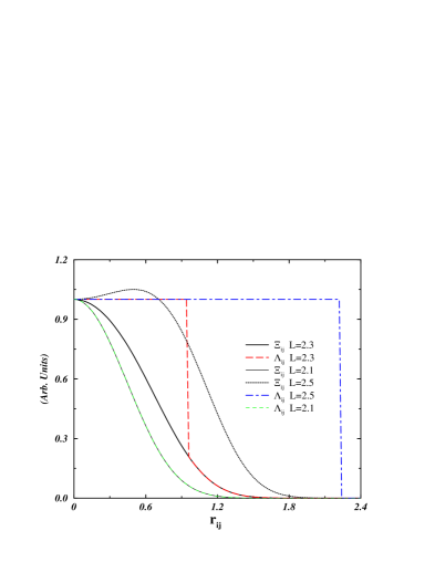
Figure 1: (color online) The off-diagonal element of $\Lambda$ and $\Xi$ ($\Lambda_{ij}$ and $\Xi_{ij}$) as a function of particle separation ($r_{ij}$) for a few selected lengths of path ($L$) at T=0.5. When the length of path is short, $\Lambda_{ij}$ and $\Xi_{ij}$ are the same. As length being longer, $\Xi_{ij}$ can be larger than one for short particle separation. In contrast, $\Lambda_{ij}$ is not larger than one for any case.

After carrying out above coarse-grained approximation, we find that, the off-diagonal element $\Xi_{\alpha\gamma}$ is a function of both $r_{\alpha\gamma}^{(M)}$ and $L_{\alpha}$, which has an explicit nonlocal form. In contrast, the off-diagonal element $A_{\alpha\gamma}$ is a local function in imaginary time. More importantly, the off-diagonal element $A_{\alpha\gamma}$ could be much larger or much smaller than 1.0, while the off-diagonal element $\Xi_{\alpha\gamma}$ is less than 1.0 when $L_{\alpha}$ is not too long (see Fig. 1). Thus, after replacing $A_{\alpha\gamma}$ with $\Xi_{\alpha\gamma}$, at least for two-particle system, a lot of sign fluctuations are well canceled. However, since the length of path could be much longer at low temperature, the off-diagonal element $\Xi_{\alpha\gamma}$ can be larger than 1.0 (see Fig. 1), which will result in the presence of negative $det\Xi$. To further reduce the negative sign, we have made the second stage of coarse-grained approximation for longer paths. Using the similar idea as above, we can replace $\Xi$ by a $N\times N$ matrix $\Lambda$,

$$\Lambda_{\alpha\gamma} =\left\{\begin{array}[]{ll}\Xi_{\alpha\gamma},forL_{\alpha}\leq L_{\alpha}^{\ast}\\ \eta(r_{\alpha\gamma}^{(M)}),forL_{\alpha}>L_{\alpha}^{\ast}\\ \end{array}\right.$$ (17)

$L_{\alpha}^{\ast}$ is a function of $r_{\alpha\gamma}^{(M)}$, which is determined by,

$$\eta(r_{\alpha\gamma}^{(M)})=\frac{\int_{L_{\alpha}^{\ast}}^{\infty}\prod_{\nu=1}^{M-1}D\vec{r}_{\alpha}^{(\nu)}\Xi_{\alpha\gamma}exp(-\beta H)}{\int_{L_{\alpha}^{\ast}}^{\infty}\prod_{\nu=1}^{M-1}D\vec{r}_{\alpha}^{(\nu)}exp(-\beta H)}$$ (18)

The above integral is made over all the configurations with $L_{\alpha}>L_{\alpha}^{\ast}$. For an arbitrary interact potential, the above integral is almost no hope to be evaluated exactly. However it can be calculated with approximations,

$$\eta(r_{\alpha\gamma}^{(M)})\approx\frac{\int_{L_{\alpha}^{\ast}}^{\infty}dL_{\alpha}\Xi_{\alpha\gamma}exp(-\frac{1}{2}\beta m\omega_{M}^{2}L_{\alpha}^{2})\Upsilon(L_{\alpha},\vec{r}_{\alpha}^{(M)})}{\int_{L_{\alpha}^{\ast}}^{\infty}dL_{\alpha}exp(-\frac{1}{2}\beta m\omega_{M}^{2}L_{\alpha}^{2})\Upsilon(L_{\alpha},\vec{r}_{\alpha}^{(M)})}.$$ (19)

In the evaluation of the above coarse-grained approximation, we have assumed that total potential energy is constant when $L_{\alpha}$ is longer than certain value, i.e, $L_{\alpha}^{\ast}$. In current work, we have taken $\eta(r_{\alpha\gamma}^{(M)})=1$ through the whole paper.

Within the current approximations, $\Lambda$ has a few advantages over the original matrix A. First, our calculations have shown that the off-diagonal element of $\Lambda$ is not larger than 1.0 anywhere (see Fig. 1), in constrast the off-diagonal element of A could be much larger than 1.0. Thus at least for two-particle system, $\Lambda$ is always non-negative, the sign problem completely vanishes. Second, different from A, $\Lambda$ is nonlocal, which depends on the whole path. The nonlocal behavior of $\Lambda$ can effectively avoid the collapse of fermion system into boson system at low temperature. At low temperature, the length of path becomes longer and longer, so the off-diagonal element of $\Lambda$ has more chance being 1.0. This situation makes $\Lambda$ have little chance being unit matrix. Our calculation also demonstrates this point. It should be pointed out that the current formula is exact for free particles (see APPENDIX).

Now we end up with the final formula for real calculations,

$$Z\cong C\int\prod_{i=1}^{N}\prod_{\nu=1}^{M}D\vec{r}_{i}^{(\nu)}det\Lambda exp[-\beta\sum_{i=1}^{N}\sum_{\nu=1}^{M}\frac{1}{2}m\omega_{M}^{2}(\vec{r}_{i}^{(\nu+1)}-\vec{r}_{i}^{(\nu)})^{2}+\sum_{\nu=1}^{M}\frac{1}{M}V(\{\vec{r}_{i}^{(\nu)}\})]$$ (20)

In real calculation, the element of $\Lambda$ is first numerically integrated. At the same time, the derivative of $\Lambda$ respective to temperature is also numerically calculated to account the contribution to thermal energy. Eq. 18 can not be directly used in standard MC, since for the fermionic systems, $det\Lambda$ is not always positive. However Eq. 18 can be integrated using modified MC technique, which is widely used previously.DeR81 ; Takahashi84 To achieve this result, we first defined pseudo-Hamiltonian, $H_{p}$, which is,

$$H_{p}=\sum_{i=1}^{N}\sum_{\nu=1}^{M}\frac{1}{2}m\omega_{M}^{2}(\vec{r}_{i}^{(\nu+1)}-\vec{r}_{i}^{(\nu)})^{2}+\sum_{\nu=1}^{M}\frac{1}{M}V(\{\vec{r}_{i}^{(\nu)}\})+ln|det\Lambda|.$$

The thermodynamic average of a physical quantity Q is

$$\langle Q\rangle=\frac{\int\prod_{i=1}^{N}\prod_{\nu=1}^{M}D\vec{r}_{i}^{(\nu)}Q(\{r_{i}^{(\nu)}\})sgn(det\Lambda)exp(-\beta H_{p}\})}{\int\prod_{i=1}^{N}\prod_{\nu=1}^{M}D\vec{r}_{i}^{(\nu)}sgn(det\Lambda)exp(-\beta H_{p}\})\})},$$ (21)

where $sgn(det\Lambda)$ stands for the sign of $det\Lambda$ at a configuration.

It needs to be pointed out that, we have used the similar technique as most pseudopotential methods,Schnitker87 ; Landman87 ; Hall88 ; Kuki87 ; Coker87 ; Bartholomew85 ; Sprik85 ; Oh98 ; Miura01 but we do not recast matrix $\Lambda$ or extend $\Lambda$ into each imaginary time.

III The Numerical Tests

To illustrate the usefulness of the current method, we have considered N interacting spinless fermions confined in a three-dimensional harmonic well, which Hamiltonian reads,

$$H=\sum_{j=1}^{N}(\frac{\vec{p}_{j}^{2}}{2m}+\frac{m\omega^{2}}{2}\vec{r}_{j}^{2})+\sum_{i<j}^{N}V(r_{ij}),$$ (22)

where m, $\vec{r}_{j}$, $\vec{p}_{j}$ and $V(r_{ij})$ are mass, positions, momenta of the particles, and the inter-particle interaction potential, respectively. For computational simplicity, the units by which $m=\hbar=k_{B}=1$ are used through the rest of this paper. In current calculations, we consider three cases, i.e, Case 1: $V(r_{ij})=0$, N=6 and $\omega^{2}=1$, no interaction between particles, reflecting a standard harmonic system; Case 2: N=6, $V(r_{ij})=-\frac{m\Omega^{2}}{2}r_{ij}^{2}$, where the interaction is also harmonic one with $\Omega^{2}=\frac{1.0}{4.0}$ and $\omega^{2}=4$; Case 3: $V(r_{ij})=\frac{q^{2}}{|\vec{r}_{i}-\vec{r}_{j}|}$, $\omega^{2}=0.320224986$, $q=1$ and N=2, interaction between particles is the Coulomb potential, the parameters correspond to hydrogen-like ion ($H^{+}$) of Kestner-Sinanoḡlu model.Kestner62 The exact results of all three cases can be found elsewhere,Kestner62 ; Brosens98 which is easy to check the validity of the current method. These models are widely used as a benchmark for checking the usefulness of various methods for sign problem, see for examples Ref.Lyubartsev ; Newman91 ; Hall88 ; Miura01

Our Metropolis MC scheme is preformed based on Eq. 19. At each step, $H_{p}$ are calculated to determine the rejection and acceptance. $det\Lambda$ is calculated by a certain algorithm with the computational cost scaled by $N^{3}$.nr This kind of numerical technique enables us to perform the fermionic simulations with reasonable computational time. There are two basic types of moves in current simulations: (1) Displacement move, where all the coordinates for a single particle are displaced uniformly; (2) Standard bisection moves.Ceperley95 ; Chakravarty The MC procedure used in this work is wildly used by others. One MC step is defined as one application of each procedure. Ten million MC steps of calculation were carried out for each temperature. For a few cases, 100 million MC steps are made to check the ergodic problem. The results agree with the short runs within the error bars. To further check the ergodic problem, the simulations are carried out by a few random generated starting configurations. All simulations converge to the same results. The energy is calculated based on the thermodynamic estimator.Ceperley95 The energies are well converged at M/$\beta$=20, 22 and 5 for case 1, 2 and 3 respectively.

The calculated thermal energy is in good agreement with the exact one for all three cases studied. In case 3, the exact energy 2.647 of Ref. Kestner62 has been almost accurately reproduced, which is 2.652$\pm$0.003 in current simulations. Fig. 2 shows the thermal energy per particle as a function of temperature for Case 1 and 2, the corresponding exact results are also shown in Fig. 2 with lines. As can be seen from the figure, the overall temperature dependence is well reproduced by current calculations. The calculated thermal energies agree very well with the exact value at low temperature. The slight deviation at high temperature is due to the fact that the first stage of approximation will result in error when the number of beads is too small, which is the case for high temperature.

We have calculated the pair correlation function (PCF) between beads, which is defined as,

$$g(r)=\langle\frac{2}{MN(N-1)}\sum_{\nu}^{M}\sum_{i}^{N-1}\sum_{j>i}^{N}\delta(r-|\vec{r}_{i}^{(\nu)}-\vec{r}_{j}^{(\nu)}|)\rangle.$$

It is known that,Miura01 comparing with boson and Boltzmann systems, the fermionic PCF has a hole around the origin, which reflects the Pauli exclusion principle. In Fig. 3, we present PCF for case 1 and 2 at temperature of 0.2. From this figure, we can see that, the pair correlation function clearly represents the effect due to the Pauli exclusion principle. The similar behaviors are observed for other temperature and systems.

The average sign reflects the signal-to-noise ratio, which directly affects calculation precision and computation time needed. The average sign is defined as $Sign=(N_{+}-N_{-})/(N_{+}+N_{-})$, where $N_{+}$ and $N_{-}$ are the total positive and negative configuration respectively. The lower panel of Fig. 4 shows the average sign of current simulations via temperature. It can be seen that, $Sign$ decreases with the decrease of the temperature. However, for the studied systems, even at lowest temperature (T=0.1), the average sign is quite high (around 0.1). We also calculated the average sign via the number of particles at T=0.5 for both case 1 and 2, which is shown in the upper panel of Fig. 4. Similarly, $Sign$ also decreases with the increase of the number of particles. Although we have not completely solved the sign problem, our approach does much improve the sign decay rate with both temperature and number of particles. Direct using of Eq. 4, $Sign$ is about 0.01 at temperature of 0.8 for case 1. And for temperature lower than 0.8, the large sign fluctuation makes MC simulation difficult to obtain any useful information. According to the data shown in Fig. 4, the maximum number of particles, which can be handled in current method, should be in order of ten. Considering both spin-up and -down, the maximum number of particles can be around twenty, which could be particularly useful for atom and molecular systems.

IV Discussion and Conclusion

In this paper, we have introduced an approach to reduce the fermion sign fluctuation in finite temperature PIMC simulations. By this method, configurations, which probably cause the sign fluctuation, are pre-calculated within two stages of coarse-grained approximations, while the rest are treated exactly. After two stages of coarse-grained approximations, at least for two-particle system, the sign problem is solved completely. Since the exchange matrix $A$ is replaced by a non-local one ($\Lambda$), the collapse of fermion system into a boson one at low temperature has been effectively avoided. The pilot calculation was performed on three model systems: six independent particles in a three-dimensional harmonic well, six interacting particles in a three-dimensional harmonic well, and hydrogen-like ion ($H^{+}$) of Kestner-Sinanoḡlu model. The calculation shows that the current approach not only dramatically drops the sign fluctuation, but also gives an excellent description to real systems. Our method could be particularly useful for atom and molecular systems. Although our approach suffers from the sign problem for large number of particles, we believe that it provide an alternative thought on the sign problem. We also believe that a similar approach can also be helpful in other path integral methods. The current formula can be easily extended to systems consisting of both spin-up and -down fermions.(see for example, Oh98 ; Takahashi )

Our approximation breaks down for systems including particles more than twenty (including both spin up and down particles). It would be possible to generalize our method for problems of larger numbers of fermions. Although we have used $\eta(r_{ij}^{(M)})=1$ through out this paper, other values are also possible. For example, if $\eta(r_{ij}^{(M)})=exp(-\alpha\frac{\beta}{2M}m\omega_{M}^{2}(r_{ij}^{(M)})^{2}$) is chosen, the current method can be more flexible. For $\alpha=0$, it is the case used in current work. For $\alpha=1$, $det\Lambda$ becomes the exact density matrix of free particles(see APPENDIX), thus the sign problem can be avoided completely. In fact, with $\alpha$ increasing from 0 to 1, the approximation becomes more and more crude, but the negative parts become less and less. To further improve the current method, a better form or value for $\eta(r_{ij}^{(M)})$ could be found. It is actually the issue on which we are working now.

APPENDIX

In this appendix, we will prove that the current formula is exact for free particles. Since the second stage of approximation is just a straightforward integration for free particles, we only prove the formula of first stage is correct for free particles. All Cartesian coordinates are equivalent for free particles, for simplicity we only prove it in one Cartesian direction, say, x.

The partition function for free particles in one dimension has the form,

$$Z=\frac{1}{N!}\int\prod_{i=1}^{N}Dx_{i}^{(M)}\rho(\{x_{i}^{(M)}\},\{x_{i}^{(M)}\})$$ (23)

where $\rho(x_{i}^{(M)},x_{i}^{(M)})$ is the density matrix, of which element with current formula reads,

$$\rho_{ij}(\{x_{i}^{M}\},\{x_{i}^{M}\})=C_{1D}\int\prod_{i=1}^{N}\prod_{\nu=1}^{M-1}Dx_{i}^{(\nu)}\Xi_{ij}^{(1D)}exp(-\beta\sum_{i=1}^{N}\frac{1}{2}m\omega_{M}^{2}L_{ix}^{2})$$ (24)

where $C_{1D}=(\frac{mM}{2\pi\beta\hbar^{2}})^{\frac{M}{2}}$, and $\Xi_{ij}^{(1D)}$ is the one-dimensional counterpart of $\Xi_{ij}$, which is

$$\Xi_{ij}^{(1D)}=\frac{\int dx_{i}^{(1)}\bar{\Delta}(L_{ix},x_{i}^{(1)},x_{i}^{(M)})e^{-\frac{1}{2}\beta m\omega^{2}_{M}((x_{i}^{(1)}-x_{j}^{(M)})^{2}-(x_{i}^{(1)}-x_{i}^{(M)})^{2})}}{\Upsilon_{1D}(L_{xi},x_{i}^{(M)})}$$ (25)

$$\Upsilon_{1D}(L_{ix},x_{i}^{(M)})=\int dx_{i}^{(1)}\bar{\Delta}(L_{ix},x_{i}^{(1)},x_{i}^{(M)})$$

Eq. 22 is only relevant to $\{L_{ix}\}$ and $\{x_{i}^{(1)}\}$, the integration over $x_{i}^{(\nu)}$ ($\nu$=1,…M-1) can be replaced by (M-1)-dimensional spherical polar coordinates, i.e, integration over $L_{ix}$ multiplying $\Upsilon_{1D}(L_{ix},x_{i}^{M})$, Eq. 22 becomes,

$$\rho_{ij}(\{x_{i}^{M}\},\{x_{i}^{M}\})\propto C_{1D}\int dL_{xi}dx_{i}^{(1)}\bar{\Delta}(L_{ix},x_{i}^{(1)},x_{i}^{(M)})$$ (26)

$$\times exp(-\frac{1}{2}\beta m\omega_{M}^{2}(L_{ix}^{2}+(x_{i}^{(1)}-x_{j}^{(M)})^{2}-(x_{i}^{(1)}-x_{i}^{(M)})^{2}))$$

Remembering for fixed $x_{i}^{(1)}$ and $x_{i}^{(M)}$, the minimum value of $L_{ix}^{2}$ equals to $(x_{i}^{(1)}-x_{i}^{(M)})^{2}\frac{M}{M-1}$. We first do the integration over variable $\{L_{ix}\}$ by change of variables as $L_{ix}^{{}^{\prime}2}=L_{ix}^{2}-(x_{i}^{(1)}-x_{i}^{(M)})^{2}\frac{M}{M-1}$, $\rho_{ij}(\{x_{i}^{M}\},\{x_{i}^{M}\})$ becomes,

$$\rho_{ij}(\{x_{i}^{M}\},\{x_{i}^{M}\})\propto C_{1D}C_{\bar{\Delta}}\frac{(\frac{M-4}{2})!}{(\frac{\beta m\omega_{M}^{2}}{2})^{\frac{M-2}{2}}}\int dx_{i}^{(1)}$$ (27)

$$\times exp(-\frac{1}{2}\beta m\omega^{2}_{M}((x_{i}^{(1)}-x_{j}^{(M)})^{2}+\frac{1}{M-1}(x_{i}^{(1)}-x_{i}^{(M)})^{2}))$$

$$=C_{1D}C_{\bar{\Delta}}\frac{(\frac{M-4}{2})!}{(\frac{\beta m\omega_{M}^{2}}{2})^{\frac{M-2}{2}}}\sqrt{\frac{2(M-1)\pi}{M\beta m\omega_{M}^{2}}}exp(-\frac{1}{2M}\beta m\omega^{2}_{M}(x_{i}^{(M)}-x_{j}^{(M)})^{2})$$

$$=C_{M}(\frac{m}{2\pi\beta\hbar^{2}})^{\frac{1}{2}}exp(-\frac{1}{2M}\beta m\omega^{2}_{M}(x_{i}^{(M)}-x_{j}^{(M)})^{2}),$$

where $C_{M}$ is an irrelevant constant. The above express is the exact formula for free particles. It needs to noted that, since we only can get the relative value for $\bar{\Delta}$, we could not obtain the absolute value of $C_{M}$. However the absolute value of $C_{M}$ is irrelevant to our calculation, which is a function of M only. Our numerical test also shows that the calculated element of density matrix based on the current formula is in excellent agreement with the exact data. In fact, the current formula must be exact for free particles, since all the approximations become exact without potential part.

Figure 2: (color online) The thermal energy of case 1 (Circle) and 2 (Squares) as a function of temperature calculated by PIMC. The solid and dash lines are the exact energies of case 1 and 2 respectively. The agreement is quite well.

Figure 3: The pair correlation functions between beads at T=0.2 for both case 1 and 2. The hole around original is the reflection of Pauli exclusion principle.

Figure 4: The average sign of case 1 (circles) and 2 (squares) via temperature (lower panel) and number of particles (upper panel) as calculated by our PIMC simulation. Sign decreases with the decrease of temperature, and the increase of number of particles.

References

• (1) D. M. Ceperley, Rev. Mod. Phys. 67, 279 (1995).
• (2) W. M. C. Foulkes et al, Rev. Mod. Phys. 73, 33 (2001).
• (3) See, e.g., Quantum Monte Carlo Methods in Condensed Matter Physics, edited by M. Suzuki (World Scientific, Singapore, 1993), and references therein.
• (4) E. Y. Loh, Jr., J. E. Gubernatis, R. T. Scalettar, S. R. White, D. J. Scalapino, and R. L. Sugar, Phys. Rev. B 41, 9301 (1990).
• (5) J. B. Anderson, J. Chem. Phys. 63, 1499(1975); 65, 4121 (1976)
• (6) D. M. Ceperley, Phys. Rev. Lett. 69, 331(1992)
• (7) D. M. Ceperley and B. J. Alder, Phys. Rev. Lett. 45, 566 (1980); J. Chem. Phys. 81, 5833 (1984).
• (8) B. Chen and J. B. Anderson, J. Chem. Phys. 102, 4491 (1995).
• (9) C. H. Mak, R. Egger and H. Weber-Gottschick, Phys. Rev. Lett. 81 4533(1998).
• (10) R. Egger, L. Mühlbacher and C. H. Mak, Phys. Rev. E 61 5961 (2000).
• (11) R. A. Chiles, G. A. Jongeward, M. A. Bolton, and P. G. Wolynes, J. Chem. Phys. 81,2039 (1984).
• (12) J. Schnitker and P. J. Rossky, J. Chem. Phys. 86, 347l (1987).
• (13) U. Landman, R. N. Barnett, C. L. Cleveland, D. Scharf, and J. Jortner, International J. Quantum Chem., Quantum Chem. Symp. 21, 573 (1987).
• (14) R. W. Hall, J. Chem. Phys. 89, 4212 (1988); J. Phys. Chem. 93,5628 (1989).
• (15) A. Kuki and P. G. Wolynes, Science 236, 1647 (1987).
• (16) D. F. Coker, B. J. Berne, and D. Thirumalai, J. Chem. Phys. 86, 5689 (1987).
• (17) J. Bartholomew, R. Hall, and B. J. Berne, Phys. Rev. B 32, 548 (1985).
• (18) M. Sprik, M. L. Klein, and D. Chandler, Phys. Rev. B 32, 545 ( 1985); Phys. Rev. B 31, 4234 (1985); J. Chem. Phys. 83,3042 ( 1985).
• (19) Ki-dong Oh and P. A. Deymier, Phys. Rev. Lett. 81, 3104 (1998); Phys. Rev. B 58, 7577 (1998).
• (20) S. Miura and S. Okazaki, J. Chem. Phys. 112, 10116 (2000); 115, 5353 (2001).
• (21) W. H. Newman and A. Kuki, J. Chem. Phys. 96, 1409(1991).
• (22) A. P. Lyubartsev, J. Phys. A: Math. Gen. 38, 6659 (2005); J. Phys. A: Math. Theor. 40, 7151 (2007).
• (23) A. G. Moreira, S. A. Baeurle and G. H. Fredrickson, Phys. Rev. Lett. 91, 150201 (2003).
• (24) S. Zhang, J. Carlson and J. E. Gubernatis, Phys. Rev. B 55, 7464(1997)
• (25) S. Zhang, Phys. Rev. Lett. 83, 2777 (1999).
• (26) P. Henelius and A. W. Sandvik Phys. Rev. B 62 1102(2000).
• (27) R. P. Pathria, Statistical Mechanics, (Elsevier(Singapore) Pte Ltd. 2003), pp. 504.
• (28) See, for example, W. H. Press, S. A. Teukolsky, W. T. Vetterling, and B. P. Flannery, Numerical Recipes in Fortran, 2nd ed. (Cambridge U.P., New York, 1992).
• (29) H. De Raedt and A. Lagendijk, Phys. Rev. Lett. 46, 77 (1981).
• (30) M. Takahashi and M. Imada, J. Phys. Soc. Jpn. 53, 963 (1984).
• (31) N. R. Kestner and O. Sinanoḡlu, Phys. Rev. 128, 2687 (1962).
• (32) F. Brosens, J. T. Devreese and L. F. Lemmens, Phys. Rev. E 57, 3871 (1998).
• (33) C. Chakravarty, M. C. Gordillo and D. M. Ceperley, J. Chem. Phys. 109, 2124 (1998).
• (34) M. Takahashi and M. Imada, J. Phys. Soc. Jpn. 53, 963 (1984).
Refer to caption