Phonon distributions of a single bath mode coupled to a quantum dot

Abstract

The properties of an unconventional, single mode phonon bath coupled to a quantum dot, are investigated within the rotating wave approximation. The electron current through the dot induces an out of equilibrium bath, with a phonon distribution qualitatively different from the thermal one. In selected transport regimes, such a distribution is characterized by a peculiar selective population of few phonon modes and can exhibit a sub-Poissonian behavior. It is shown that such a sub–Poissonian behavior is favored by a double occupancy of the dot. The crossover from a unequilibrated to a conventional thermal bath is explored, and the limitations of the rotating wave approximation are discussed.

1 Introduction

The study of dissipation and decoherence is a central problem in the description of solid state systems both from the fundamental and the applicative point of view. One of the most popular models, employed to describe dissipation, is the one introduced by Caldeira and Leggett [1] in which the dissipative environment is a bath of harmonic oscillators whose fluctuations obey Gaussian statistics, linearly coupled to the system under consideration [2, 3]. While this model is reasonable to describe the dissipation induced by large environments, such as equilibrium Fermi reservoirs, it is becoming clear that possible sources of decoherence do not necessarily fall into this category for nanodevices such as quantum dots and qubits. Solid state nanocircuits typically suffer from discrete noise, often originated from background charge fluctuations. Single/few impurities behaving either like random telegraph noise sources [4] or being entangled with the device have been recently observed [5] in different setups. The resulting non-gaussian effects can only be predicted introducing non-linear bath models [6]. In addition, the excellent control recently achieved in circuit-QED experiments [7] has paved the way to the observation of quantum effects originating from the coupling of multilevel nanodevices to a single harmonic mode of a high-Q cavity resulting in a effective bath having a structured power spectrum [8]. All these mechanisms deviate from the canonical Caldeira and Leggett description and are examples of unconventional dissipative baths.

The coupling to an unconventional dissipative bath arises also in the case of a nanoresonator coupled to a quantum dot, where electrons are coupled to few or even a single phonon mode [9]. An experimental realization of such a system is the phonon cavity studied by Weig et al. [10]. Here, the coupling to the single bath mode induces sizable effects on the transport properties of the dot, with the appearance of peaks in the conductance spectrum when the energy of tunneling electrons matches the energy of the phonon mode. A similar phenomenon occurs in a oscillating C₆₀ molecule contacted by gold leads [11].

Often, in these cases both the leads bath and the localized bath mode are assumed to be in their thermal equilibrium [12]. However, there are several situations in which this assumption is not justified especially for the localized mode. For example, in suspended carbon nanotubes, the electrons are coupled with a single longitudinal stretching [13], or to a radial breathing [14] phonon mode. The unconventional single mode bath is driven out of equilibrium by the electron current and it induces the appearance of peculiar negative differential conductance traces [15, 16]. Another example is that of the superconducting single electron transistor coupled to a single–mode nanoresonator studied by Naik et al. [17], where the back–action exerted by the single electron transistor cools down the phonon mode below the temperature of the environment. Then, it may be necessary to treat the leads and the single mode on a different footing. While the leads degrees of freedom can be assumed in their thermal equilibrium and are traced out in the usual way, the coupled dynamics of the electrons and the localized boson is treated without assuming a priori a distribution for the localized mode.

Such a issue will be the subject of investigation in this work. We will consider a spin degenerate single level quantum dot with finite Coulomb repulsion coupled to two external environments:

($i$) a pair of Fermi leads, described by a standard Caldeira Leggett model,

($ii$) an unconventional non–relaxed single phonon bath.

The transport properties of such a system have been theoretically analyzed both in the sequential tunneling and in the cotunneling regime [15, 18, 19, 20, 21]. The behavior strongly differs with respect to the one obtained for a system coupled to an equilibrated localized phonon mode [18]. In the sequential tunneling regime, besides the negative differential conductance mentioned above, the zero–frequency shot noise $S$ has been found to be even more sensitive to the bath properties [18]. In the case of strong coupling to an out of equilibrium phonon bath, a super–Poissonian shot noise $S>2eI$ ($-e$ is the electron charge, $I$ the corresponding current) has been predicted [19]. On the other hand, for a thermal bath, sub–Poissonian shot noise $S\leq 2eI$ is always found [20]. In the cotunneling regime, vibrational absorption sidebands occur within the Coulomb–blockaded regime, which disappear for the case of a single bath in thermal equilibrium [19, 21, 14]. This further confirms the importance of such a unequilibrated phonon bath to describe experimental systems.

In order to consider the coherent dynamics of the quantum dot with the single mode bath one can derive a generalized master equation within the Born–Markov approximation for the reduced density matrix of the system and the localized bath, by tracing out the leads bath. Such an approach has been employed already in the past for describing systems such as a metallic [22] or a superconducting single electron transistor [23].

Since the transport properties have been already studied in great details, we will concentrate on the steady state out of equilibrium phonon distribution of the bath ($ii$) induced by the tunneling electrons, which in the past has received much less attention [18, 24, 23, 27]. In particular, we will analyze the phonon Fano factor

$$F_{ph}=\frac{\mathrm{var}(l)}{\langle l\rangle}=\frac{\langle l^{2}\rangle-\langle l\rangle^{2}}{\langle l\rangle}\,,$$ (1)

defined as the ratio between the variance of the phonon occupation number $\mathrm{var}(l)$ and the average occupation number $\langle l\rangle$. The Fano factor brings information about the statistics of the single phonon bath mode. For a thermally equilibrated bath, one always obtains a super–Poissonian Fano factor $F_{ph}>1$. Such a super–Poissonian value is typical for “classical” boson distributions, as for example for photons in classical light [28]. As it will be shown later, in most of the transport regimes, out of equilibrium bath distributions arise which, although being strongly different from a thermal distribution, display a super–Poissonian character. However, it is possible to find particular transport regimes in which $F_{ph}<1$, corresponding to peculiar bath distributions [23, 27]. This case is analogous to that of the reduced photon fluctuation found in quantum non–classical radiation [29, 30].

Our main results are the following. In the regime where the single bath mode oscillations are much faster than the average electron dwell time, we adopt the rotating wave approximation and we investigate the phonon Fano factor. We identify the transport regimes where a sub–Poissonian single mode bath occurs for the case of a single occupancy of the dot. For a double occupancy, additional transport regions in which $F_{ph}<1$ occurs. We evaluate the “stability boundary” of the sub–Poissonian bath as a function of tunnel barriers asymmetry and coupling strength with the bath mode, finding that $F_{ph}<1$ is destroyed for increasing damping of the single mode bath. Finally, we present some preliminary results on the effects of the coherent phonon bath dynamics occurring when the oscillation time of the localized mode is of the same order or smaller than the electron tunneling time.

2 Model and methods

2.1 The system and its environments

We model the system as a small quantum dot, with an average level spacing of the same order than the charging energy, described as a spin–degenerate single level with on–site Coulomb repulsion [31]

$$H_{s}=\xi n-en\frac{C_{g}}{C}V_{g}+\frac{U}{2}n(n-1)\,.$$ (2)

Here, $\xi$ is the single energy level, $n=\sum_{\sigma=\pm}n_{\sigma}$ is the total occupation number with $n_{\sigma}=d^{\dagger}_{\sigma}d_{\sigma}$ the occupation of spin $\sigma=\pm 1$ (units $\hbar/2$), and $d_{\sigma}$ ($d^{\dagger}_{\sigma}$) are the fermionic annihilation (creation) operators. The second term in Eq. (2) is the coupling to an external gate voltage $V_{g}$, with $-e$ the electron charge, $C_{g}$ the gate capacitance, and $C=e^{2}/U$ the dot capacitance. Choosing as a reference level $\xi=U/2$ one has $H_{s}=\epsilon n+Un(n-1)/2$ with $\epsilon=U(1-2n_{g})/2$ written in terms of the number of charges induced by the gate $n_{g}=C_{g}V_{g}/e$. Note that the choice of $\xi$ determines the values of $n_{g}$ for which resonance between the $n$, $n+1$ states occur: a different choice of reference for $\xi$ would simply result in a shift of $n_{g}$.

The system is coupled to two dissipative baths with Hamiltonians ($\hbar=1$)

$$H_{b}^{(1)}=\omega_{0}\ b^{\dagger}b\,;\;\qquad H_{b}^{(2)}=\!\!\!\!\sum_{\alpha=L,R,k,\sigma=\pm}\varepsilon_{k}\ c^{\dagger}_{\alpha,k,\sigma}c_{\alpha,k,\sigma}\,.$$ (3)

Here, $H_{b}^{(1)}$ describes the harmonic oscillator single bath mode with frequency $\omega_{0}$, and $H_{b}^{(2)}$ represents the external left ($L$) and right ($R$) leads of noninteracting electrons with fermionic operators $c_{\alpha,k,\sigma}$ and $c^{\dagger}_{\alpha,k,\sigma}$. The localized phonon mode is undamped, a discussion of possible damping effects is deferred to Sec. 4.1. The leads are assumed in thermal equilibrium with respect to their electrochemical potential $\mu_{L,R}=\mu_{0}\pm eV/2$, where $V$ is the applied voltage, and $\mu_{0}$ is the reference chemical potential. The noninteracting Fermi leads can be mapped onto a ohmic dissipative bath within the Caldeira Leggett formalism [3]. More detailed models, involving a anharmonic [24] or distorted [25] oscillator or the presence of interacting Luttinger liquid leads [26], which have been studied in the past especially concerning their transport properties, will not be addressed here.

The coupling of the system with the single-mode bath is linear in the oscillator coordinate and in the effective charge $n-n_{g}$ on the dot

$$H_{sb}^{(1)}=\sqrt{\lambda}\omega_{0}(b+b^{\dagger})(n-n_{g})\,.$$ (4)

This describes realistic situations such as a single electron transistor capacitively coupled to a vibrating, charged gate [32, 33]. The tunneling Hamiltonian

$$H_{sb}^{(2)}=\sum_{\alpha=L,R}t_{\alpha}\sum_{k,\sigma=\pm}c^{\dagger}_{\alpha,k,\sigma}d_{\sigma}+h.c.\,.$$ (5)

represents the coupling of the dot with the external leads, through tunneling amplitudes $t_{L}$ and $t_{R}$. In the following, a trace over the leads degrees of freedom will be performed.

The full dynamics of the single mode will be retained, and its degrees of freedom will not be traced away. It is possible to diagonalize exactly the Hamiltonian representing the dot coupled to single phonon mode

$$H_{\lambda}=H_{s}+H_{b}^{(1)}+H_{sb}^{(1)}\,,$$ (6)

by means of the Lang–Firsov polaron transformation [18], with generator $\mathcal{U}=\exp{[-\eta(b-b^{\dagger})]}$, and $\eta=\sqrt{\lambda}(n-n_{g})$. The transformed operators, denoted by an overbar $\bar{\mathcal{O}}=\mathcal{U}\mathcal{O}\mathcal{U}^{\dagger}$, are $\bar{b}=b-\eta$ and $\bar{d}_{\sigma}=d_{\sigma}\exp{\left[\sqrt{\lambda}(b-b^{\dagger})\right]}$, while $\bar{n}=n$. Upon transformation, we have

$$\bar{H}_{\lambda}=\bar{\epsilon}n+\frac{\bar{U}}{2}n(n-1)+\omega_{0}l\,,$$ (7)

with renormalized level position $\bar{\epsilon}$ and Coulomb repulsion $\bar{U}$

$$\bar{\epsilon}=\frac{\bar{U}}{2}(1-2n_{g});\qquad\bar{U}=U-2\lambda\omega_{0}\,.$$ (8)

The eigenvectors of Eq. (7) are denoted by $|n,l\rangle$, with energy $E_{n,l}$. Note that the polaronic renormalization of the Coulomb interaction may lead to two qualitatively different physical scenarios for $\bar{U}\lessgtr 0$ or equivalently $\lambda\gtrless U/2\omega_{0}$. The regime $\bar{U}<0$, where the single occupation is always forbidden and the sequential transport is blocked, has been considered by several authors [34, 35, 36]. In the present paper, we will consider the opposite case with $\bar{U}>0$ treating the sequential tunneling regime.

Finally, the transformed tunneling Hamiltonian is

$$\bar{H}_{sb}^{(2)}=\sum_{\alpha=L,R}t_{\alpha}e^{\sqrt{\lambda}(b-b^{\dagger})}\sum_{k,\sigma=\pm}c^{\dagger}_{\alpha,k,\sigma}d_{\sigma}+h.c.\,,$$ (9)

with an the explicit dependence on the oscillator variables.

2.2 Generalized master equation

The dynamics of the dot and single bath mode can be described in terms of the reduced density matrix ${\rho}(t)$, defined as the trace over the leads bath of the total density matrix $\rho_{tot}(t)$: ${\rho(t)}=\mathrm{Tr}_{l}\{{\rho}_{tot}(t)\}$. In the following we will mainly work in the polaron frame with the density matrix denoted by $\bar{\rho}(t)$, the evolution in the original frame being easily traced back via the canonical transformation $\rho(t)=\mathcal{U}^{\dagger}(t)\bar{\rho}(t)\mathcal{U}(t)$.

We will consider the regime of weak tunneling, treating $\bar{H}_{sb}^{(2)}$ in Eq. (5) to lowest order, and assume the characteristic memory time of the leads much shorter than the response time of the dot interacting with the localized phonon bath. This allows to treat the dynamics in the Born-Markov approximation [37] leading to a generalized master equation (GME). Assuming a factorized total density $\bar{\rho}_{tot}(t)=\bar{\rho}(t)\otimes\rho_{l}(0)$ with the leads in thermal equilibrium with respect to corresponding chemical potential $\mu_{L,R}$: $\rho_{l}(0)=\rho_{L}(0)\otimes\rho_{R}(0)$, the time evolution in the interaction picture (denoted with the subscript “$I$”) is

$$\dot{\bar{\rho}}_{I}(t) =-\sum_{\sigma=\pm}\int_{0}^{\infty}{\rm d}\tau\left\{[Q_{I,\sigma}(t),Q^{\dagger}_{I,\sigma}(t-\tau)\bar{\rho}_{I}(t)]K^{+}(\tau)\right.$$ (10)

$$- [Q_{I,\sigma}(t),\bar{\rho}_{I}(t)Q^{\dagger}_{I,\sigma}(t-\tau)]K^{-}(\tau)+[Q^{\dagger}_{I,\sigma}(t),Q_{I,\sigma}(t-\tau)\bar{\rho}_{I}(t)]K^{-}(-\tau)$$

$$- \left.[Q^{\dagger}_{I,\sigma}(t),\bar{\rho}_{I}(t)Q_{I,\sigma}(t-\tau)]K^{+}(-\tau)\right\}\,.$$

Here, we defined the operator $Q_{\sigma}=e^{\sqrt{\lambda}(b-b^{\dagger})}d_{\sigma}$ and the leads correlation functions

$$K^{\pm}(\tau)=\sum_{\alpha,k}|t_{\alpha}|^{2}e^{i\varepsilon_{k}\tau}f^{\pm}_{\alpha}(\varepsilon_{k})\,,$$ (11)

with $f^{+}_{\alpha}(\varepsilon)=1/\{1+\exp{[\beta(\varepsilon-\mu_{\alpha})]}\}$ the Fermi distribution of lead $\alpha$ and $f^{-}_{\alpha}(\varepsilon)=1-f^{+}_{\alpha}(\varepsilon)$. Note that the correlation function $K^{+}(\tau)$ can be cast into the form [38, 39]

$$K^{+}(\tau)=\nu\sum_{\alpha}|t_{\alpha}|^{2}e^{i\mu_{\alpha}\tau}\omega_{c}e^{-W(\tau)}\,,$$ (12)

where $\nu$ is the leads density of states and

$$W(\tau)=\int_{0}^{\infty}\mathrm{d}\omega\ \frac{J(\omega)}{\omega^{2}}\left\{[1-\cos{(\omega\tau)}]\coth{\left(\frac{\beta\omega}{2}\right)}+i\sin(\omega\tau)\right\}\,,$$ (13)

represents the dissipative kernel of a set of harmonic oscillators with ohmic spectral density $J(\omega)=\omega e^{-\omega/\omega_{c}}$, and frequency cutoff $\omega_{c}$ [3]. Expression (12) clarifies the connection between the electronic leads and the bosonic modes of the Caldeira Leggett model.

The above approximations allow to describe the dynamics of the dot in the so called sequential tunneling regime. They are typically valid for temperatures larger than the level broadening induced by tunneling $k_{B}T\gg\Gamma_{L}+\Gamma_{R}$, with $\Gamma_{\alpha}=2\pi\nu|t_{\alpha}|^{2}$. At lower temperatures, coherences between the leads and the dot play a crucial role [18]. These effects will be not discussed in this work.

It is convenient to project Eq. (10) on the eingenstates of the Hamiltonian (7) and perform the time integrations with the aid of $\int_{0}^{\infty}\mathrm{d}\tau\ e^{iE\tau}=\pi\delta(E)+i\mathrm{P.V.}(1/E)$. In the following, terms stemming from the principal value are neglected since they lead to small corrections in the perturbative regime [22, 40]. Denoting with $\bar{\rho}_{I,qq^{\prime}}^{n}(t)=\langle n,q|\bar{\rho}_{I}(t)|n,q^{\prime}\rangle$ the GME has the compact form (here and in the following, $0\leq n\leq 2$ unless stated otherwise)

$$\!\!\!\!\!\!\!\!\!\!\!\!\!\!\!\!\!\dot{\bar{\rho}}_{I,qq^{\prime}}^{n}(t) = \sum_{k=\pm 1\atop 0\leq n+k\leq 2}\sum_{p,p^{\prime}}\left\{z_{n+k}X^{n+k,n}_{q^{\prime}p^{\prime}}X^{n+k,n}_{qp}(\gamma^{n+k,n}_{pq}+\gamma^{n+k,n}_{p^{\prime}q^{\prime}})\bar{\rho}^{n+k}_{I,pp^{\prime}}(t)e^{-i(\omega_{q^{\prime}q}+\omega_{pp^{\prime}})t}\right.$$ (14)

$$- \left.z_{n}X^{n,n+k}_{p^{\prime},p}\gamma^{n,n+k}_{pp^{\prime}}[X^{n,n+k}_{p^{\prime}q}\bar{\rho}^{n}_{I,pq^{\prime}}(t)e^{-i\omega_{pq}t}+X^{n,n+k}_{p^{\prime}q^{\prime}}\bar{\rho}^{n}_{I,qp}(t)e^{-i\omega_{q^{\prime}p}t}]\right\}\,.$$

Here we defined $\omega_{pp^{\prime}}=\omega_{0}\cdot(p-p^{\prime})$, with the indexes $p,p^{\prime},q,q^{\prime}$ that run over $[0,\infty)$. The factors $z_{0}=z_{2}=2$, $z_{1}=1$ arise due to the spin degeneracy of the state $n=1$. Furthermore, it is

$$\gamma_{pq}^{n,n+1}=\sum_{\alpha}\frac{\Gamma_{\alpha}}{2}f_{\alpha}^{+}(E_{n+1,q}-E_{n,p})\quad\quad\quad\gamma_{pq}^{n+1,n}=\sum_{\alpha}\frac{\Gamma_{\alpha}}{2}f_{\alpha}^{-}(E_{n+1,p}-E_{n,q})$$ (15)

and we have introduced

$$X^{n+1,n}_{qq^{\prime}}=X_{qq^{\prime}}\quad\quad\quad X^{n,n+1}_{qq^{\prime}}=X_{q^{\prime},q}$$ (16)

with $X_{qq^{\prime}}=\langle n,q|e^{\sqrt{\lambda}(b-b^{\dagger})}|n,q^{\prime}\rangle$ the Franck–Condon factors, given by

$$X_{qq^{\prime}}=e^{-\lambda/2}\sqrt{\frac{q_{<}!}{q_{>}!}}L_{q_{<}}^{|q^{\prime}-q|}(\lambda)\left[\mathrm{sgn}(q^{\prime}-q)\sqrt{\lambda}\right]^{|q^{\prime}-q|}\,,$$ (17)

where $q_{<}=\mathrm{min}\{q,q^{\prime}\}$, $q_{>}=\mathrm{max}\{q,q^{\prime}\}$ and $L_{\mu}^{\nu}(\lambda)$ is the generalized Laguerre polynomial. They satisfy the relation $X_{qq^{\prime}}^{2}=X_{q^{\prime}q}^{2}$.

In the Schrödinger representation, Eq. (14) becomes

$$\!\!\!\!\!\!\!\!\!\!\!\!\!\!\dot{\bar{\rho}}_{qq^{\prime}}^{n}(t) = -i\omega_{qq^{\prime}}\bar{\rho}_{qq^{\prime}}^{n}(t)+\!\!\!\sum_{k=\pm 1\atop 0\leq n+k\leq 2}\!\!\sum_{p,p^{\prime}}\left\{z_{n+k}X^{n+k,n}_{q^{\prime}p^{\prime}}X^{n+k,n}_{qp}(\gamma^{n+k,n}_{pq}+\gamma^{n+k,n}_{p^{\prime}q^{\prime}})\bar{\rho}^{n+k}_{pp^{\prime}}(t)\right.$$ (18)

$$- \left.z_{n}X^{n,n+k}_{p^{\prime}p}\gamma^{n,n+k}_{pp^{\prime}}[X^{n,n+k}_{p^{\prime}q}\bar{\rho}^{n}_{pq^{\prime}}(t)+X^{n,n+k}_{p^{\prime}q^{\prime}}\bar{\rho}^{n}_{qp}(t)]\right\}\,.$$

The GME (18) is an infinite set of coupled linear differential equations which cannot be solved analytically under general conditions. We numerically solve the system truncating the harmonic oscillator Hilbert space to increasingly larger sizes $q,q^{\prime}\lesssim 70$, until convergence is achieved.

2.3 Rotating wave approximation

In the regime of fast vibrational motion of the localized bath, $\omega_{0}\gg\Gamma_{L},\Gamma_{R}$, one can perform the rotating wave approximation (RWA), neglecting terms in Eq. (14) with an explicit oscillatory exponential time dependence [37]. In the Schrödinger representation, this leads to a GME of the form

$$\!\!\!\!\!\!\!\!\!\!\!\!\!\!\!\!\!\!\!\!\!\!\!\dot{\bar{\rho}}_{qq^{\prime}}^{n}(t) = -i\omega_{qq^{\prime}}\bar{\rho}_{qq^{\prime}}^{n}+\sum_{k=\pm 1\atop 0\leq n+k\leq 2}\left\{\sum_{p=-q_{<}}^{\infty}z_{n+k}X^{n+k,n}_{q,q+p}X^{n+k,n}_{q^{\prime},q^{\prime}+p}\bar{\rho}^{n+k}_{q+p,q^{\prime}+p}\right.(\gamma^{n+k,n}_{q+p,q}+\gamma^{n+k,n}_{q^{\prime}+p,q^{\prime}})$$ (19)

$$\left.-z_{n}\bar{\rho}^{n}_{q,q^{\prime}}\sum_{p=0}^{\infty}\left[(X^{n,n+k}_{pq^{\prime}})^{2}\gamma^{n,n+k}_{q^{\prime}p}+(X^{n,n+k}_{pq})^{2}\gamma^{n,n+k}_{qp}\right]\right\}\,.$$

Note that in the RWA the density matrix elements $\bar{\rho}_{qq^{\prime}}^{n}$ and $\bar{\rho}_{ll^{\prime}}^{n^{\prime}}$ are coupled only if $l^{\prime}-l=q^{\prime}-q$. This implies that the diagonal elements $\bar{\rho}_{qq}^{n}(t)$ are decoupled from the off-diagonal ones. In addition, the non diagonal elements vanish in the stationary regime, $\bar{\rho}^{n}_{l,l^{\prime}\neq l}(t\to\infty)\to 0$, as a difference with the coherent regime (see section 4.2). Hence, within the RWA all the stationary properties are determined by the diagonal occupation probabilities $\bar{\rho}_{qq}^{n}\equiv\bar{P}_{nq}$ and Eq. (19), in the stationary limit, assumes the form of a standard rate equation

$$z_{n}\bar{P}_{nq}\sum_{k=\pm 1\atop 0\leq n+k\leq 2}\sum_{p=0}^{\infty}\Gamma_{qp}^{n,n+k}-\sum_{k=\pm 1\atop 0\leq n+k\leq 2}\sum_{p=0}^{\infty}z_{n+k}\bar{P}_{n+k,p}\Gamma^{n+k,n}_{pq}=0$$ (20)

$$\Gamma^{nn^{\prime}}_{pq}=\Gamma^{nn^{\prime}}_{L,pq}+\Gamma^{nn^{\prime}}_{R,pq}=2X_{p,q}^{2}\gamma^{nn^{\prime}}_{pq}$$ (21)

with $\Gamma^{nn^{\prime}}_{pq}$ the tunneling rates for the transition $|n,p\rangle\to|n^{\prime},q\rangle$ and $\Gamma_{\alpha,pq}^{nn^{\prime}}$ the tunneling rate on barrier $\alpha$. We specify here the energy regions where tunneling processes with rates $\Gamma^{nn^{\prime}}_{pq}$ are allowed (i.e. $\Gamma^{nn^{\prime}}_{pq}\neq 0$) for temperatures low enough that the Fermi function can be approximated as a step, $T\ll\omega_{0}/k_{B}$. From the definition (15) follows

$$\Gamma_{pq}^{n,n+1}\neq 0\ \Rightarrow \ E_{n+1,q}-E_{n,p}\pm eV/2\leq 0$$ (22)

$$\Gamma_{pq}^{n+1,n}\neq 0\ \Rightarrow \ E_{n+1,p}-E_{n,q}\pm eV/2\geq 0\,,$$ (23)

with the $+$ ($-$) sign for a tunneling event on the right (left) barrier. The Franck Condon factors in the tunneling rates Eq.(21) are responsible for two important effects:

($i$) suppression of all the tunneling rates by a factor $e^{-\lambda}$,

($ii$) non–trivial dependence on the phonon indexes $p$, $q$.

In particular, for moderate interactions $\lambda\lesssim 1$, transitions which conserve or change slightly the phonon number have the largest rate and, among these, the ones involving small $p$ and $q$ are dominant. Vice versa, for $\lambda\gg 1$, transitions with a large change in the phonon number are favored. These considerations will play an important role in explaining both the transport properties and the characteristics of the single mode bath.

Finally, the stationary current can be expressed in terms of the occupation probabilities as follows

$$I=-e\sum_{n=0,1}\sum_{q,q^{\prime}}\left[z_{n}\bar{P}_{nl}\Gamma_{L,qq^{\prime}}^{n,n+1}-z_{n+1}\bar{P}_{n+1,l}\Gamma_{L,qq^{\prime}}^{n+1,n}\right]\,,$$ (24)

note that $I$ is independent on the position.

In order to obtain the stationary solution of the phononic populations, we numerically solved Eq. (20) for a sufficiently large set of harmonic oscillator states with $q\lesssim 60$, which guarantees a fair convergence. A discussion of the range of validity of this approximation will be presented in Section 4.2.

3 Results

In the following we will present several effects induced by the coupling of the quantum dot with the unequilibrated single bath mode. We will consider the regime $k_{B}T\ll\omega_{0}$ where the quantization effects of the phonon mode are more visible.

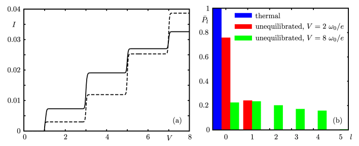
Figure 1: (a) Current $I$ (units $-e\Gamma_{L}$) as a function of $V$ (units $\omega_{0}/e$) for an unequilibrated (solid) or a thermal (dashed) phonon bath, for $n_{g}=0.525$, $A=0.01$, $\lambda=3$, $k_{B}T=0.01\ \omega_{0}$, $\bar{U}=\ 20\ \omega_{0}$ and $\Gamma_{L}=10^{-3}\omega_{0}$. (b) Phonon distributions $\bar{P}_{l}$, as a function of $l$, for the cases of a thermal bath (blue) and an unequilibrated bath calculated for $eV=2\ \omega_{0}$ (red) and $eV=8\ \omega_{0}$ (green), all other parameters as in panel (a).

Figure 1(a) shows the current $I$, numerically evaluated from Eq.(24) in the RWA, as a function of voltage in the presence of an asymmetry $A=|t_{R}|^{2}/|t_{L}|^{2}<1$. Two different conditions of the single bath mode are considered: a completely out of equilibrium distribution $\bar{P}_{l}$, determined by solving the rate equations (20), and a thermal distribution $\bar{P}_{l}^{(th)}$

$$\bar{P}_{l}=\sum_{n}\bar{P}_{nl}\,;\qquad\bar{P}_{l}^{(th)}=e^{-l\beta\omega_{0}}(1-e^{-\beta\omega_{0}})\,,$$ (25)

and $\beta=(k_{B}T)^{-1}$. For $V<\omega_{0}/e$, the dot is in the Coulomb blockade regime. For increasing $V$, steps in the current reflect phonon excitations in the bath. The solid line is the result with $\bar{P}_{l}$, the dashed line displays the current obtained imposing a thermal distribution of the bath mode. The corresponding phonon distributions $\bar{P}_{l}$ deviates considerably from $\bar{P}_{l}^{(th)}$, as shown in Fig. 1(b). While $\bar{P}_{l}^{(th)}$ at $T\ll\omega_{0}/k_{B}$ is almost concentrated at $l=0$, the unequilibrated distributions are broader.

The behavior of the current is qualitatively different, depending on the bath conditions. In particular, for $V<5\ \omega_{0}/e$ the current in the equilibrated case is smaller than for an unequilibrated phonon bath while for $V>\ 7\omega_{0}/e$ the situation is reversed [18, 20]. This fact can be explained as follows. For $\lambda>1$, as in the case of Fig. 1(a), the dominant transition involves $l=0\to\mathrm{int}(\lambda)$ [20], as a consequence of the Franck Condon factors (17). For the parameters in the figure, it corresponds to the transition $l=0\to 3$, which is open only for $V>5\omega_{0}$ as can be checked by inspecting Eqs. (22),(23). A large occupation of the states with $l=0$ leads therefore to an increase of the current. This explains why, for large voltages $V>7\omega_{0}/e$, in the case of a thermal distribution $\bar{P}_{l}^{(th)}$ one obtains a larger current with respect to the unequilibrated case where a broader phonon distribution implies a smaller $\bar{P}_{0}$ [20]. Vice versa, for $V<5\ \omega_{0}/e$ only small tunneling rates with $\Delta l\leq 2$ are open, therefore the larger the number of transport channels, the larger is the current. In the case of a thermal bath only transitions originating from $l=0$ can contribute to the current, while in the unequilibrated case also transitions starting from $l=1$ and $l=2$ states contribute, resulting in a higher current with respect to the equilibrated case.

Also the current fluctuations display deviations (not shown here): in the unequilibrated case a super–Poissonian current noise appears, while for a thermal bath one obtains a sub–Poissonian noise [19, 20]. These topics have been studied in great details [15, 18, 19, 20, 21], thus we will not repeat here the analysis of transport properties induced by the unconventional localized mode.

Instead, we will focus on the properties of the single bath mode, and we will characterize the out of equilibrium phonon distribution induced by the current flow. In particular, we will analyze the Fano factor. The averages involved in Eq. (1) are equivalently defined in the original frame or in the polaron one as $\langle\mathcal{O}\rangle=\mathrm{Tr}\{\mathcal{O}\rho\}=\mathrm{Tr}\{\bar{\mathcal{O}}\bar{\rho}\}$ with the trace performed over the degrees of freedom of the system and of the single bath mode. Since operators in the polaron frame are expressed in terms of the ones in the original frame, it will be particularly useful to introduce the hybrid average $\langle\mathcal{O}\rangle_{\bar{\rho}}=\mathrm{Tr}\{\mathcal{O}\bar{\rho}\}$. With respect to this average the above occupation number and variance are given by ($\eta=\sqrt{\lambda}(n-n_{g})$)

$$\langle l\rangle = \langle l\rangle_{\bar{\rho}}-\langle\eta x\rangle_{\bar{\rho}}+\langle\eta^{2}\rangle_{\bar{\rho}}$$ (26)

$$\langle l^{2}\rangle = \langle l^{2}\rangle_{\bar{\rho}}+\langle\eta^{4}\rangle_{\bar{\rho}}+\langle\eta^{2}x^{2}\rangle_{\bar{\rho}}+2\langle\eta^{2}l\rangle_{\bar{\rho}}-2\langle\eta^{3}x\rangle_{\bar{\rho}}-\langle\eta\{l,x\}\rangle_{\bar{\rho}}\,,$$ (27)

where $\{a,b\}=ab+ba$ and $x=b+b^{\dagger}$. Note that the Fano factor can also be connected to the Mandel parameter $\mathcal{Q}=F_{ph}-1$ [41], introduced in quantum optics to discriminate the sub–Poissonian statistics and photon antibunching [29, 30].

We point out here that in the case of a thermally equilibrated bath, with a diagonal density matrix Eq. (25) right side, one has $F_{ph}>1$ . As we will see below, deviations from an equilibrated bath usually result in super–Poissonian distributions. However, in special transport regimes it is possible to obtain peculiar distributions with a sub–Poissonian character.

3.1 Single occupancy

We start from the case $\bar{U}\gg\omega_{0}$ within the RWA. In this regime the dot, around the resonance condition $n_{g}\approx 1/2$, has a single occupancy with $n=0,1$ and shows qualitatively similar behavior to that discussed in Ref. [27], where $\bar{U}\to\infty$. Within the RWA, the Fano factor is simplified since some averages in (26) and (27) vanish due to the diagonal form of the density matrix. It is convenient to express $F_{ph}$ in terms of the numerator of the Mandel parameter $F_{ph}=1+\mathcal{Q}_{num}/\langle l\rangle$ where

$$\mathcal{Q}_{num} = \mathcal{Q}_{\bar{\rho}}+4\langle\eta^{2}l\rangle_{\bar{\rho}}-2\langle\eta^{2}\rangle_{\bar{\rho}}\langle l\rangle_{\bar{\rho}}+\langle\eta^{4}\rangle_{\bar{\rho}}-\langle\eta^{2}\rangle_{\bar{\rho}}^{2}$$ (28)

$$\mathcal{Q}_{\bar{\rho}} = \langle l^{2}\rangle_{\bar{\rho}}-\langle l\rangle_{\bar{\rho}}^{2}-\langle l\rangle_{\bar{\rho}}\,.$$ (29)

Here, we have separated a contribution, $\mathcal{Q}_{\bar{\rho}}$, depending only on the phonon distribution, and terms related to charge fluctuations on the dot (terms in $\eta^{2}$ and $\eta^{4}$). In general, one has $\mathcal{Q}_{num}\gtrless 0$ and $\mathcal{Q}_{num}>\mathcal{Q}_{\bar{\rho}}$ [27]. The necessary condition to have $F_{ph}<1$ is $\mathcal{Q}_{\bar{\rho}}<0$. However, this does not guarantee sub-Poissonian behavior since the variance $\langle\eta^{4}\rangle_{\bar{\rho}}-\langle\eta^{2}\rangle_{\bar{\rho}}^{2}$, being definite positive, could drive $F_{ph}>1$.

The quantity $\mathcal{Q}_{\bar{\rho}}$ in (29) is expressed in terms of the phonon distribution $\bar{P}_{l}$ in Eq. (25) as follows

$$\mathcal{Q}_{\bar{\rho}}=\sum_{l}\bar{P}_{l}l(l-1)-\left(\sum_{l}\bar{P}_{l}l\right)^{2}\,.$$ (30)

A sub-Poissonian distribution can originate from peculiar phonon populations characterized by $\mathcal{Q}_{\bar{\rho}}<0$. This may be achieved under the following selective condition

$$\bar{P}_{0}\approx\bar{P}_{1}\gg\bar{P}_{l\geq 2}\,.$$ (31)

Phonon distributions satisfying the above condition in the following will be referred to as ”selective populations”. They will play an important role in inducing a “non–classical” phonon gas. We now analyze the parameter regime where this condition can be achieved.

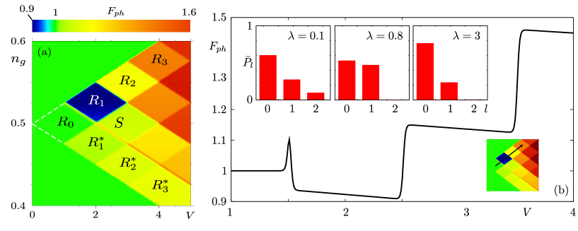
Figure 2: (a) Color map of the numerically calculated phonon Fano factor $F_{ph}$ as a function of $V$ (units $\omega_{0}/e$) and $n_{g}$ for $A=0.1$, $\lambda=0.8$, $k_{B}T=0.01\ \omega_{0}$, $\bar{U}=\ 20\ \omega_{0}$ and $\Gamma_{L}=10^{-3}\omega_{0}$. (b) Main: $F_{ph}$ as a function of $V$ (units $\omega_{0}/e$) calculated along the line $\bar{U}(1-2n_{g})+eV-\omega_{0}=0$ in the $V$, $n_{g}$ plane (corresponding to the black arrow in the bottom right scheme). Inset: phonon distributions $\bar{P}_{l}$ as a function of $l$ for different values of $\lambda$, calculated in the middle of region $R_{1}$ ($n_{g}=0.525$, $eV=3\omega_{0}$); other parameters as in (a). For $\lambda=0.1,0.8,3$ (left to right panels) it is $F_{ph}\approx 1.2,0.9,1.3$ respectively.

Fig. 2(a) shows a color map of the numerically calculated $F_{ph}$ as a function of $V$ and $n_{g}$ for ${\bar{U}}=20\,\omega_{0}$. It displays a checkerboard pattern where each region is characterized by the activation of transport channels involving transitions between different phonon states. The regions $R_{p}$ and $R_{p}^{*}$ will be particularly important for the following discussions. Their center is at

$$V^{(c)}=(p+1)\frac{\omega_{0}}{e}\quad\quad;\quad\quad n_{g}^{(c)}=\frac{1}{2}\pm\frac{\omega_{0}}{2\bar{U}}p$$ (32)

with the $+$ ($-$) sign for region $R_{p}$ ($R_{p}^{*}$). As stems from (22),(23) the following conditions are necessary for transitions to be open

$$|0,l+q\rangle \to |1,l^{\prime}+q\rangle\ \Leftrightarrow\ 2\omega_{0}(l^{\prime}-l)+\bar{U}(1-2n_{g})\pm eV\leq 0$$ (33)

$$|1,l+q\rangle \to |0,l^{\prime}+q\rangle\ \Leftrightarrow\ 2\omega_{0}(l^{\prime}-l)-\bar{U}(1-2n_{g})\pm eV\leq 0\,.$$ (34)

For the values of $V$ and $n_{g}$ within region $R_{p}$, it follows that the transitions (33) are open if $l^{\prime}\leq l+p$, while for the transitions (34) one needs $l^{\prime}\leq l$. Similarly, in regions $R_{p}^{*}$ one finds that for the transitions (33) one has $l^{\prime}\leq l$ while for (34) it is $l^{\prime}\leq l+p$.

Thus, in region $R_{0}$ the transition rates towards excited phonon states are all closed, therefore only the $l=0$ phonon state is populated. Here, the solution of the rate equations is simply given by $\bar{P}_{00}=A/(A+2)$, $\bar{P}_{10}=1-\bar{P}_{00}$ (for $T\ll\ \omega_{0}/k_{B}$) and one gets a super-Poissonian behavior

$$F_{ph}=1+\lambda\frac{2A}{2+A}\frac{(2n_{g}-1)^{2}}{(2+A)n_{g}^{2}-4n_{g}+2}>1\,.$$

The situation is more interesting in the other regions displayed in the figure. Indeed, in most of them the out of equilibrium phonon bath displays a super–Poissonian character. However, one can note that sub–Poissonian values, $F_{ph}<1$, are present at low voltages in region $R_{1}$ as shown also in the main panel of Fig. 2(b). Concentrating on $R_{1}$, the selective population arises if the following conditions are met:

($i$) the allowed phonon transitions $|n,l\rangle\to|n^{\prime},l^{\prime}\rangle$ must satisfy $l^{\prime}\leq 1+l$, which implies no direct population of the states with $l\geq 2$ from an initial state $|n,0\rangle$;

($ii$) the asymmetry has to be $A<1$, which suppresses the rate for tunnel–out transition $|1,l\rangle\to|0,l^{\prime}\rangle$ since for $V>0$ electrons flow from the left to the right lead.

Condition ($i$) is precisely realized in region $R_{1}$. By virtue of this, in order to populate excited phonon states with $l\geq 2$ starting from the phonon ground state $l=0$ within $R_{1}$, one needs to perform at least the following sequence of transitions

$$|0,0\rangle\to|1,1\rangle\to|0,1\rangle\to|1,2\rangle\to\ldots\,.$$ (35)

This implies that at least $l-1$ tunnel–out events are performed in $R_{1}$ in order to populate an excited state with $l\geq 1$ and this leads to $\bar{P}_{l\geq 1}\propto A^{l-1}$.

Condition ($ii$) and the above result induce a small occupation of the $l\geq 2$ states for $A<1$ [27]. The inset of Fig. 2(b) shows the phonon distribution in region $R_{1}$ for $A=0.1$ and three different coupling strengths. One can observe that all distributions are markedly out of equilibrium and very different from a thermal population, see the blue bar in Fig. 1(b). In addition, only the case of intermediate coupling $\lambda=0.8$ (second panel) displays a selective population as defined above. For small $\lambda$ (first panel) broad phonon distributions are obtained. On the other hand, for $\lambda>1$, the phonon distribution gets very narrow with $\bar{P}_{0}\gg\bar{P}_{l\geq 1}$ and no selective phonon population as in (31) may be achieved.

As a result of the competition between asymmetry, coupling strength and charge fluctuations, it is possible to find $F_{ph}<1$ only in the parameter space characterized by both $\lambda\lesssim 1$ and $A<A_{c}(\lambda)<1$ where $A_{c}(\lambda)$ is a threshold asymmetry of order unity for $\lambda\approx 1$ [27]. Furthermore, it is possible to show [27] that similar arguments apply in the region $S$ with a much stronger asymmetry, while region $R_{1}^{*}$ is similar to $R_{1}$, inverting the asymmetry: $A\to 1/A$.

In all other regions $R_{p\geq 2}$ and $R_{p\geq 2}^{*}$, the transitions $|n,l\rangle\to|n^{\prime},l^{\prime}\rangle$ with $l^{\prime}\leq l+p$ and $p\geq 2$ are active. Now, the transitions $|n,0\rangle\to|n^{\prime},l^{\prime}\rangle$ with $l^{\prime}\leq p$ directly populate phonon states with $l^{\prime}\geq 2$ from the phonon ground state $|n,0\rangle$. As a result, the mechanism to obtain a selective population discussed above is no longer effective, and broad phonon distributions are attained for $\lambda\lesssim 1$. They neither display a selective population, nor $F_{ph}<1$. Finally, for $\lambda>1$, narrow distributions arise and again no $F_{ph}<1$ is obtained.

3.2 Double occupancy

We now turn to analyze the effects of the dot double occupancy on the phonon distribution. We focus on the case of $\lambda\lesssim 1$ and $A<1$ which, as we discussed above, favors $F_{ph}<1$ when $\bar{U}$ is large. The choice $A<1$ is also favorable for obtaining double occupancy, as tunnel–out rates are suppressed. We will concentrate on the regime $\bar{U}>2\omega_{0}$ that is relevant in realistic situations with an intermediate dot–phonon coupling strength.

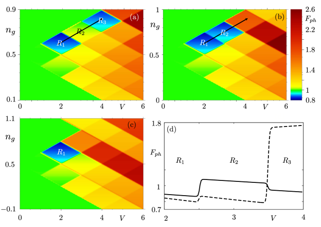
Figure 3: (a–c) Color map of the phonon Fano factor $F_{ph}$ in the $V$ (units $\omega_{0}/e$), $n_{g}$ plane for $A=0.1$, $\lambda=0.8$, $k_{B}T=0.01\ \omega_{0}$, $\Gamma_{L}=10^{-3}\omega_{0}$ and different values of $\bar{U}$: (a) $\bar{U}=5\ \omega_{0}$, (b) $\bar{U}=4\ \omega_{0}$, (c) $\bar{U}=3\ \omega_{0}$. (d) $F_{ph}$ as a function of $V$ (units $\omega_{0}/e$) calculated along the line $\bar{U}(1-2n_{g})+eV-\omega_{0}=0$ for $\bar{U}=5\ \omega_{0}$ (solid) and $\bar{U}=4\ \omega_{0}$ (dashed) (see the black arrows in panels (a), (b)).

Figs. 3(a)–(c) show $F_{ph}$ for the same parameters as in Fig. 2(a) but much smaller $\bar{U}$. In addition to region $R_{1}$, it is now $F_{ph}<1$ in region $R_{3}$ for $\bar{U}=5\ \omega_{0}$ and in region $R_{2}$ for $\bar{U}=4\ \omega_{0}$. A plot of $F_{ph}$ calculated along the diagonal line shown in Figs. 3(a) and 3(b) is displayed in panel (c). Note that the new regions where $F_{ph}<1$ shift at larger voltages with increasing $\bar{U}$. This explains why the case $\bar{U}\gg\omega_{0}$ is similar to the case $\bar{U}\to\infty$ near the resonance $n=0\to 1$, where only the region $R_{1}$ displays $F_{ph}<1$. The above behaviors represent special cases of the non–trivial general result: for obtaining $F_{ph}<1$ in region $R_{p\geq 2}$ it is necessary to have

$$(p+1)\omega_{0}<\bar{U}<(p+3)\omega_{0}\,.$$ (36)

In the following, we will explain the origin of Eq. (36) and show that it relates to specific transitions which involve the state $n=2$.

Let us first of all determine the conditions under which double occupancy can be achieved. In the absence of phonons ($\lambda=0$) the onset of the transition $n=1\to 2$ occurs for $V\geq V_{0}=U(3-2n_{g})/e$. On the other hand, in the presence of phonons, the state $|2,0\rangle$ can be occupied for smaller $V$: indeed, the transitions $|1,l+q\rangle\to|2,q\rangle$ with $l\geq 1$ are active for $V>V_{l}=[\bar{U}(3-2n_{g})-2l\omega_{0}]/e$, with $V_{l}<V_{0}$. This phonon–mediated mechanism for obtaining a double occupancy is similar to that described by Shen et al. [42] for the occupation of the LUMO in a molecular quantum dot. The condition for having the transition $|1,l+q\rangle\to|2,q\rangle$ open on the left barrier (forward transition, relevant for $V>0$) is

$$\bar{U}(1-2n_{g})-2\omega_{0}l+2\bar{U}-eV\leq 0\,.$$ (37)

In view of voltages constraints (32) for region $R_{p}$, the above transitions open there for $\bar{U}<(p+l+1)\omega_{0}$. We will now show that double occupancy can lead to a selective phonon population with $\bar{P}_{0}\approx\bar{P}_{1}\gg\bar{P}_{l\geq 2}$ in the regions $R_{p\geq 2}$. For $\bar{U}<(p+3)\omega_{0}$ the transitions

$$|1,l+q\rangle\to|2,q\rangle\quad\quad l\geq 2$$ (38)

are active within $R_{p}$ and decrease the occupation probability of the excited phonon bath states with $l\geq 2$. They come in addition to the usual transitions

$$|1,l\rangle\to|0,l^{\prime}\rangle\quad\quad l^{\prime}<l$$ (39)

which also depopulate the excited phonon states and were already present when $\bar{U}\gg\omega_{0}$. Note that these latter transitions alone are not sufficient to give rise to a selective phonon population: indeed, broad phonon distributions are obtained for $\lambda<1$ in $R_{p\geq 2}$ as already discussed in Sec. 3.1. Now, since for $A<1$ and $V>0$ tunnel–in events are faster than tunnel–out ones, the new transitions (38), are much more effective than transitions (39) in depopulating states with $l\geq 2$. With these new fast channels it is now possible to obtain lower occupations of all the excited phonon bath states up to $l=2$, eventually leading to a selective phonon population.

This explains the right hand side of the inequality (36). To obtain the left hand side of (36) it is sufficient to recognize that if $\bar{U}<(p+1)\omega_{0}$ the additional depopulation transitions $|1,l+q\rangle\to|2,q\rangle$ with $l\geq 1$ are open in all $R_{p}$. They also deplete the states with $l=1$, eventually leading to too a narrow distribution with $\bar{P}_{0}\approx 1$ and $F_{ph}>1$.

Therefore, tuning $\bar{U}$ it is possible to trim the shape of phonon population from broad, to selective, up to a very narrow distribution.

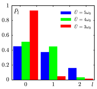
Figure 4: Phonon distribution $\bar{P}_{l}$ as a function of $l$ calculated in the center of region $R_{2}$ for different values of $\bar{U}$, all other parameters as in Fig. 2(a). For $\bar{U}=5\omega_{0},4\omega_{0},3\omega_{0}$ it is $F_{ph}\approx 1.1,0.8,1.5$, respectively.

Figure 4 shows $\bar{P}_{l}$ as a function of $l$, calculated in the center of $R_{2}$ for different $\bar{U}$, all other parameters are the same as in Fig. 2(a). For $\bar{U}=5\omega_{0}$, the transitions $|1,2+q\rangle\to|2,q\rangle$ are closed and a broad phonon distribution (blue bars) with $F_{ph}>1$ is obtained. When $\bar{U}=4\ \omega_{0}$, the above transitions are open and the channel $|1,2\rangle\to|2,0\rangle$ creates the selective population displayed by the green bars. Further reducing $\bar{U}=3\ \omega_{0}$, also the transitions $|1,1\rangle\to|2,0\rangle$ opens up and the resulting narrow distribution displays super–Poissonian character.

4 Damping effects and the validity of the RWA

In Section 2.3 we have discussed the out of equilibrium localized bath arising in the transport regime, concentrating particularly on the occurrence of sub–Poissonian phonon distributions. The results were derived assuming that the localized phonon mode has an infinite life time in the absence of tunneling. In addition, up to now we have always considered the case of a fast motion of the oscillator in comparison to the transport time scales and adopted the RWA. In this section we study the robustness of the results, when the above conditions are relaxed.

4.1 Towards a relaxed single mode bath

In order to damp the single mode bath towards an equilibrium distribution, we couple it to a conventional dissipative environment, represented by a set of harmonic oscillators

$$H_{b}^{(3)}=\sum_{j}\omega_{j}b^{\dagger}_{j}b_{j}$$ (40)

with a linear coupling

$$H_{bb}^{(13)}=(b+b^{\dagger})\sum_{j}\chi_{j}\omega_{j}(b_{j}+b^{\dagger}_{j})$$ (41)

and bath spectral density $J(\omega)=2\pi\sum_{j}\omega^{2}_{j}\chi_{j}^{2}\delta(\omega-\omega_{j})$. In the presence of the additional bath (40), it is still possible to diagonalize exactly $H_{\lambda}$ by means of a canonical transformation which also involves the operators $b_{j}$, $b_{j}^{\dagger}$ [12, 20]. Following a derivation analogous to that discussed in Sec. 2.2 and treating both Eq. (9) and Eq. (41) to the lowest perturbative order, we obtain the following stationary rate equations in the RWA [42, 20]

$$-z_{n}\bar{P}_{nq}\sum_{k=\pm 1\atop 0\leq n+k\leq 2}\sum_{p=0}^{\infty}\Gamma_{qp}^{n,n+k}+\sum_{k=\pm 1\atop 0\leq n+k\leq 2}\sum_{p=0}^{\infty}z_{n+k}\bar{P}_{n+k,p}\Gamma^{n+k,n}_{pq}$$

$$+\sum_{p=0}^{\infty}\bar{P}_{np}\Gamma^{rel}_{pq}-\sum_{p=0}^{\infty}\bar{P}_{nq}\Gamma^{rel}_{qp}=0\,.$$ (42)

The relaxation rates

$$\Gamma^{rel}_{q,q-1}=e^{\beta\omega_{0}}\Gamma^{rel}_{q-1,q}=qw\Gamma_{L}{\left(1-e^{-\beta\omega_{0}}\right)}^{-1}$$ (43)

induce transitions $|n,q\rangle\to|n,q\pm 1\rangle$ and drive the single mode bath towards thermal equilibrium, while the tunneling rates $\Gamma_{pq}^{nn^{\prime}}$ are those described in Sec. 2.3. Here, $w=J(\omega_{0})/\Gamma_{L}$ parametrizes the relaxation strength. For $w\to\infty$, phonons are completely relaxed and $\bar{P}_{l}\to\bar{P}_{l}^{(th)}$, characterized by a super–Poissonian Fano factor.

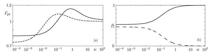
Figure 5: (a) Phonon Fano factor $F_{ph}$ for $A=0.1$ (solid) and $A=0.01$ (dashed) as a function of the relaxation strength $w$ (log scale) for $\bar{U}=4\ \omega_{0}$, $eV=3\ \omega_{0}$ and $n_{g}=0.75$ (the center of $R_{2}$). All other parameters as in Figs. 3(a)–(c). (b) Phonon populations $\bar{P}_{0}$ (solid), $\bar{P}_{1}$ (dashed) as a function of $w$ (log scale) for the same parameters as in (a).

The effects of relaxation on the phonon distribution are illustrated in region $R_{2}$ for $\bar{U}=4\ \omega_{0}$. All other regions display qualitatively similar behavior. Fig. 5(a) shows $F_{ph}$ as a function of $w$, calculated in the center of $R_{2}$. As $w$ increases, $F_{ph}$ crosses from $F_{ph}<1$ in the unequilibrated regime to a super–Poissonian maximum, before reaching the thermal value which, for $T\ll\omega_{0}/k_{B}$, is only slightly above 1. The effects of relaxation become relevant when the typical life time of the excited phonon bath $\tau_{rel}=J(\omega_{0})^{-1}$ is comparable with the slowest typical charge dwell time $\tau_{tr}=(\mathrm{min}\{1,A\}\Gamma_{L}e^{-\lambda})^{-1}$. This explains also the shift of the maximum towards smaller $w$ for smaller asymmetries observed in Fig. 5(a). In Fig. 5(b), one can see that for increasing relaxation, the selective phonon population is destroyed with a tendency towards an almost full occupation of the $l=0$ state, in accordance with a low temperature $\bar{P}_{l}^{(th)}$ (see Eq. (25).

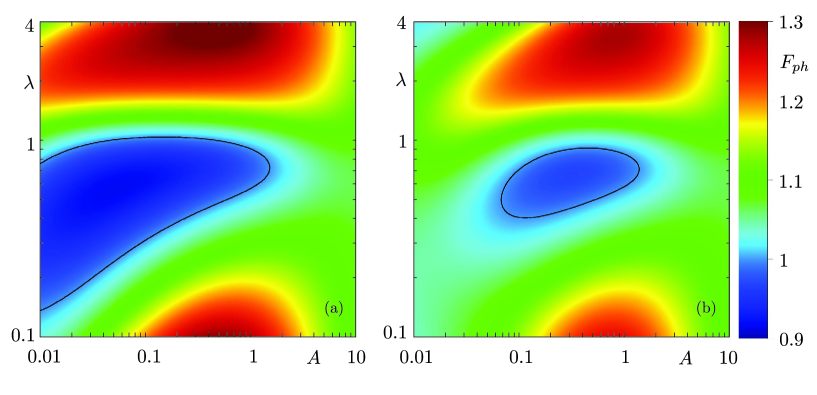
Figure 6: (a) Color map of $F_{ph}$ as a function of $A$, $\lambda$ (both in log scale), for $eV=2\ \omega_{0}$, $n_{g}=0.625$ (region $R_{1}$), $\bar{U}=4\ \omega_{0}$ and $w=0.01$, other parameters as in Figs. 3(a)–(c). The black contour line is set at $F_{ph}=1$. (b) Same as panel (a) but with $w=0.1$.

We now analyze the robustness of the sub–Poissonian phonon bath against $w$ varying the parameters $A$, $\lambda$. Figures 6(a) and 6(b) show a color map of $F_{ph}$ as a function of $A$ and $\lambda$ in the middle of the region $R_{1}$ for two different values of the relaxation strength. Superimposed to the color map, the black contour line signals $F_{ph}=1$. This line corresponds to the “stability boundary” of the sub–Poissonian phonon distribution with respect to asymmetry and coupling strength. Increasing relaxation, Fig. 6(b), the region of $A$ and $\lambda$ where $F_{ph}<1$ shrinks, the regime $A\ll 1$ is more strongly affected, in accordance with the discussion above, while the sub-Poissonian distribution is still stable for not too small $A<1$ and $\lambda\approx 1$. Qualitatively analogous results are observed in every region $R_{p}$.

4.2 Validity of the RWA

When the dynamics of the single mode bath is not much faster than the typical electron tunneling rate the RWA is no longer justified and the fully coherent GME in Eq. (18) must be solved. In this case, also the non diagonal elements of the density matrix will be different from zero in the stationary regime. Even more important, while in the RWA the diagonal elements $\bar{\rho}_{ll}^{n}$ of the density matrix are decoupled from the off–diagonal ones, in general this is no longer the case. Thus the coherences $\bar{\rho}_{l,l^{\prime}\neq l}$ may influence the phonon distribution $\bar{P}_{nl}$. In this last part, we will present preliminary results showing this effect. For simplicity, we consider $\bar{U}\gg\omega_{0}$, without relaxation $w=0$.

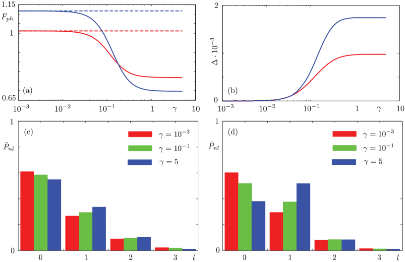
Figure 7: (a) Solid: phonon Fano factor $F_{ph}$ obtained from the solution of Eq. (18) as a function of $\gamma=\Gamma_{L}/\omega_{0}$ for $A=0.01$, $\lambda=0.1$, $T=0.1\ \omega_{0}/k_{B}$, $\bar{U}=20\ \omega_{0}$, and $eV=2\ \omega_{0}$ with $n_{g}=0.525$ (red, in region $R_{1}$) or $eV=3\ \omega_{0}$ with $n_{g}=0.5$ (blue, in region $S$). Dashed: $F_{ph}$ obtained from the RWA. (b) Relative difference $\Delta$ between $F_{ph}$ and $F_{ph}^{0}$ (see text for definition), as a function of $\gamma$ for the same parameters as panel (a). (c) Diagonal elements $\bar{P}_{l}$ of the solution of Eq. 18 as a function of $l$ calculated for $eV=2\ \omega_{0}$ and $n_{g}=0.525$ and different values of $\gamma$. (d) Same as (c) but for $eV=3\ \omega_{0}$ and $n_{g}=0.5$.

Fig. 7(a) shows $F_{ph}$ obtained from the solutions of the full GME in Eq. (18) as a function of $\gamma=\Gamma_{L}/\omega_{0}$, where we keep $\omega_{0}$ fixed (note that the calculation of $F_{ph}$ via Eqs. (26) and (27) contains also averages of non–diagonal operators). The red curve corresponds to $F_{ph}$ in the center of region $R_{1}$, while the blue one gives $F_{ph}$ in region $S$. The dashed lines correspond to the RWA solution. In both cases, it is clear that deviations from the RWA (dashed line) occur for $\gamma>0.05$. For increasing values of $\gamma$, $F_{ph}$ saturates into a new regime, characterized by sharply reduced phonon fluctuations.

In order to assess the relevance of the off–diagonal density matrix elements, we have evaluated the ratio $\Delta=|F_{ph}-F^{0}_{ph}|/F_{ph}$, where $F_{ph}^{0}$ is calculated from the GME solution neglecting the coherences $\bar{\rho}_{l,l^{\prime}\neq l}^{n}$. We show $\Delta$ in Fig. 7(b): clearly, the impact of the off–diagonal terms on $F_{ph}$ is very small, with $\Delta<2\cdot 10^{-3}$. This fact is supported also by direct inspection of the largest $\bar{\rho}_{l,l^{\prime}\neq l}^{n}$, whose absolute values are three to four orders of magnitude smaller than the leading diagonal terms. The origin of the reduction of $F_{ph}$ in Fig. 7a therefore lies in a modification of $\bar{P}_{nl}$, mediated by the off–diagonal terms of the density matrix.

In Fig. 7 we show the population of the phonon bath $\bar{P}_{l}$ obtained in $R_{1}$, panel (c), and in $S$, panel (d). The changes mentioned above can be clearly seen: in $R_{1}$, for increasing $\gamma$ the phonon population gets broader. In $S$ an inversion of the population for the levels $l=0$ and $l=1$ is present, with an even stronger sub–Poissonian $F_{ph}$.

The preliminary results show that there are regimes where dynamical coherent effects are relevant for the single phonon distribution. Much in the same way as for $\bar{U}$, phonon distributions can be dramatically shaped by tuning $\gamma$. Strictly speaking, the results for $\gamma>0.1$ and $k_{B}T=0.1\omega_{0}$ imply $\Gamma_{L}>k_{B}T$ and therefore fall beyond the limits of the sequential tunneling regime for the calculation presented above. In this case we can expect that the additional coherent dot dynamics could lead to even larger deviations with respect to the RWA solutions.

5 Conclusions

In this paper we have analyzed the out of equilibrium properties of an unconventional single mode phonon bath, coupled to a quantum dot, in terms of its phonon distribution and the respective Fano factor. We have described the combined evolution of the dot and the bath degrees of freedom by means of a GME. In the regime of validity of the RWA, corresponding to a fast bath motion, we have shown that the out of equilibrium phonon bath markedly differs from a thermal one. The transport properties of the dot in the presence of a thermal or an unequilibrated single bath mode are qualitatively different. In the case of a single occupancy of the quantum dot, we have identified the transport regimes and the range of asymmetries $A$ and dot–bath coupling strengths $\lambda$ for which a sub–Poissonian phonon distribution appears. We have interpreted such distribution in terms of a peculiar, selective population of the bath modes. Double occupancy of the dot may act as a filter on the phonon bath distribution, eventually turning $F_{ph}<1$ in regions where a super–Poissonian distribution would be attained in the case of a single dot occupancy. The crossover from an unequilibrated phonon bath to a thermal regime has been investigated by coupling the single bath mode to an external dissipative environment. For increasing damping strength, the sub–Poissonian phonon bath is destroyed and the latter tends to a thermal one. The crossover from a sub– to super–Poissonian bath has been analyzed as a function of $A$ and $\lambda$. We have found that $F_{ph}<1$ survives up to relatively strong damping when $A\approx 1$ and $\lambda\approx 1$. Finally, we have shown that in the case of $\omega_{0}$ not much larger than the tunneling rates, the RWA is no longer valid and the solutions of the full GME display strong modifications when the coherent dynamics of the bath is fully taken into account. In particular, we have shown that although off–diagonal density matrix elements remain small in the coherent regime, their coupling to the diagonal elements gives rise to significant modifications of the latter. These results show that by suitably tuning the quantum dot properties, it is possible to obtain a variety of unconventional single phonon baths characterized by a wide range of phonon distributions. A detailed analysis of the coherent regime and the possible extension to out of equilibrium baths with two or few more phonon modes is deferred to future work.

6 Acknowledgements

The authors acknowledge stimulating discussions with F. Haupt, M. Merlo and A. Braggio. Financial support by the EU via contract no. MCRTN-CT2003-504574 and by the Italian MIUR via PRIN05 is gratefully acknowledged.

References

References

- [1] Caldeira A O and Leggett A J 1983 Ann. Phys. 149 374
- [2] Leggett A J, Chakravarty S, Dorsey A T, Fisher Matthew P A, Garg Anupam and Zwerger W 1987 Rev. Mod. Phys. 59 1
- [3] Weiss U 1999 Quantum dissipative systems (World Scientific, Singapore)
- [4] Duty T, Gunnarsson D, Bladh K, and Delsing P 2004 Phys. Rev. B 69, 140503(R)
- [5] Simmonds R W, Lang K M, Hite D A, Nam S, Pappas D P and Martinis J M 2004 Phys. Rev. Lett. 93 077003; Lisenfeld J, Lukashenko A, Ansmann M, Martinis J M and Ustinov A V, 2007 Phys. Rev. Lett. 99 170504
- [6] Paladino E, Faoro L, Falci G and Fazio R, 2002 Phys. Rev. Lett. 88 228304; Galperin Y M, Altshuler B L, Bergli J and Shantsev D V 2006 Phys. Rev. Lett. 96 097009; Paladino E, Sassetti M, Falci G, Weiss U 2008 Phys. Rev. B, 77 041303(R)
- [7] Wallraff A, Schuster D I, Blais A, Frunzio L, Huang R -S, Majer J, Kumar S, Girvin S M and Schoelkopf R J 2004 Nature 431 162
- [8] Nesi F, Grifoni M and Paladino E 2007 New J. Phys. 9 316
- [9] Debald S, Brandes T and Kramer B 2002 Phys. Rev. B 66 041301(R)
- [10] Weig E M, Blick R H, Brandes T, Kirschbaum J, Wegscheider W, Bichler M and Kotthaus J P 2004 Phys. Rev. Lett. 92 046804
- [11] Park H, Park J, Lim Andrew K L, Anderson E H, Alivisatos A P and McEuen P L 2000 Nature 407 57
- [12] Braig S and Flensberg K 2003 Phys. Rev B 68 205324
- [13] Sapmaz S, Jarillo–Herrero P, Blanter Ya M, Dekker C and van der Zant H S J 2006 Phys. Rev. Lett. 96 026801
- [14] LeRoy B J, Lemay S G, Kong J and Dekker C 2004 Nature 432 371
- [15] Boese D and Schoeller H 2001 Europhys. Lett. 54 668
- [16] Zazunov A, Feinberg D and Martin T 2006 Phys. Rev. B 73 115405
- [17] Naik A, Buu O, LaHaye M D, Armour A D, Clerk A A, Blencowe M P and Schwab K C 2006 Nature 443 193
- [18] Mitra A, Aleiner I and Millis A J 2004 Phys. Rev B 69 245302
- [19] Koch J, von Oppen F and Andreev A V 2006 Phys. Rev. B 74 205438
- [20] Haupt F, Cavaliere F, Fazio R and Sassetti M 2006 Phys. Rev. B 74 205328; Haupt F, Cavaliere F, Fazio R and Sassetti M 2008 Physica E 40 1267
- [21] Lüffe M C, Koch J and von Oppen F 2008 Phys. Rev. B 77 125306
- [22] Rodrigues D A and Armour A D 2005 New. J. Phys. 7 251
- [23] Rodrigues D A, Imbers J and Armour A D 2007 Phys. Rev. Lett. 98 067204
- [24] Koch J, Semmelhack M, Von Oppen F, and Nitzan A 2006 Phys. Rev. B 73, 155306
- [25] Wegewijs M and Nowack K C 2005 New J. Phys. 7 237
- [26] Takas S, Kim Y B and Mitra A 2005 Phys. Rev. B 72 075337
- [27] Merlo M, Haupt F, Cavaliere F and Sassetti M 2008 New J. Phys. 10 023008
- [28] Loudon R 2000 The quantum theory of light (3rd edition, Oxford University Press, Oxford)
- [29] Kimble H J, Dagenais M and Mandel L 1977 Phys. Rev. Lett. 39 691
- [30] Itano W M, Bergquist J C and Wineland D J 1988 Phys. Rev. A 38 559
- [31] König J, Schoeller H and Schön G 1996 Phys. Rev. B 54 16820
- [32] Knobel R G and Cleland A N 2003 Nature 424 291
- [33] Armour A D, Blencowe M P and Zhang Y 2004 Phys. Rev. B 69 125313
- [34] Koch J, Sela E, Oreg Y and von Oppen F 2007 Phys. Rev. B 75 195402
- [35] Cornaglia P S, Ness H and Grempel D R 2004 Phys. Rev. Lett. 93 147201
- [36] Mravlje J, Ramšak A and Rejec T 2005 Phys. Rev. B 72 121403(R)
- [37] Cohen-Tannoudji C, Dupont-Roc J and Grynberg G 1993 Atom-Photon Interactions (Wiley–Interscience)
- [38] Sassetti M and Weiss U 1994 Europhys. Lett. 27 311
- [39] Cavaliere F, Braggio A, Stockburger J T, Sassetti M and Kramer B 2004 Phys. Rev. Lett. 93 036803; Cavaliere F, Braggio A, Sassetti M and Kramer B 2004 Phys. Rev. B 70 125323
- [40] Shnirman A and Schön G 1998 Phys. Rev. B 57 15400
- [41] Mandel L and Wolf E 1995 Optical Coherence and Quantum Optics (New York: Cambridge University Press)
- [42] Shen X Y, Dong B, Lei X L and Horing N J M 2007 Phys. Rev B 76 115308