Detecting Sound-Wave-Like Surface Brightness Ripples in Cluster Cores

Abstract

We investigate the observational requirements for the detection of sound-wave-like features in galaxy cluster cores. We calculate the effect of projection on the observed wave amplitude, and find that the projection factor depends only weakly on the underlying cluster properties but strongly on the wavelength of the sound waves, with the observed amplitude being reduced by a factor $\sim 5$ for $5{\rm\thinspace kpc}$ waves but only by a factor $\sim 2$ for $25{\rm\thinspace kpc}$ waves. We go on to estimate the time needed to detect ripples similar to those previously detected in the Perseus cluster in other clusters. We find that the detection time scales most strongly with the flux of the cluster and the amplitude of the ripples. By connecting the ripple amplitude to the heating power in the system, we estimate detection times for a selection of local clusters and find that several may have ripples detected with $\sim 1{\rm\thinspace Ms}$ Chandra time.

1 Introduction

The thermal history of the hot gas in galaxy clusters has been a long-standing puzzle to astronomers. In many clusters (often referred to as cool-core clusters), the cooling time of the hot X-ray emitting IntraCluster Medium (ICM) drops to a fraction of the age of the universe in the brightest central regions. The first models of these clusters suggested that a significant amount of the gas should form a “cooling flow”, in which gas in the cluster core cools out of the X-ray band, reducing the pressure support on the surrounding material and causing the outer gas to flow toward the centre. The cool gas predicted by this model is expected to fuel star formation in the brightest cluster galaxy. However, it has long been known that the star formation rates in these systems are significantly lower than these cooling flow models would predict.

With the launch of the most recent generation of X-ray satellites — particularly Chandra and XMM-Newton — it has been shown that the amount of cool X-ray emitting gas in clusters is much smaller than predicted by the simple cooling flow models (Peterson et al., 2003). This has led to the widely accepted conclusion that the ICM is being heated, reducing the cooling flow to around $10$ percent of the expected value (see e.g. Peterson & Fabian 2006 or McNamara & Nulsen 2007 for reviews).

At the same time that Chandra and XMM-Newton have confirmed that heating of cluster cores is required, there have been substantial advances in identifying possible heating mechanisms. Whilst there are a large number of possible heating mechanisms, the current leading contender is mechanical energy injection by the central black hole. Evidence of the interaction between the ICM and the central cluster was first noted in ROSAT observations of the Perseus cluster (Böhringer et al., 1993), with relativistic plasma from the AGN jets displacing the ICM to form radio-emitting cavities. Since that time, detection of such cavities in nearby clusters has become commonplace, with a recent study by Dunn & Fabian (2006) showing evidence for X-ray cavities in at least $70$ percent of the clusters in their sample with short central cooling times and central temperature drops. The work done on the ICM in the inflation of these cavities provides a plausible source for the heating of the ICM, and several studies have shown that the power associated with the bubbles’ inflation is sufficient to offset the cooling luminosity (Bîrzan et al., 2004; Dunn & Fabian, 2004; Rafferty et al., 2006; Dunn et al., 2005).

Despite the promise shown by the AGN-injection model of cluster-core heating, there are a substantial number of details that remain unclear. One particular problem is how the energy injected by the AGN near the cluster core is distributed over the whole cooling region in a quasi-isotropic manner. The peaked central metal abundances in many cool-core clusters indicate that this process must be gentle, suggesting that it is not simply a matter of clusters having occasional unusually large outbursts that heat the outer regions.

A possible clue to the method of energy transport away from the cluster core was given by the unexpected detection of quasi-spherical ripples in the surface brightness structure in the Perseus cluster (Fabian et al., 2003), shown in Fig. 1 with a high pass filter applied to remove the underlying cluster emission (reproduced from Sanders & Fabian 2007). Ripples in surface brightness are indicative of fluctuations in the density of the ICM and consequentially, these features have been interpreted as sound waves generated by the cavity inflation process. Such sound waves are expected to be effective in distributing the AGN’s mechanical energy input over the entire cluster core (McNamara & Nulsen, 2007) and, in the case of Perseus, it has been shown that the energy they carry is comparable to that required to offset the cooling Sanders & Fabian (2007).

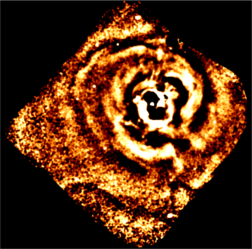
Figure 1: A $900{\rm\thinspace ks}$ Chandra image of the Perseus cluster core, with a high pass filter applied to remove the underlying surface brightness profile and show the ripples. It is clear that the ripples are highly symmetric about the central source, but not coherent over the full $2\pi$. Reproduced from Sanders & Fabian (2007)

Whilst cavities are common, associated sound waves have never been detected in a cluster other than Perseus. However, the Perseus cluster is both a factor of $\sim 2$ brighter than any other cluster and has a factor $2$ more observation time than any other cluster. In order to understand whether sound waves do indeed play a general role in the heating of cluster cores, however, their presence needs to be confirmed in other systems. Our main aim in this paper is to investigate the relationship between the intrinsic and observed properties of sound waves in galaxy clusters and to assess the prospects for detecting sound waves in systems other than Perseus. To do this, we will not try to model the detailed time evolution of ripples in cluster cores, but will assume that the almost-monochromatic, low amplitude, ripples in Perseus are a good template for the features expected in other clusters. By imposing ripples derived from this template on model clusters, we will determine how the detection time varies with the properties of the ripples and the underlying cluster profile.

Throughout the paper we adopt a cosmology where $H_{0}=70{\rm\thinspace km}{\rm\thinspace s}^{-1}{\rm\thinspace kpc}^{-1}$, $\Omega_{M}=0.3$ and $\Omega_{\Lambda}=0.7$. The redshift of the Perseus cluster is 0.018.

2 Effect of projection on ripple amplitudes

Inferring information about extended sources such as galaxy clusters is complicated by the fact that, whilst the source is intrinsically three dimensional, our view of it is only two dimensional. In the case of an idealised spherically symmetric cluster, the image as viewed on the sky is related to the underlying emission profile by the Abel integral:

$$I(b)=\int^{\infty}_{b}\frac{2r\epsilon(r)}{\sqrt{r^{2}-b^{2}}},$$ (1)

where $b$ is the projected distance on the sky, $r$ is the 3-dimensional radius, $\epsilon$ is emissivity and $I$ is the surface brightness.

Ignoring the effect of projection, a monochromatic density wave in an isothermal galaxy cluster with $\epsilon\propto n^{2}_{e}$ will lead to an emissivity profile of the form

$$\epsilon\propto\left(\left[1+f\sin\left(\frac{2\pi}{\lambda}r\right)\right]n\right)^{2},$$ (2)

where $f$ is the fractional amplitude of the density wave. The corresponding amplitude of the emissivity fluctuations is then

$$h_{\epsilon}=\frac{\left(\left[1+f\sin\left(\frac{2\pi}{\lambda}r\right)\right]n\right)^{2}-n^{2}}{n^{2}}$$ (3)

$$=f^{2}\sin^{2}\left(\frac{2\pi}{\lambda}r\right)-2f\sin\left(\frac{2\pi}{\lambda}r\right)$$ (4)

i.e. the amplitude of the ripples in emissivity is $|h_{\epsilon}|\sim 2f$.

However, as noted by Fabian et al. (2006), the effect of projection is to reduce the magnitude of the surface brightness ripples so that in general $|h_{sb}|<|h_{\epsilon}|$, with troughs in the emissivity being filled by the surrounding peaks, and vice-versa. For the case of the Perseus cluster, (Fabian et al., 2006) found that projection acts such that $|h_{sb}|\sim f/2.5\sim|h_{\epsilon}|/5$. However this result is not universal as the extent to which a trough in emissivity is filled by the surrounding peaks depends on the relative overlap and emission of the peaks and troughs along the line of sight. This is a function both of the underlying surface brightness profile and the properties of the ripples themselves.

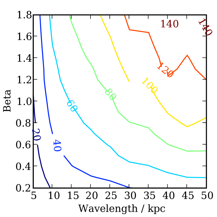
Figure 2: Amplitude of surface brightness ripple height as a percentage of the density ripple amplitude for a range of underlying density model $\beta$ parameters and density perturbation wavelengths and with fixed amplitude density perturbation $f=0.15$ and fixed density model $r_{\text{core}}=25{\rm\thinspace kpc}$.

To quantify the relationship between the wavelength and cluster properties and the projected ripple height, we have numerically calculated the projected ripple height for monochromatic ripples in clusters with an underlying beta-model density distribution (Cavaliere & Fusco-Femiano, 1976):

$$n_{e}=\frac{n_{e,0}}{\left(1+\left(r/r_{\text{c}}\right)^{2}\right)^{3\beta/2}},$$ (5)

where $r_{\text{c}}$ is the core radius of the cluster, $\beta$ is the beta parameter and $n_{e,0}$ is a normalisation. The beta model provides a reasonable fit to the density distribution in many clusters except in the innermost region where adding a second beta-model component often provides a better fit.

Fig 2 shows the median projected ripple height calculated for a isothermal $kT=6{\rm\thinspace keV}$ cluster with an underlying beta-model density distribution,

$$\frac{n_{e}}{{\rm\thinspace cm}^{-3}}=\frac{4.5\times 10^{-2}}{\left(1+\left(r/25{\rm\thinspace kpc}\right)^{2}\right)^{3\beta/2}},$$ (6)

with values of $\beta$ in the range $0.2-1.8$ and monochromatic density perturbations with $f=0.15$ and wavelengths in the range $5-50{\rm\thinspace kpc}$. The use of the median height reflects the fact that not all ripples have exactly the same height in projection, however the heights are consistent enough that the exact method of quantifying $|h_{sb}|$ for a given set of parameters does not significantly affect the results. The projected height decreases with shorter ripple wavelengths and shallower density profiles, which is expected as these are the conditions in which adjacent peaks and troughs in emissivity will have the most similar amplitude along the line of sight. Fig. 3 shows the projected height for a similar cluster but with $\beta=0.6$ and a range of core-radii. It is apparent that the amplitude of the surface brightness ripples is not a strong function of the core radius, although larger core radii — flatter emissivity profiles — do tend to show smaller surface brightness ripples, as expected.

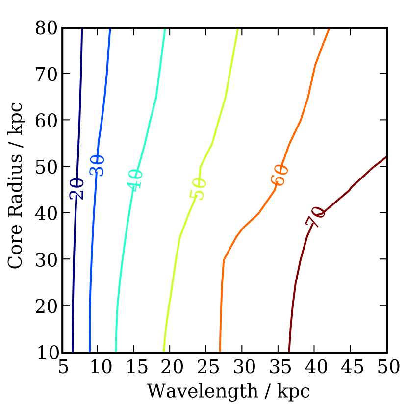
Figure 3: Amplitude of the surface brightness ripples as a percentage of the density ripple amplitude for a range of ripple wavelengths and beta-model core radii for fixed amplitude density perturbation $f=0.15$ and fixed $\beta=0.6$. The amplitude is almost independent of core radius for wavelengths below $25{\rm\thinspace kpc}$.

Testing clusters with fixed $\beta$ and core radius, but varying density amplitude, shows a linear variation in the projected amplitude over the entire range of density amplitudes likely to be relevant in clusters. This means that our calculations for a single ripple amplitude scale in a simple way to all amplitudes.

3 Time to Detect Ripples in Clusters

3.1 A Naive Approach

The basic condition to detect a ripple is that the variation in the number of counts in the peaks and troughs of the surface brightness profile are distinguishable from variations due purely to noise. Assuming a regime where Poisson noise dominates, this implies that to detect a single peak we require an observing time such that:

$$(n_{\text{ripple}}-n_{\text{no ripple}})t>\sigma\sqrt{n_{\text{no ripple}}t}$$ (7)

where $n_{\text{ripple}}$ is the average count rate in the ripple peak, $n_{\text{no ripple}}$ is the average count rate that would be observed in the peak without a ripple, $t$ is the time to detect the ripple, and $\sigma$ is the number of standard deviations above the mean we require for a detection. Therefore

$$t>\frac{\sigma^{2}n_{\text{no ripple}}}{(n_{\text{ripple}}-n_{\text{no ripple}})^{2}}.$$ (8)

Taking the underlying density profile to be a beta model and the cluster to be isothermal, the surface brightness profile will be a projected beta model, of the form (Ettori, 2000):

$$S(r)=S_{0}\left(1+\left(r/r_{\text{c}}\right)^{2}\right)^{0.5-3\beta}.$$ (9)

If the cluster is perfectly spherically symmetric and ripples are sinusoidal with a wavelength $\lambda$ and constant fractional surface brightness amplitude $h$ the detection time is:

$$t>\frac{\sigma^{2}}{2\pi S_{0}}\left(\int_{r_{0}}^{r_{0}+\lambda/2}r\Phi(r){\rm d}r\right)\\ \Bigg{(}\int_{r_{0}}^{r_{0}+\lambda/2}r\left(1+f\sin\left(\frac{2\pi r}{\lambda}\right)\right)\Phi(r){\rm d}r-\\ \int_{r_{0}}^{r_{0}+\lambda/2}r\Phi(r){\rm d}r\Bigg{)}^{-1}$$ (10)

where

$$\Phi(r)=\left(1+(\frac{r}{r_{\text{c}}})^{2}\right)^{0.5-3\beta},$$ (11)

and $S(r)=S_{0}\Phi(r)$ represents the projected surface brightness in counts per second per unit area at radius $r$. $r_{0}$, the lower limit of integration, is an integer number of wavelengths from the centre so the surface brightness is integrated over a peak. Taking some parameters appropriate for a Perseus-like cluster at $z\sim 0.018$; $\beta=0.5$, $r_{\text{c}}=30{\rm\thinspace kpc}$, $\lambda=15{\rm\thinspace kpc}$, $h=0.05$, $S_{0}=5{\rm\thinspace counts\thinspace s^{-1}\thinspace arcmin^{-2}}$ and $\sigma=3$, we find $t_{\text{detect}}=1.5{\rm\thinspace ks}$. This is clearly short compared to the time actually required to detect the sound waves in Perseus, which were not observed in a $25{\rm\thinspace ks}$ observation but were observed in a $200{\rm\thinspace ks}$ observation. Part of this discrepancy can be explained by the fact that our calculation assumes that the ripples are coherent over a entire annulus of the cluster. In practice, the ripples in Perseus are coherent over a much smaller angle. To detect a ripple over some fraction $\chi$ of an angle requires that the integration time is increased by a corresponding factor of $1/\chi$.

Although this method is simple and easy to apply, the assumption of a uniform monochromatic wave may lead to misleadingly small detection times. For this reason, we have developed a method for estimating the detection time numerically for a more general waveform.

3.2 An Improved Approach

To better constrain the time required for detection of ripples in distant clusters, we have developed a simple algorithmic approach to determining whether a cluster profile contains ripples. The input to the algorithm is a count rate profile either obtained from data or, for our purposes in the current work, generated artificially according to a method that will be described below. By generating artificial count rate profiles, we will be able to determine how the detection time for the ripples depends both on properties of the underlying cluster atmosphere and properties of the ripples themselves.

The algorithm we use to determine whether a cluster has detectable ripples is:

• Obtain a count rate profile $R$, either from data or from a model

• Optionally (for simulated profiles) add Poisson noise to the count rate (assuming the input profile is an average count rate)

• Convert the count rate profile to a surface brightness profile using the area of each annulus in the profile, to give an actual surface brightness profile $S$.

• Fit a projected beta model to the surface brightness profile to give an underlying surface brightness profile $B$.

• Calculate the fractional residuals of the actual surface brightness profile compared to the input surface brightness profile $a=(S-B)/B$

• Fit a 1D smoothing spline to the surface brightness residuals $a$ to give a smooth profile $a_{s}$. The degree of smoothing of the spline was adjusted by eye to provide an acceptable compromise between over-smoothing the ripples and closely following the noise in $S$.

• Use the zero points of $a_{s}$ to delimit peaks and troughs in the ripple.

• For each peak or trough determine the significance of the excess or deficit in count rate in that region in the actual count rate $R$ compared to the count rate that would result from the underlying surface brightness profile $B$.

• Retain peaks or troughs only if their significance is greater than some threshold $\sigma$; typically $\sigma=3$, is chosen.

At the end of this process, we have a list of radii that mark the end-points of regions containing significant excesses or decrements in emission. However such regions do not necessarily constitute ripples. In order that we see a region as a ripple there must be some adjacent regions of positive or negative excess emission. The effect of varying the number of adjacent regions required to constitute a detection is examined in section 3.4.1.

3.3 Generating model counts profiles

In order to use the procedure above to investigate the dependence of detection time on the cluster and ripple properties, we require a method for generating realistic count rate profiles for clusters containing ripples. To generate these profiles, we start with functional forms for the underlying surface brightness profile, $B$, and a model for the modulus of the Fourier transform of the fractional residuals (i.e. the square root of the power spectrum), $|\mathscr{F}(R)|$. To generate the spatial surface-brightness ripples, we assign a random phase to each frequency component in the spectrum of the residuals, enforcing the condition that $\mathscr{F}(R)(k)=\mathscr{F}(R)^{\dagger}(-k)$, so that $R(r)$ is real. The resulting surface brightness profile $S=B(1+R)$ gives a random wave with the desired power spectrum. We initially generate such a surface brightness profile with a high spatial resolution and then average over the radial bins appropriate to an observation to produce the observed counts profile. Poisson noise appropriate to the observation time is added when this surface brightness profile is converted to a count rate. By using different random frequency components, we are able to generate multiple spatial profiles and so average the estimated detection times over multiple clusters with the same ripple power spectrum.

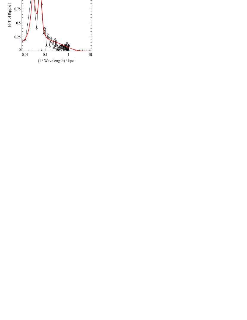
Figure 4: Positive frequency half of the Fourier transform of the fractional ripples in the Perseus cluster (points) and in our model (thick red line).

For our subsequent analysis, we often wish to compare results from model clusters to those obtained for the Perseus cluster data. Therefore we construct a fiducial model for the ripple power spectrum which is based on the spectrum observed in the Perseus cluster. We use the surface-brightness data shown in Fig. 3 of Sanders & Fabian (2007). This profile was generated in a sector with an opening angle of approximately $0.13\times 2\pi$, which we assume throughout this paper is a typical angle over which ripples will be coherent enough to allow a profile to be constructed from circular annuli. The model spectrum along with the actual Perseus spectrum is shown in Fig. 4. The model is of the form:

$$|\mathscr{F}(R(r))|=(1-e^{-ak})*(L_{0}(k)+L_{1}(k)+B*e^{-ck})$$ (12)

where $k$ is defined as $1/\lambda$ and $L_{0}$ and $L_{1}$ are Lorentzian functions representing the main peaks in the surface brightness profile:

$$L(k)=\frac{A\Gamma}{2\pi\left((x-x_{0})^{2}+\Gamma^{2}/4\right)}$$ (13)

Owing to the large number of free parameters in the model, the fit to the Perseus model was performed by eye, aiming to recreate the main features of the profile rather than provide an exact representation.

3.4 Results

3.4.1 Observation Time to Detect Ripples in Perseus

As a test of our method, we calculate the time required to detect ripples in the Perseus cluster. The projected beta models were fitted over the radius range $10-80{\rm\thinspace kpc}$, and only ripples in this range were counted.

Fig. 5 shows the expected number of ripples detected against observing time for the Perseus cluster data. Each line represents a different choice for the number of significant excesses/decrements in emission needed to count a feature as a ripple. To account for the random nature of the Poisson noise added to our degraded surface brightness profiles, we have averaged the results over several realisations of the counts profile. For the case where 2-3 adjacent features are needed to constitute a ripple, we start to see several ripple-like features detected to $3\sigma$ significance in about $40-100{\rm\thinspace ks}$, broadly compatible with the bounds $20{\rm\thinspace ks}<t<200{\rm\thinspace ks}$ imposed by the observed (non)detection times for ripples in Perseus.

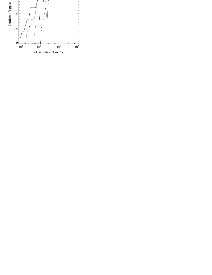
Figure 5: Number of ripples against observation time for the Perseus cluster with a detection requiring one (solid line), two (dashed line), three (dotted line) and four (dash-dotted) line features significant at the $3\sigma$ level.

Fig. 6 shows the average number of ripples detected against time for a set of model clusters with the same ripple power-spectrum as Perseus. Again the different lines represent a different number of adjacent features needed to constitute a ripple. The number of ripples detected as a function of time is comparable between the Perseus data and the model. In the case where a single feature counts as a several ripples are detected in just over $20{\rm\thinspace ks}$, but in the more realistic case where $2-3$ adjacent features are needed to identify a ripple detections take $40-100{\rm\thinspace ks}$.

Figure 6: Number of ripples detected against observation time for an average over model clusters with ripples having the same power spectrum as the Perseus cluster, with a detection requiring one (solid line), two (dashed line), three(dotted line) and four (dash-dotted) line features significant at the $3\sigma$ level.

3.4.2 Variation of Detection Time with Total Flux

In order to determine how the time to detect a ripple varies with various parameters of the underlying surface brightness and the ripple structure, we use a binary search over the observation time. At each observation time, several realisations of the model cluster are constructed and we use the algorithm discussed above to search for ripples in the region $r>10{\rm\thinspace kpc}$. At each time, we determine whether the median number of ripples detected is higher or lower than some threshold. The time for the next step is chosen as half time between the shortest time in which a detection has been made and the longest time in which no detection has been made. Initially we assume that ripples will always be detected in $10^{7}{\rm\thinspace s}$ and will never be detected in $10^{4}{\rm\thinspace s}$ (violation of these assumptions will lead to points lying just above the minimum or just below the maximum time, which will be obvious in the results). We typically consider an average of three ripple to be a detection and require at least two adjacent significant features to define a ripple.

We use the same Perseus-like model cluster as before, with the same radial bins. This is necessarily an approximation; in reality one might choose larger bins for a fainter cluster. At each observation time, 10 model clusters are generated to calculate the average number of ripples.

Fig. 7 shows two independent determinations of this variation in the required detection time with the total flux of the cluster. The error bars represent the accuracy at which the binary search is terminated, that is, the difference between the maximum observation time for a non-detection and the minimum for a detection. To gauge the uncertainty in the detection time predicted by this method, we may simply compare points from the independent runs; these seem to agree well, with the discrepancies being similar in magnitude to the plotted error bars, indicating that we are terminating the binary search at a sensible accuracy.

The detection time calculated for a Perseus-like cluster, with a flux of $6.75$ counts per second inside $100{\rm\thinspace kpc}$ is $\sim 40{\rm\thinspace ks}$.

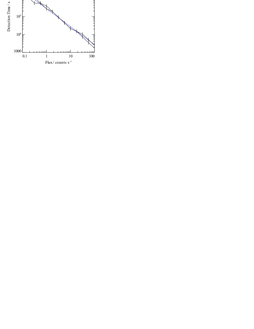
Figure 7: Two runs of the time required to detect Perseus-like ripples against the cluster flux in the detection region inside $100{\rm\thinspace kpc}$. The dashed line shows $t\sim\text{flux}^{-1}$, as expected from equation (10), and is not a fit but is normalised for a detection time of $40{\rm\thinspace ks}$ for the Perseus cluster (with a flux of $6.75{\rm\thinspace ct\ s^{-1}}$ inside $100{\rm\thinspace kpc}$ in the appropriate sector). The error bars account only for the accuracy of the binary search, not for the uncertainty in the time needed to make the detection.

3.4.3 Variation in the Detection Time With Ripple Amplitude

Fig. 8 shows to independent calculations of the detection time for various ripple amplitudes. The scaling of the detection time with ripple amplitude is roughly $t\sim\text{amplitude}^{-2}$, the same as lowest order in $f$ of equation (10).

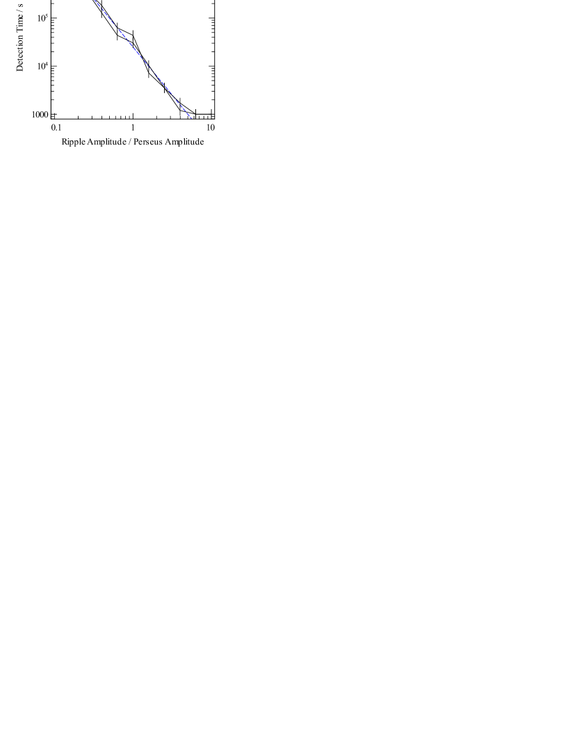
Figure 8: Two runs of the time required to detect Perseus-like ripples against the ripple amplitude. The dashed line shows $t\sim\text{amplitude}^{-2}$ scaled so the detection time at the Perseus ripple amplitude is $40{\rm\thinspace ks}$.

3.4.4 Variation in Detection Time with Ripple Wavelength

In order to determine the variation in detection time with the ripple amplitude, we took the fiducial model and altered the values of $x_{0}$ in the two Lorentzian peaks, keeping the ratio of the two wavelengths constant, whilst leaving the rest of the spectrum unaltered. This is inevitably an over-simplification; the underlying ripple wavelength is determined by the inflation process, which will also affect the other frequency components. Also, as discussed in section 2, a ripple of smaller wavelength and equal amplitude in projection corresponds to a larger amplitude ripple in 3D.

Figure 9: Two runs of the time required to detect Perseus-like ripples against the ripple wavelength. The wavelength shown corresponds to the highest frequency Lorentzian peak in the model.

Fig. 9 shows the variation in detection time with the ripple wavelength. The detection time appears to be almost independent of wavelength above wavelengths of about $8{\rm\thinspace kpc}$. This result is inconsistent with a naive prediction; the number of counts in the peak of a ripple is $N\sim SA$ where $S$ is the surface brightness at the ripple radius and $A$ is the area covered by the ripple. Typically, we have $S\sim r^{-1}$ so $N\sim r^{-1}r\lambda\sim\lambda$, and so we expect the time to detect the ripple scales like $\sim 1/\lambda$. To understand this discrepancy, we have run simulations using a simple monochromatic ripple profile, shown in Fig. 10. With monochromatic waves, the detection time more closely follows $t\sim 1/\lambda$ out to large ripple wavelengths. There is also some evidence that the beta-model underlying profile has larger detection times at radii above $r\sim r_{\text{core}}$ than the scale-free power-law model.

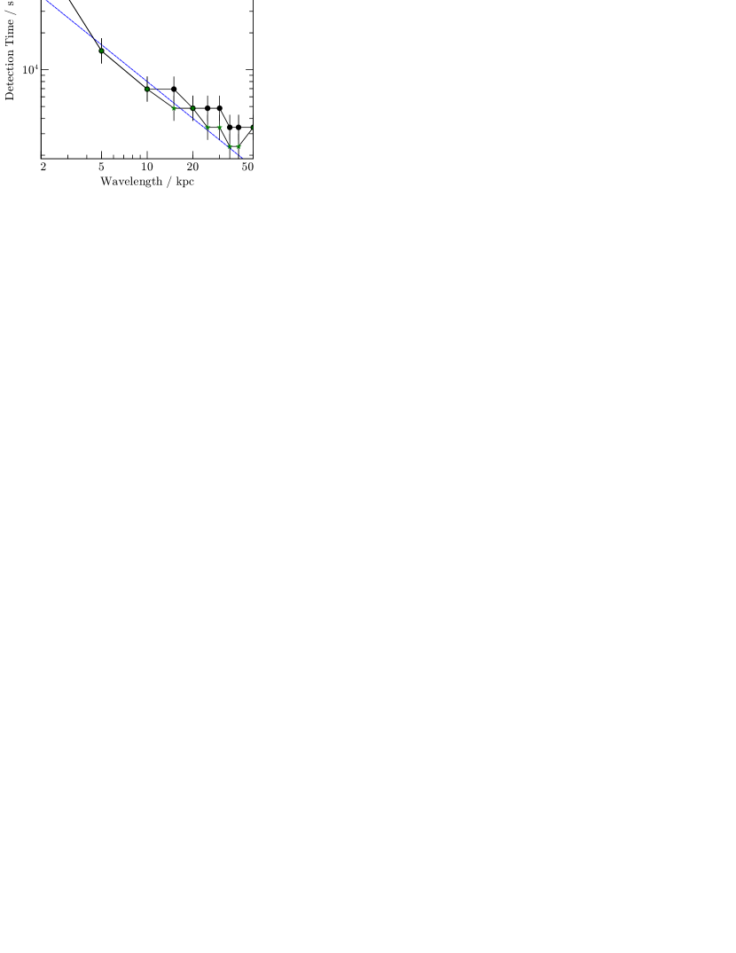
Figure 10: Time to detect monochromatic ripples against the ripple wavelength for underlying surface brightness profiles of beta model form with $r_{\text{core}}=10{\rm\thinspace kpc}$ (circles) and with a power-law profile (green stars). The profiles are scaled so that the detection times at $r=10{\rm\thinspace kpc}$ are similar. The blue dashed line indicates $t\sim\lambda^{-1}$.

3.4.5 Variation in Detection Time with Underlying Cluster Properties

Figure 11 shows the variation in detection time with the $\beta$ parameter of the underlying beta model. For reasonable values of $\beta$ there is little evidence of a substantial change in the detection time, although the time becomes large for very large $\beta$ values. Variations in the core radius of the beta model similarly make little difference to the results.

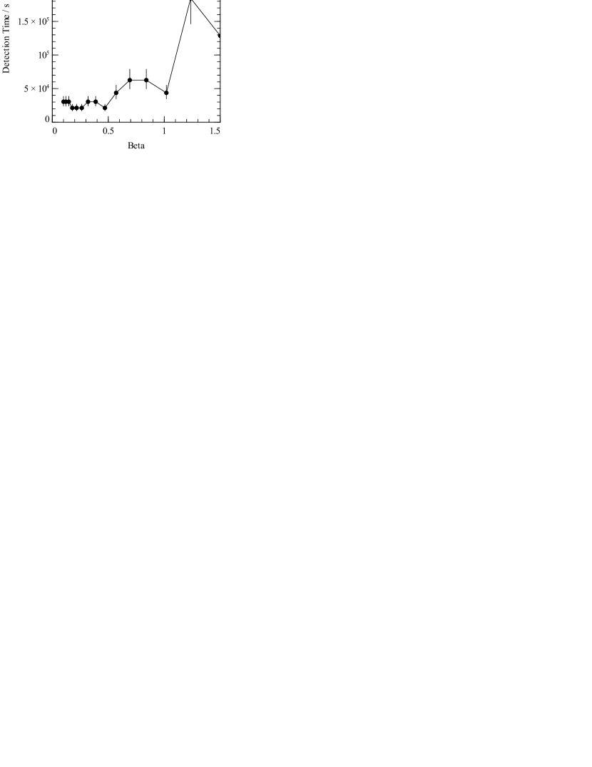
Figure 11: Mean time for detection against underlying cluster beta parameter.

3.4.6 Variation in Detection Time With Redshift

Fig. 12 shows the variation of detection time with redshift at constant flux. This means that redshift variations correspond to a rescaling of the cluster’s physical dimensions. For the cluster parameters and range of redshifts shown, the detection time does not vary significantly, however there will be a point where the wavelength of the ripple is comparable to the size of the angular bins at the cluster redshift. After this point, which will occur at smaller redshift for smaller wavelength, the ripples will become significantly more difficult to detect.

Figure 12: Mean time for detection against cluster redshift, assuming the cluster flux is constant, independent of redshift.

4 Discussion

4.1 Time Needed to Detect Ripples

Assuming that the different parameters in section 3.4 may be treated independently, we may derive a simple analytical approximation for the time to detect ripples in a given cluster. If we assume that the ripples are long enough wavelength that the scaling of detection time with ripple wavelength may be ignored, the only strong dependencies seen are with flux and amplitude, which scale in a manner consistent with the simple analytical model; $t\sim\text{flux}^{-1}$ and $t\sim\text{amplitude}^{-2}$. Taking the normalisation from the Perseus model:

$$t=40\left(\frac{f}{f_{\text{Perseus}}}\right)^{-1}\left(\frac{a}{a_{\text{Perseus}}}\right)^{-2}{\rm\thinspace ks}$$ (14)

for a cluster of flux $f$ and ripple amplitude $a$. Except for the wavelength scaling, this result is very close to the analytic prediction of (10), with the normalization increased by a factor $\sim 3.5$.

4.2 Detectability of sound waves in nearby clusters

To investigate the feasibility of detecting ripples in clusters other than Perseus using the current generation of X-ray satellites, we have used equation (14) to determine the regions of $a/a_{\text{Perseus}}$, $f/f_{\text{Perseus}}$ parameter space accessible to Chandra observations of different lengths. We have then estimated appropriate values for $a/a_{\text{Perseus}}$ and $f/f_{\text{Perseus}}$ for several nearby clusters.

To estimate $f/f_{\text{Perseus}}$, we need the flux in ${\rm\thinspace ct\ s^{-1}}$ over the region where ripples could be detected in the cluster. We assume this corresponds to the region $2r_{\text{bubble centre}}-5_{\text{bubble centre}}$ , where $r_{\text{bubble centre}}$ is the average radius of the bubble from the centre of the cluster taken from Dunn & Fabian (2004) and Dunn et al. (2005). Making different assumptions about where the flux should be measured does not change our results substantially. To measure the flux, we use raw Chandra events files taken from observations in the Chandra archive. In all cases except Virgo, the observations are taken with the ACIS-S instrument; for Virgo we scale from ACIS-I to ASIS-S by increasing the count rate by a factor 1.5 appropriate for a $3{\rm\thinspace keV}$ plasma. The energy range is limited to $0.5-7{\rm\thinspace keV}$. In each case, obvious point sources in the region of interest were removed by eye and a blank-sky background scaled to the correct exposure time and area was subtracted.

To estimate the amplitude of the ripples, we use the relationship between the power in a sound wave and its pressure amplitude Landau & Lifshitz (1959):

$$P_{\text{wave}}=4\pi r^{2}\frac{(\delta p)^{2}}{\rho c}$$ (15)

Assuming that the effect of projection is to reduce the projection reduces the surface brightness perturbation so $\delta S/S=\kappa\delta n/n$ – as discussed in Section 2 – the amplitude of surface brightness fluctuations is related to the power in the wave as:

$$\frac{\delta S}{S}=\frac{\kappa P_{\text{wave}}^{\frac{1}{2}}}{\sqrt{4\pi\gamma^{3/2}}r}\left(\frac{\rho}{p^{3}}\right)^{\frac{1}{4}}$$ (16)

To estimate the wave power in this expression, we make use of two approaches; an estimate that $P_{\text{wave}}=P_{\text{cavity}}$ based on the cavity power using the buoyancy timescale Bîrzan et al. (2004); Dunn & Fabian (2004); Rafferty et al. (2006) and an estimate $P_{\text{wave}}=L_{\text{cool}}(1-2r_{\text{bubble}}/r_{\text{cool}})$. The factor $(1-2r_{\text{cool}}/r_{\text{bubble}})$ is to account for the fact that the very central region of the cluster is not likely to be heated by sound waves but instead by weak shocks and cavity heating (McNamara & Nulsen, 2007). To estimate the projection factor $\kappa$, we assume that the dominant ripple wavelength is $\sim 2r_{\text{b}}$ i.e. twice the average bubble dimension; this is a good approximation for the Perseus cluster. $\kappa$ is then calculated using the procedure in section 2. We take $r$ to be $5r_{\text{bubble centre}}$.

Using this model, with the cluster and bubble properties presented in Dunn & Fabian (2004, 2006) assuming that the cavity power is $4pV$ appropriate if the bubbles are filled with a fully-relativistic plasma, we predict the value of $\delta S/S$ for several local clusters, which we compare to $\delta S/S=0.05$ for the Perseus cluster. Fig. 13 shows the position of these clusters on a flux-amplitude plane, including values for the Perseus cluster both calculated from this model and from the actual observations. The corresponding detection times with Chandra are indicated by the shaded regions.

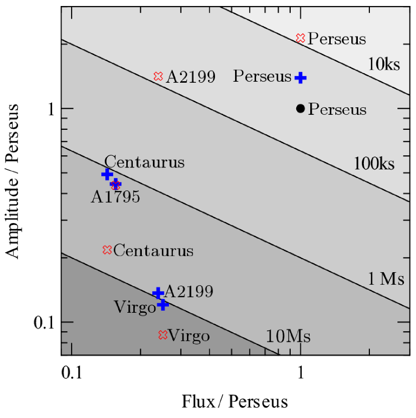
Figure 13: Flux and predicted ripple amplitude of some local clusters compared to Perseus. Blue plusses are based on the X-ray luminosity within the cluster cooling radius, red crosses are an estimate based on the cavity power. The black circle indicates the observed position of the Perseus cluster. Shaded regions indicate the predicted detection times for sound waves in the clusters using Chandra.

The above analysis suggests that detecting ripples in several local clusters may be possible with the Chandra satellite. In particular Centaurus, Abell 1795 and Abell 2199 are promising candidates for detections in around $1{\rm\thinspace Ms}$ of observation time. However it is important to note that there is considerable uncertainty in the wave amplitude determined for each cluster, with the two calculated estimates giving up to an order of magnitude difference in the estimated amplitude. In Perseus it is apparent that the cooling luminosity is a better estimator of the wave amplitude than the cavity power, which is likely true for other clusters if the power in sound wave is closer to the time-average heating power than the instantaneous cavity power.

In addition to the power estimates, there are also uncertainties associated with the ripple wavelength and the radius at which it is assumed that the detection will be made. For a cluster like Centaurus which is currently under-heated by the cavities, the final size of the bubbles is likely greater than the current size; Dunn & Fabian (2006) estimate $r_{\text{b}}/r_{\text{b, max}}=0.75$ for Centaurus, although it is notable that many clusters in their sample have $r_{\text{b}}/r_{\text{b, max}}>1$, indicating the cavities grow larger than needed to offset the cooling. Increasing the bubble radius will increase the wavelength of the ripples generated by the cavity inflation, reducing the projection factor for the ripples. For Centaurus, increasing the wavelength by a factor 1.5 would reduce the time needed to detect the waves by a factor of $\sim 2.25$ to a few hundred kilo-seconds. Conversely, the most prominent bubbles in Abell 2199 are likely detached from the central source and buoyantly rising in the ICM. Therefore their dimensions likely overestimate the ripple wavelength and excluding the region inside $2r_{\text{bubble centre}}$ probably underestimates the cooling luminosity. This may explain the large discrepancy between the cooling luminosity and cavity luminosity based estimates of the amplitude in this system.

Detection times may also increase if the cluster is in a regime where the wavelength of the ripples is important; for example if it has astrongly monochromatic ripples so the detection time scales as $\sim 1/\lambda$.

Given the large uncertainty on the amplitude of the waves, and the strong dependence of the detection time on the amplitude, it may be possible to see ripples in some local clusters with currently available data. In Abell 2199, an isothermal shock has been seen in a $33{\rm\thinspace ks}$ exposure, but an unsharp-mask analysis revealed no further ripple-like features. For Centaurus, $200{\rm\thinspace ks}$ of Chandra data are available, and have been analysed for ripples by Sanders et al. (in prep.).

It is also important to recognise the limitations of our predictions compared to the procedure that has been used to find ripples in practice. The starting place to locate ripples in practice will be an image of the cluster such as Fig. 1 in which the small-scale features have been brought out using a technique such as unsharp-masking or a Fourier-filter. Assuming ripples exist in the cluster, whether they are seen in the resulting image will depend substantially on the degree of coherence of the ripples and the complexity of the radial power spectrum of the ripples. Ripples with a high degree of coherence might be discovered in much less time than suggested by our analysis whilst those with a limited degree of coherence might not be noticed even in very long exposures. Since coherent features are likely easier to identify with better spatial resolution this suggests ripples will be easier to detect in low-redshift clusters than in higher redshift clusters even where their observed flux is similar.

Related to this issue is that of the threshold number of standard deviations from the background count rate needed to class a feature as a ripple. In our analysis, we have assumed each feature needs to be detected to $3\sigma$. In practice, detecting a large number of clearly ripple-like features to less than $3\sigma$ may be a more convincing detection than a detection in which a few blobs are detected to higher significant, but the intermediate structure is not clearly ripple-like.

Given these limitations, extreme caution must be made in predicting exact detection times for ripples and for interpreting non-detections as indicating that no ripple-like structures exist in a given cluster.

5 Conclusion

In order to understand the role played by sound waves in distributing energy in cluster cores, it is essential to study these waves in a variety of cluster systems. To understand the requirements for such a study, we have investigated the effect of projection on reducing the observed wave amplitude compared to the intrinsic amplitude in a range of cluster atmospheres, and we have calculated the detection times for waves in a number of cluster environments.

Projection of ripples in the emissivity profile substantially reduces the amplitude of the surface brightness ripples. The magnitude of this effect is a strong function of the ripple wavelength, but depends little on the underlying atmosphere properties. If the wavelength of the ripples is correlated with the dimensions of the cavity, this implies systems with larger cavities may be more promising targets for the detection of ripples.

By constructing an algorithm for detecting ripples in model data, we have shown that the detection time for Perseus-like surface brightness ripples is critically determined by two features of the cluster – the total flux and the ripple amplitude. Other factors such as the underlying cluster properties have a much more limited effect. Applying our results to nearby clusters, and assuming that the ripple amplitude is sufficient to heat the cluster, we estimated detection times for ripples using the Chandra satellite.

These detection times suggest that a selection of nearby, bright clusters may contain ripples detectable in around $\sim 1{\rm\thinspace Ms}$ of Chandra observation time, although there is considerable uncertainty brought about by uncertainties in the expected amplitude of the ripples. In cooler clusters such as Virgo that require less heating, and so are expected to have smaller ripples, the detection times are likely prohibitively long with Chandra but should be well within reach of XEUS which promises one to two orders of magnitude greater effective area.

6 Acknowledgements

ACF thanks the Royal Society for support.

References

- Bîrzan et al. (2004) Bîrzan L., Rafferty D. A., McNamara B. R., Wise M. W., Nulsen P. E. J., 2004, ApJ, 607, 800
- Böhringer et al. (1993) Böhringer H., Voges W., Fabian A. C., Edge A. C., Neumann D. M., 1993, MNRAS, 264, L25
- Cavaliere & Fusco-Femiano (1976) Cavaliere A., Fusco-Femiano R., 1976, A&A, 49, 137
- Dunn & Fabian (2004) Dunn R. J. H., Fabian A. C., 2004, MNRAS, 355, 862
- Dunn & Fabian (2006) Dunn R. J. H., Fabian A. C., 2006, MNRAS, 373, 959
- Dunn et al. (2005) Dunn R. J. H., Fabian A. C., Taylor G. B., 2005, MNRAS, 364, 1343
- Ettori (2000) Ettori S., 2000, MNRAS, 318, 1041
- Fabian et al. (2003) Fabian A. C., Sanders J. S., Allen S. W., Crawford C. S., Iwasawa K., Johnstone R. M., Schmidt R. W., Taylor G. B., 2003, MNRAS, 344, L43
- Fabian et al. (2006) Fabian A. C., Sanders J. S., Taylor G. B., Allen S. W., Crawford C. S., Johnstone R. M., Iwasawa K., 2006, MNRAS, 366, 417
- Landau & Lifshitz (1959) Landau L. D., Lifshitz E. M., 1959, Fluid mechanics. Course of theoretical physics, Oxford: Pergamon Press, 1959
- McNamara & Nulsen (2007) McNamara B. R., Nulsen P. E. J., 2007, ARA&A, 45, 117
- Peterson & Fabian (2006) Peterson J. R., Fabian A. C., 2006, Physics Reports, 427, 1
- Peterson et al. (2003) Peterson J. R., Kahn S. M., Paerels F. B. S., Kaastra J. S., Tamura T., Bleeker J. A. M., Ferrigno C., Jernigan J. G., 2003, ApJ, 590, 207
- Rafferty et al. (2006) Rafferty D. A., McNamara B. R., Nulsen P. E. J., Wise M. W., 2006, ApJ, 652, 216
- Sanders & Fabian (2007) Sanders J. S., Fabian A. C., 2007, MNRAS, 381, 1381