QCD AT COMPLEX COUPLING, LARGE ORDER IN PERTURBATION THEORY AND THE GLUON CONDENSATE

Abstract

We discuss the relationship between the large order behavior of the perturbative series for the average plaquette in pure gauge theory and singularities in the complex coupling plane. We discuss simple extrapolations of the large order for this series. We point out that when these extrapolated series are subtracted from the Monte Carlo data, one obtains (naive) estimates of the gluon condensate that are significantly larger than values commonly used in the continuum for phenomelogical purpose. We present numerical results concerning the zeros of the partition function in the complex coupling plane (Fisher’s zeros). We report recent attempts to solve this problem using the density of states. We show that weak and strong coupling expansions for the density of states agree surprisingly well for values of the action relevant for the crossover regime.

1 Motivations

Perturbation theory has played a major role in the establishment of the standard model of electro-weak and strong interactions. However, it is well known [1] that perturbative series have a zero radius of convergence and that at some critical order, adding more terms does not improve the accuracy of the result.

There exists a connection between large field configurations and the large order of perturbative series [2] that can be illustrated with the simple integral

$$\int_{-\infty}^{+\infty}d\phi e^{-\frac{1}{2}\phi^{2}-\lambda\phi^{4}}\neq\sum_{0}^{\infty}\frac{(-\lambda)^{l}}{l!}\int_{-\infty}^{+\infty}d\phi e^{-\frac{1}{2}\phi^{2}}\phi^{4l}$$ (1)

The truncation of the exponential at order $l$ is justified if the argument is much smaller than $l$. However, the peak of the integrand is located at $\phi=\sqrt{4l}$. For this value of $\phi$, the argument of the exponential is $\lambda 16l^{2}$, which for $l$ large enough will be larger than $l$. In other words, the peak of the integrand of the r.h.s. moves too fast when the order increases. On the other hand, if we introduce a field cutoff, the peak moves outside of the integration range and

$$\int_{-\phi_{max}}^{+\phi_{max}}d\phi e^{-\frac{1}{2}\phi^{2}-\lambda\phi^{4}}=\sum_{0}^{\infty}\frac{(-\lambda)^{l}}{l!}\int_{-\phi_{max}}^{+\phi_{max}}d\phi e^{-\frac{1}{2}\phi^{2}}\phi^{4l}$$ (2)

This example suggests that one should use perturbation theory to treat small quantum fluctuations and semi-classical methods to treat the large field configurations.

For QCD, an important challenge is to describe the large distance behavior of the theory in terms of degrees of freedom which are weakly coupled at short distance. This question can be addressed in the framework of the lattice formulation. We consider the simplest case of Wilson’s action which is the sum over the plaquettes in the fundamental $SU(N)$ representation:

$$S=\sum_{p}(1-(1/N)ReTr(U_{p}))\ .$$ (3)

With the usual notation $\beta=2N/g^{2}$, the partition function reads

$$Z=\prod_{l}\int dU_{l}{\rm e}^{-\beta S}\ .$$ (4)

For $N=3$, this theory has no phase transition when one goes from small coupling (large $\beta$) to large coupling (small $\beta$). Recently, convincing argument have been given [3, 4] in favor of the smoothness of the RG flows between the two corresponding fixed points. Consequently, there does not seem to exist any fundamental obstruction to match the two regimes. One general question that we would like to address is if it is possible to construct a modified weak coupling expansion that could bridge the gap to the strong coupling regime.

Lattice gauge theories with a compact group have a build-in large field cutoff: the group elements associated with the links are integrated with $dU_{l}$, the compact Haar measure. For $SU(2)$ and $SU(3)$, the action density has an upper bound which is saturated when the group element is a nontrivial element of the center. It is remarkable that this formulation has a UV regularization and a large field regularization that preserves gauge invariance. Does the presence of large field cutoff means that perturbative series are convergent? Not necessarilly, because in constructing perturbative series, one decompactifies [5] the gauge field integration which at low order amounts to neglect exponentially small tails of integration, but modifies the large order drastically.

In continuous field theories, it is expected [6, 7, 8, 9] that the large order of perturbative series can be calculated from classical solutions at small negative $\lambda$ for scalar theories or small negative $g^{2}$ for gauge theories. For lattice gauge theory with compact groups, the theory is mathematically well defined at negative $g^{2}$ ,i. e., negative $\beta$, but some Wilson loops oscillate when their size change and the average plaquette has a discontinuity when $g^{2}$ changes sign[10]. For small negative $g^{2}$, i. e., large negative $\beta$, the behavior of expectation values is dominated by the large field configurations. This statement can be made more precise by introducing the spectral decomposition

$$Z=\int_{0}^{S_{max}}dS\ n(S){\rm e}^{-\beta S}\ ,$$ (5)

with $n(S)$ the so-called density of states. It is clear that for large negative $\beta$, what matters is the behavior of $n(S)$ near $S_{max}$.

We can make the discussion more concrete by considering the case of the single plaquette model [11] with $SU(2)$ gauge group. In this case, $S_{max}=2$ and we have

$$n_{1pl.}(S)=\frac{2}{\pi}\sqrt{S(2-S)}\ .$$ (6)

The weak coupling expansion of $Z$ is determined by the behavior of near $S=2$. When we expand $\sqrt{2-S}$ about $S=0$, the large order of this series is determined by the cut at $S=2$. After integration (from 0 to $+\infty$) over $S$, the series with a finite radius of convergence becomes asymptotic (inverse Borel transform). Alternatively, we can maintain the finite range of integration and construct a converging weak coupling expansion but with coupling dependent coefficients as done by Hadamard a century ago in his study of Bessel functions. It would be interesting to know if the features of the one plaquette model persist in the infinite volume limit of lattice gauge theory.

In these proceedings, we discuss the large order behavior of the weak coupling expansion of the plaquette (Sec. 2) and the possibility of defining its non-perturbative part (the gluon condensate? Sec. 3) . More details can be found in Ref. [12]. In Sec. 4, we present numerical results concerning the zeros of the partition function in the complex coupling plane [13, 14] (Fisher’s zeros). This problem could be solved using the density of states. Preliminary numerical results concerning the density of states are provided in Sec. 5 where we also show that weak and strong coupling expansions for the density of states agree surprisingly well for values of the actions relevant for the crossover regime. After the conference, we wrote a more detailed preprint [15] concerning this question.

2 Perturbative series in lattice gauge theory

In this section, we denote $\mathcal{N}_{p}\equiv\ L^{D}D(D-1)/2\$ the number of plaquettes and the average plaquette:

$$P(\beta)=(1/\mathcal{N}_{p})\left\langle\sum_{p}(1-(1/N)ReTr(U_{p}))\right\rangle\ .$$ (7)

The weak coupling expansion of this quantity

$$P(\beta)\simeq\sum_{m=1}b_{m}\beta^{-m}+\dots.$$ (8)

has been calculated up to order ten [16] and 16 [17]. Series analysis [18, 19] suggest a singularity $P\propto(1/5.74-1/\beta)^{1.08}$ and consequently a finite radius of convergence. This is not expected since the plaquette changes discontinuously [10] at $\beta\rightarrow\pm\infty$. This behavior is also not seen in the 2d derivative of $P$ and would require massless glueballs.

A simple alternative is that the critical point in the fundamental-adjoint plane [20] has mean field exponents and in particular $\alpha=0$. On the $\beta_{adj.}=0$ line, we assume an approximate logarithmic behavior (mean field)

$$-\partial P/\partial\beta\propto{\rm ln}((1/\beta_{m}-1/\beta)^{2}+\Gamma^{2})\ .$$ (9)

$\Gamma$ cannot be too small (absence of singularities) or too large (this would create visible oscllations in the perturbative coefficients). From these constraints, we get the approximate bounds [12] $0.001<\Gamma<0.01$.

Integrating, we get the approximate form

$$\sum_{k=0}b_{k}\beta^{-k}\simeq C({\rm Li}_{2}(\beta^{-1}/(\beta_{m}^{-1}+i\Gamma))+{\rm h.c}\ ,$$ (10)

with

$${\rm Li}_{2}(x)=\sum_{k=0}x^{k}/k^{2}\ .$$ (11)

We fixed $\Gamma=0.003$ and obtained $C=0.0654$ and $\beta_{m}$=5.787 using of $b_{9}$ and $b_{10}$. The low order coefficients depend very little on $\Gamma$ (when $\Gamma<0.01$), larger series are needed to get a better estimate of $\Gamma$ for $SU(3)$. It interesting to notice that we get very good predictions of the values of $b_{8},b_{7},\dots$!

Predicted values of $b_{m}$ with the dilog model. order predicted numerical [16] rel. error 1 0.7567 2 -0.62 2 1.094 1.2208 -0.10 3 2.811 2.961 -0.05 4 9.138 9.417 -0.03 5 33.79 34.39 -0.017 6 135.5 136.8 -0.009 7 575.1 577.4 -0.004 8 2541 2545 -0.0016 9 exact 11590 10 exact 54160

We believe that these regularities should have a Feynman diagram interpretation.

Another possible model [21, 22] is based on IR renormalons

$$\sum_{k=0}b_{k}\bar{\beta}^{-k}\simeq K\int_{t_{1}}^{t_{2}}dt{\rm e}^{-\bar{\beta}t}\ (1-t\ 33/16\pi^{2})^{-1-204/121}$$ (12)

$$\bar{\beta}=\beta(1+d_{1}/\beta+\dots)$$ (13)

$t_{1}=0$ corresponds to the UV cutoff while $t_{2}=16\pi^{2}/33$ corresponds to the Landau pole. For $t_{2}=\infty$ we get a perturbative series with a factorial growth, in contrast with the previous model which had a power growth. Unfortunately a clear distinction between the two types of large order behavior requires numerical calculations at order larger than 20.

3 The Gluon Condensate

Using the two large order extrapolations described in the previous section, one can see good evidence [12] for

$$P(\beta)-P_{pert.}(\beta)\simeq B(a/r_{0})^{4}\ ,$$ (14)

with $a(\beta)$ defined with the so-called force scale, [23, 24] and $P_{pert}$ appropriately truncated for the second model. $B$ is sensitive to resummation. $B\simeq 0.7$ with the bare series [12] and 0.4 with the tadpole improved series [17].

It is tempting but potentially dangerous to try to relate $B$ to the numerical value of the gluon condensate[25]. If we identify [26] for $N=3$

$$P(\beta)-P_{pert.}(\beta)\simeq a^{4}\frac{\pi^{2}}{36}<\frac{\alpha}{\pi}GG>,$$ (15)

we obtain for $r_{0}=0.5\ fm$ and $B=0.4$ that $<\frac{\alpha}{\pi}GG>\simeq 0.035\ GeV^{4}$ which is about 3 times the original estimate[25]. It is not clear to us that there is a precise correspondence between the continuum and the lattice definitions. Also, different values for the continuum value have been proposed. A negative value [27], subsequently criticized [28] can even be found. For these reasons, some authors [29] prefer to use a value 0 with error bars when estimating $\alpha_{s}$ at some large scale. If we use the correspondence between the lattice and the continuum discussed above at face value with $B=0.4-0.7$, these error bars should be multiplied by a factor 3 to 6.

4 Zeros of the Partition Function

The existence of complex singularities near the real axis can be tested by studying the complex zeros of the partition function [30]. The basic technique is the reweighting [31, 32] of action distributions at given $\beta_{0}$

$$Z(\beta_{0}+\Delta\beta)=Z(\beta_{0})<\exp(-\Delta\beta S)>_{\beta_{0}}\ .$$ (16)

As mentioned in the introduction, $Z(\beta)$ is the Laplace transform of the density of states $n(S)$. For $SU(2)$ with even numbers of sites in each direction [10] $Z(-\beta)={\rm e}^{2\beta\mathcal{N}_{p}}Z(\beta)$ and $n(S)=n(2\mathcal{N}_{p}-S)$. In the crossover, we have attempted local parametrizations [13, 14]:

$$n(S)\propto{\rm e}^{-(a_{1}S+a_{2}S^{2}+a_{3}S^{4}+a_{4}S^{4})}$$ (17)

For $SU(3)$ on a $4^{4}$ lattice, stronger deviations from the Gaussian behavior are observed than for $SU(2)$. This is illustrated in Fig. 1 that has a larger scale than its $SU(2)$ counterpart. The histogram were made with 50,000 configurations prepared for a study of the third and fourth moments [19]. As the volume increases, these features tend to disappear in the statistical noise.

Figure 1: The relative difference with a Gaussian distribution for 50,000 values of $S$ in an histogram with 100 bins for a $SU(3)$ pure gauge theory on $4^{4}$ and $6^{4}$ lattices at $\beta=5.58$ .

These local model give results that can be compared to MC reweighting in the region where the errors on the zero level curves for the real and imaginary parts are not too large [13]. An important consistency test is to show that approximately the same zeros are obtained for different $\beta_{0}$. This is illustrated in Fig. 2. We plan to pursue this study using the more global information provided by the density of states.

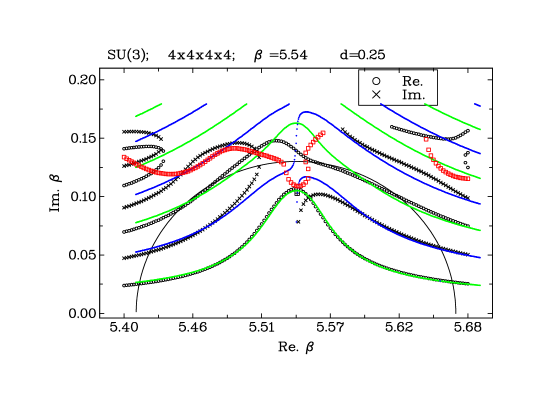
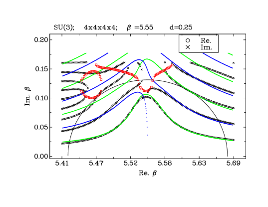
Figure 2: Zeros of the real (circles) and imaginary (crosses) for $SU(3)$ on a $4^{4}$ lattice using reweighting of MC data at $\beta_{0}$ = 5.54 and 5.55. The small dots are the values for the real (green) and imaginary (blue) parts obtained from the 4 parameter model. The crossed box at ((5.541,0.103) above and (5.542,0.102) below) have been obtained with a perturbative method. Red boxes: boundary of the MC confidence region. The solid line is the circle of confidence of the Gaussian approximation. The locations of the complex zeros are consistent.

5 Approximate form of the density of state $n(S)$ for $SU(2)$

We assume the following form:

$$n(S)={\rm e}^{\mathcal{N}_{p}f(S/\mathcal{N}_{p})}\ .$$ (18)

In the infinite volume limit, $f(x)$ becomes volume independent and can be interpreted as a (color) entropy density. In the same limit, we have the saddle point equation

$$f^{\prime}(x)=\beta\ .$$ (19)

This is the analog of the familiar thermodynamical relation $dS/dE=1/T$. Knowing $f(x)$ amounts to solve the theory (in a thermodynamical sense). For $SU(2)$, $f(x)=f(2-x)$ (symmetric about 1) and we don’t need to calculate $f$ for $x>1$. We have constructed weak coupling and strong coupling expansions for $SU(2)$ and compared with numerical data on a $4^{4}$ lattice.

For the weak coupling, we use the large beta expansion near $x=0$, $x=<S/\mathcal{N}_{p}>=\frac{3}{4}\frac{1}{\beta}+0.156\frac{1}{\beta^{2}}+\dots$. We assume $f(x)\simeq A\ ln(x)+B+Cx+\dots$, plug the expansion in the saddle point equation and solve for $A$ and other unknowns. We obtained $f(x)=\frac{3}{4}ln(x)+0.208x+0.0804x^{2}+\dots$. For the strong coupling, we use the low beta expansion [33] to solve near $x=1$ for $SU(2)$, and obtained $x-1=<S/\mathcal{N}_{p}-1>=-\frac{\beta}{4}+\frac{\beta^{3}}{96}-\frac{7\beta^{5}}{1536}+\frac{31\beta^{7}}{23040}+\dots+\frac{1826017873\beta^{15}}{68491306598400}$. With periodic boundary conditions, the coefficients have no volume dependence for graphs with trivial topology (volume dependence should appear at order $\beta^{2L}$). Solving the saddle point equation for an expansion about 1, we get $f(x)=-2(x-1)^{2}-\frac{2}{3}(x-1)^{4}+\dots+\frac{163150033(x-1)^{16}}{255150}+\dots$.

The numerical construction of $n(S)$ by patching was done by A. Denbleyker and is illustrated in Fig. 3. Series expansions of $f(x)$ are compared with the numerical data in Fig. 4. Note the good agreement in the intermediate region. After the conference, we wrote a more detailed preprint [15] where details can be found.

figure=nsp.ps,width=3.in,angle=270

figure=nspatched.ps,width=3.in,angle=270

Figure 3: $n(S)\propto P_{\beta_{0}}(S){\rm e}^{\beta_{0}S}$ for different $\beta_{0}$ (patching). Collection of overlapping data (A. Denbleyker).

figure=ns.eps,width=3.in,angle=0

Figure 4: $ln(n(S))$ numerical (black), strong coupling at order 16 (blue) and weak coupling with dilog model at order 10 (green) for $SU(2)$ on a $4^{4}$ lattice.

6 Conclusions

The density of state show a nice overlapping of the strong and weak coupling expansions. We plan to use the density of states to study the Fisher’s zeros. We need numerical confirmation of guesses made for the weak coupling expansion for $SU(2)$ where $Im\beta_{F}/Re\beta_{F}$ is 5 times larger than for $SU(3)$ . We need better understanding of the lattice and the continuum definitions of the gluon condensate. We need a better understanding of the large order behavior of QCD series in terms of the behavior at small complex coupling (a picture analog to metastability at $\lambda<0$ for the anharmonic oscillator [6, 7, 8, 9]).

This research was supported in part by the Department of Energy under Contract No. FG02-91ER40664.

References

- [1] F. Dyson, Phys. Rev. 85, p. 631 (1952).
- [2] Y. Meurice, Phys. Rev. Lett. 88, p. 141601 (2002).
- [3] E. T. Tomboulis, arXiv 0707.2179 (2007).
- [4] E. T. Tomboulis, PoS LATTICE2007, p. 336 (2007).
- [5] U. M. Heller and F. Karsch, Nucl. Phys. B251, p. 254 (1985).
- [6] C. Bender and T. T. Wu, Phys. Rev. 184, p. 1231 (1969).
- [7] G. Parisi, Phys. Lett. 68B, p. 361 (1977).
- [8] E. Brezin, J. L. Guillou and J. Zinn-Justin, Phys. Rev. D 15, p. 1544 (1977).
- [9] J. C. LeGuillou and J. Zinn-Justin, Large-Order Behavior of Perturbation Theory (North Holland, Amsterdam, 1990).
- [10] L. Li and Y. Meurice, Phys. Rev. D 71, p. 016008 (2005).
- [11] L. Li and Y. Meurice, Phys. Rev. D71, p. 054509 (2005).
- [12] Y. Meurice, Phys. Rev. D74, p. 096005 (2006).
- [13] A. Denbleyker, D. Du, Y. Meurice and A. Velytsky, Phys. Rev. D76, p. 116002 (2007).
- [14] A. Denbleyker, D. Du, Y. Meurice and A. Velytsky, PoS LAT2007, p. 269 (2007).
- [15] A. Denbleyker, D. Du, Y. Liu, Y. Meurice and A. Velytsky, arXiv 0807.0185 (2008) (Phys. Rev. D (submitted)).
- [16] F. Di Renzo and L. Scorzato, JHEP 10, p. 038 (2001).
- [17] P. E. L. Rakow, PoS LAT2005, p. 284 (2006).
- [18] R. Horsley, P. E. L. Rakow and G. Schierholz, Nucl. Phys. Proc. Suppl. 106, 870 (2002).
- [19] L. Li and Y. Meurice, Phys. Rev. D73, p. 036006 (2006).
- [20] G. Bhanot and M. Creutz, Phys. Rev. D24, p. 3212 (1981).
- [21] A. H. Mueller Talk given at Workshop on QCD: 20 Years Later, Aachen, Germany, 9-13 Jun 1992.
- [22] F. Di Renzo, E. Onofri and G. Marchesini, Nucl. Phys. B457, 202 (1995).
- [23] M. Guagnelli, R. Sommer and H. Wittig, Nucl. Phys. B535, 389 (1998).
- [24] S. Necco and R. Sommer, Nucl. Phys. B622, 328 (2002).
- [25] M. A. Shifman, A. I. Vainshtein and V. I. Zakharov, Nucl. Phys. B147, 385 (1979).
- [26] A. Di Giacomo and G. C. Rossi, Phys. Lett. B100, p. 481 (1981).
- [27] M. Davier, S. Descotes-Genon, A. Hocker, B. Malaescu and Z. Zhang, arXiv 0803.0979 (2008).
- [28] K. Maltman and T. Yavin, arXiv 0807.0650 (2008).
- [29] C. T. H. Davies et al., arXiv 0807.1687 (2008).
- [30] M. Fisher, in Lectures in Theoretical Physics Vol. VIIC (University of Colorado Press, Boulder, Colorado, 1965), Boulder, Colorado.
- [31] M. Falcioni, E. Marinari, M. L. Paciello, G. Parisi and B. Taglienti, Phys. Lett. B108, 331 (1982).
- [32] N. A. Alves, B. A. Berg and S. Sanielevici, Phys. Rev. Lett. 64, 3107 (1990).
- [33] R. Balian, J. M. Drouffe and C. Itzykson, Phys. Rev. D11, p. 2104 (1975).