Ionizing Photon Escape Fractions from High Redshift Dwarf Galaxies

Abstract

It has been argued that low-luminosity dwarf galaxies are the dominant source of ionizing radiation during cosmological reionization. The fraction of ionizing radiation that escapes into the intergalactic medium from dwarf galaxies with masses less than $\sim$$10^{9.5}$ solar masses plays a critical role during this epoch. Using an extensive suite of very high resolution (0.1 pc), adaptive mesh refinement, radiation hydrodynamical simulations of idealized and cosmological dwarf galaxies, we characterize the behavior of the escape fraction in galaxies between $3\times 10^{6}$ and $3\times 10^{9}$ solar masses with different spin parameters, amounts of turbulence, and baryon mass fractions. For a given halo mass, escape fractions can vary up to a factor of two, depending on the initial setup of the idealized halo. In a cosmological setting, we find that the time-averaged photon escape fraction always exceeds 25% and reaches up to 80% in halos with masses above $10^{8}$ solar masses with a top-heavy IMF. The instantaneous escape fraction can vary up to an order of magnitude in a few million years and tend to be positively correlated with star formation rate. We find that the mean of the star formation efficiency times ionizing photon escape fraction, averaged over all atomic cooling ($T_{\rm vir}\geq 8000~{}$K) galaxies, ranges from 0.02 for a normal IMF to 0.03 for a top-heavy IMF, whereas smaller, molecular cooling galaxies in minihalos do not make a significant contribution to reionizing the universe due to a much lower star formation efficiency. These results provide the physical basis for cosmological reionization by stellar sources, predominately atomic cooling dwarf galaxies.

1. Introduction

In most calculations of cosmological reionization, it has to be assumed that the product of star formation efficiency and hydrogen ionizing photon escape fraction is $\geq 0.01$ (e.g. Gnedin, 2000; Cen, 2003a, b; Wyithe & Loeb, 2003a, b; Venkatesan et al., 2003; Somerville et al., 2003; Chiu et al., 2003; Haiman & Holder, 2003; Ciardi et al., 2003; Sokasian et al., 2003, 2004; Wyithe & Cen, 2007; Srbinovsky & Wyithe, 2008) in order to reionize the universe early enough to be consistent with the Wilkinson Microwave Anisotropy Probe (WMAP) observations (Spergel et al., 2007; Komatsu et al., 2008), if stars produce the majority of ionizing photons. Gnedin (2000) suggested that, based on Local Group dwarf galaxies, the star formation efficiency at high redshift is $\sim 4\%$, consistent with theoretical works (e.g. Krumholz & McKee, 2005; Krumholz & Tan, 2007). Thus, unless star formation efficiency is unusually high (i.e., $\geq 10\%$) at high redshift, this requirement seems to suggest a high ionizing photon escape fraction from high redshift galaxies, $f_{\rm esc}\geq 10\%$, may be necessary in the context of stellar reionization within the standard cold dark matter model.

However, $f_{\rm esc}\geq 10\%$ is by no means the norm, at least from observations at lower redshifts. Approximately 6% of ionizing radiation escape from the Milky Way (Bland-Hawthorn & Maloney, 1999; Putman et al., 2003). For local starburst galaxies Hurwitz et al. (1997) gave $f_{\rm esc}\leq 0.032,0.052,0.11$ ($2\sigma$) for Mrk 496, Mrk 1267, and IRAS 08339+6517 ($\leq 0.57$ in the case of Mrk 66). Deharveng et al. (2001) gave an escape fraction of $f_{\rm esc}<0.062$ for Mrk 54. Heckman et al. (2001) found $f_{\rm esc}\leq 0.06$. Bergvall et al. (2006) found $f_{\rm esc}\sim 0.04-0.1$ for a local extreme starburst dwarf, the Blue Compact Galaxy Haro 11. Chen et al. (2007) placed a 95% upper limit of $f_{\rm esc}\leq 0.075$ for star forming regions hosting gamma-ray bursts at $z\geq 2$. For Lyman break galaxies at $z\sim 3$, Shapley et al. (2006) found $f_{\rm esc}\sim 0.03$. Siana et al. (2007) examined starburst galaxies at $z\sim 1.3$ and found that less than 20% have relative escape fractions near unity and a global absolute escape fraction of $\lower 3.00003pt\hbox{$\,\buildrel<\over{\sim}\,$}0.04$. However in this study, some galaxies have upper limits of $f_{\rm esc,rel}$ as low as 0.08. Inoue et al. (2006) recently compiled available observations over a wide range of redshift and come to the conclusion that there is a trend of increasing $f_{\rm esc}$ with redshift from $\leq 0.01$ at $z\leq 1$ to $\sim 0.1$ at $z\geq 4$.

Some theoretical works also seem to point to low values for $f_{\rm esc}$. Theoretical models of our own Galaxy with realistic star formation mode by Dove et al. (2000) give an estimate of $f_{\rm esc}\sim 0.06$ or lower. Ciardi et al. (2002) studied the effect of gas inhomogeneities on $f_{\rm esc}$ for Milky Way like galaxies using simulations with radiative transfer and concluded that $f_{\rm esc}$ depends on the density structure as well as star formation rate (SFR). In addition, porosity in the interstellar medium (ISM) that is caused by SN mechanical feedback may provide additional channels in which radiation could escape, thus increasing the UV escape fraction (Clarke & Oey, 2002). Wood & Loeb (2000) argued that $f_{\rm esc}\leq 0.01$ for galaxies at $z\sim 10$. Ricotti & Shull (2000) found that $f_{\rm esc}\geq 0.1$ only for halos of total mass less than $\sim 10^{7}{\rm\,M_{\odot}}$ at $z\geq 6$ with $f_{\rm esc}$ dropping precipitously for larger halos. Fujita et al. (2003), using ZEUS-3D simulations, found that $f_{\rm esc}\leq 0.1$ from disks of dwarf starburst galaxies of total mass $M\geq 10^{8-10}{\rm\,M_{\odot}}$. Razoumov & Sommer-Larsen (2006, 2007, hereafter RS06 and RS07) concluded that $f_{\rm esc}$ = 0.01–0.1 in several young galaxies with ${M_{\rm{vir}}}=10^{12-13}{M_{\odot}}$ at $z\sim 3$ in their simulations with radiative transfer using adaptive ray tracing, agreeing with the observations presented in Inoue et al. (2006). Gnedin et al. (2008, hereafter GKC08), using detailed hydrodynamic simulations with radiative transfer, found $f_{\rm esc}\sim 0.01-0.03$ for galaxies of total mass $M\geq 10^{11}{\rm\,M_{\odot}}$ at $z=3-5$.

In the relevant redshift range for cosmological reionization, $z=6-15$, most of the ionizing radiation due to stars comes from dwarf galaxies of $M\leq 10^{8-9}{\rm\,M_{\odot}}$ in the standard cold dark matter model (Barkana & Loeb, 2001). This purpose of this paper is to investigate how $f_{\rm esc}$ depends on various physical parameters expected in realistic cosmological settings using detailed adaptive mesh refinement (AMR) simulations coupled with adaptive 3D ray-tracing radiative transfer, focusing on galaxies with total mass $M=10^{6.5}-10^{9.5}{\rm\,M_{\odot}}$ at $z\geq 6$. We study the dependence of $f_{\rm esc}$ on four physical parameters: mass of the galaxy, spin parameter, baryonic mass fraction and turbulent energy. Our work is an extension of GKC08 and Fujita et al. (2003), by exploring the dependence of $f_{\rm esc}$ on some important physical parameters aforementioned, by including lower mass galaxies and by employing very high resolution ($0.1$pc) simulations. In addition, importantly, we allow for disparate lifetimes of stars of different masses, of their subsequent explosive energy (for those stars that become supernovae) input into the ISM.

We first describe our radiation hydrodynamics simulations of isolated and cosmological halos in §2. There we also describe our algorithm for star formation and feedback that considers a multi-phase ISM and resolved molecular clouds. In §3.1 and §3.2, we present the star formation rates and history and the resulting escape fraction of UV radiation, respectively. Next in §4, we further compare our results with previous work and discuss effects from any neglected physical processes in our simulations and the implications of our results on reionization scenarios. We summarize our work in the last section.

2. Radiation Hydrodynamical Simulations

We use the Eulerian adaptive mesh refinement (AMR) hydrodynamic code Enzo (Bryan & Norman, 1997, 1999; O’Shea et al., 2004) to investigate the escape of ionizing radiation from early dwarf galaxies. We have modified the code to include a time-dependent implementation of radiative transfer that adaptively ray traces from point sources (Abel & Wandelt, 2002; Abel et al., 2007; Wise & Abel, 2008a). Enzo uses an $n$-body adaptive particle-mesh solver (Efstathiou et al., 1985) to follow the dark matter (DM) dynamics. It solves the hydrodynamical equation using the second-order accurate piecewise parabolic method (Woodward & Colella, 1984; Bryan et al., 1995), while a Riemann solver ensures accurate shock capturing with minimal viscosity. We use the nine-species (H I, H II, He I, He II, He III, e^-, H₂, H₂⁺, H^-) non-equilibrium chemistry model in Enzo (Abel et al., 1997; Anninos et al., 1997) and the H₂ cooling rates from Galli & Palla (1998). We adopt the cosmological parameters from the third year “mean” WMAP results (Spergel et al., 2007) of $\Omega_{M}$ = 1 – $\Omega_{\Lambda}$ = 0.24, $\Omega_{b}$$h^{2}$ = 0.0229, and $h$ = 0.73, where $\Omega_{\Lambda}$, $\Omega_{M}$, and $\Omega_{b}$ are the fractions of mass-energy contained in vacuum energy, cold dark matter, and baryons, respectively. Here $h$ is the Hubble constant in units of 100 km s^-1 Mpc^-1. For the cosmological simulations, we use $\sigma_{8}=0.76$ and $n$ = 0.96, where $\sigma_{8}$ is the $rms$ of density fluctuations inside a sphere of radius 8$h^{-1}$ Mpc and $n$ is the scalar spectral index.

We first describe our simulation setup of our suite of idealized dwarf galaxies. Next we detail our cosmological simulations that we use to check the validity of our assumptions in the idealized cases. Last we explain our star formation and feedback model.

Table 1Cosmological Halo Properties

							High Luminosity			Normal Luminosity
#	$M_{\rm{vir}}$	$f_{b}$	$f_{turb}$	$\lambda$	$N_{\rm{grid,0}}$	$N_{\rm{part}}$	$\langle f_{\rm{esc}}\rangle$	$\langle$SFR$\rangle$	max(SFR)	$\langle f_{\rm{esc}}\rangle$	$\langle$SFR$\rangle$	max(SFR)
	[$M_{\odot}$]							[$M_{\odot}$ yr-1]	[$M_{\odot}$ yr-1]		[$M_{\odot}$ yr-1]	[$M_{\odot}$ yr-1]
(1)	(2)	(3)	(4)	(5)	(6)	(7)	(8)	(9)	(10)	(11)	(12)	(13)
1	$1.6\times 10^{7}$	0.11	0.56	0.057	1183	5,144	0.38	$3.7\times 10^{-5}$	$1.7\times 10^{-4}$	0.065	$1.5\times 10^{-4}$	$4.1\times 10^{-3}$
2	$2.6\times 10^{7}$	0.12	0.48	0.038	1303	8,482	0.77	$3.0\times 10^{-4}$	$1.1\times 10^{-3}$	0.13	$6.7\times 10^{-4}$	$4.8\times 10^{-3}$
3	$2.7\times 10^{7}$	0.13	0.61	0.061	1323	8,809	0.42	$1.0\times 10^{-3}$	$3.7\times 10^{-3}$	0.11	$9.5\times 10^{-4}$	$3.1\times 10^{-3}$
4	$5.0\times 10^{7}$	0.13	0.57	0.013	1543	16,103	0.67	$1.1\times 10^{-3}$	$4.1\times 10^{-3}$	0.44	$4.1\times 10^{-3}$	$1.6\times 10^{-2}$
5	$1.7\times 10^{8}$	0.14	0.67	0.044	2403	52,831	0.78	$2.6\times 10^{-2}$	$7.6\times 10^{-2}$	0.38	$1.6\times 10^{-2}$	$6.5\times 10^{-2}$
6	$3.8\times 10^{8}$	0.12	0.60	0.027	803	1,222	0.44	$2.3\times 10^{-2}$	$8.9\times 10^{-2}$	0.39	$5.0\times 10^{-2}$	$1.1\times 10^{-1}$
7	$6.7\times 10^{8}$	0.12	0.58	0.052	843	2,184	0.72	$5.3\times 10^{-2}$	$2.2\times 10^{-1}$	0.36	$5.4\times 10^{-2}$	$1.7\times 10^{-1}$
8	$8.7\times 10^{8}$	0.13	0.54	0.025	903	2,783	0.47	$4.8\times 10^{-2}$	$1.9\times 10^{-1}$	0.31	$6.3\times 10^{-2}$	$2.2\times 10^{-1}$
9	$1.2\times 10^{9}$	0.13	0.62	0.049	983	3,863	0.51	$5.7\times 10^{-2}$	$1.9\times 10^{-1}$	0.40	$5.3\times 10^{-2}$	$1.1\times 10^{-1}$
10	$4.0\times 10^{9}$	0.13	0.70	0.069	1563	12,796	0.62	$1.7\times 10^{-1}$	$5.1\times 10^{-1}$	0.54	$2.2\times 10^{-1}$	$4.2\times 10^{-1}$

Note. — Low and high luminosity models have 2,600 and 26,000 ionizing photons per stellar baryon. Col. (1): Halo number. Col. (2): Virial mass. Col. (3): Baryon mass fraction. Col. (4): Turbulent energy. Col. (5): Spin parameter. Col. (6): Number of grid cells on the top-level AMR grid. Col. (7): Number of dark matter particles inside the virial radius. Col. (8,11): Time-averaged UV escape fraction. Col. (9,12): Time-averaged star formation rate. Col. (10,13): Maximum star formation rate.

2.1. Isolated Halo Setup

In order to quantify the dependence of $f_{\rm esc}$ on dwarf galaxy properties, we run a total of 75 idealized dwarf galaxy simulations, in which we vary the total halo mass $M_{\rm{vir}}$, spin parameter

$$\lambda=\frac{L|E|^{1/2}}{GM_{\rm{vir}}^{5/2}},$$ (1)

baryon mass fraction $f_{b}=M_{\rm{gas}}/{M_{\rm{vir}}}$, and gas turbulence $f_{\rm{turb}}=v_{rms}/V_{c}$. Here $L$, $E$, and $M_{\rm{gas}}$ are the total angular momentum, energy, and gas mass in the halo. When initializing the halos, $E$ is the total gravitational energy of the halo, and during the analysis, $E=Mv_{\rm rms}^{2}/2$. $v_{rms}$ is the three-dimensional $rms$ gas velocity, and

$$V_{c}=\left(\frac{GM_{\rm{vir}}}{r_{\rm{vir}}}\right)^{1/2}$$ (2)

is the circular velocity of the halo, where $r_{\rm{vir}}$ is the virial radius. We define the virial radius and thus mass as the radius of a sphere that encloses an overdensity of 200 times the cosmic mean density.

We calibrate our choice of such parameters by the following previous work.

1. Spin parameter— It has been well-established (Barnes & Efstathiou, 1987; Eisenstein & Loeb, 1995) that the distribution of the halo spin parameter is log-normal with a mean of 0.042 and deviation of 0.5 (e.g. Bullock et al., 2001a).

2. Baryon fraction— Radiative feedback from the first stars and subsequent episodes of star formation generate outflows that reduce the baryon fraction up to a factor of 3 below the cosmic average ($\Omega_{b}$/$\Omega_{M}$) in halos with ${M_{\rm{vir}}}\sim 10^{8}{M_{\odot}}$ (Ricotti & Gnedin, 2005; Wise & Abel, 2008a; Ricotti et al., 2008; Mesigner & Dijkstra, 2008).

3. Turbulent energy— Turbulence increases during the assembly of a cosmological halo through both virialization and mergers. Typical Mach numbers in halos with an adiabatic state of equation is $\sim$0.25 (Norman & Bryan, 1999; Nagai & Kravtsov, 2003; Wise & Abel, 2007a). In halos with gas that can efficiently cool, the halo cannot no longer virialize through gas heating, becoming more turbulent to virialize. The combination of lower temperatures and greater turbulent motions leads to turbulent Mach numbers above unity and close to the circular velocity of the halo, i.e. $f_{\rm{turb}}=1$ (Wise & Abel, 2007a; Greif et al., 2008).

We hence fix two of the following parameters ($\lambda$, $f_{b}$, $f_{\rm{turb}}$) = (0.04, 0.1, 0.25) and change the remaining parameter and halo mass in each calculation. We allow these halo parameters to vary as:

• log₁₀ $M_{\rm{vir}}$ = 6.5, 7, 7.5, 8, 8.5, 9, 9.5;

• $\lambda$ = 0, 0.02, 0.04, 0.06, 0.1;

• $f_{b}$ = 0.05, 0.075, 0.1, 0.15;

• $f_{\rm{turb}}$ = 0, 0.25, 0.5, 1.

For example, when varying $f_{b}$, we model halos with all of the quoted virial masses and $f_{b}$ while fixing $\lambda$ and $f_{\rm{turb}}$ to 0.04 and 0.25, respectively, resulting in a total of 28 calculations. We repeat this method for varying the spin parameter and turbulent energy. We did not evaluate a ${M_{\rm{vir}}}=10^{6.5}{M_{\odot}}$ halo in two cases, $f_{b}=0.05$ and $f_{turb}=1$, because they did not condense to form stars.

The simulation box has a side length of 10 times the virial radius at a virialization redshift $z_{vir}=8$ and a top grid resolution of 128³. We refine the grid structure if the gas density becomes 1.5 times greater than the mean gas density times a factor of $2^{l}$, where $l$ is the AMR refinement level. We also refine to resolve the local Jeans length by at least 4 cells. Cells are refined to a maximum AMR level (ranging from 9–12) that results in a spatial resolution of $\sim$0.1 proper parsec, which is required to model the formation of the D-type front at small scales correctly (Whalen et al., 2004; Kitayama et al., 2004). Here we sample the initial Strömgren sphere by several cells across, which has a radius of $\sim$1 pc if we assume an ionizing luminosity of $10^{50}$ photons s^-1 and a density of 1800  cm^-3 (see §2.3).

We perform the calculations in comoving coordinates. The gravitational potential is computed from an NFW density profile,

$$\rho_{\rm{NFW}}(r)=\frac{\rho_{s}}{(r/r_{s})(1+r/r_{s})^{2}},$$ (3)

where $r_{s}$ is a characteristic inner radius, and $\rho_{s}$ is the corresponding inner density this is chosen so the total DM mass within $r_{\rm{vir}}$ is $(1-f_{b})M_{\rm{vir}}$. The core radius can be expressed in terms of the concentration parameter $c=r_{s}/r_{\rm{vir}}$. We set $c=6$, which is in concordance with the fit of Bullock et al. (2001b). In addition, we consider self-gravity from the time-dependent baryon density field.

The grid boundaries are periodic, which has no effect on the evolution of the galaxy because our simulation box is much larger than the virial radius. The initial configuration of each halo is an isothermal sphere, i.e. $\rho\propto r^{-2}$, with a constant density core with radius $r_{s}$. The initial temperature is set to the virial temperature. Rotational energy is modelled as a solid body rotator, and turbulent energy is initialized as random velocities sampled from a Maxwellian distribution with a temperature $T=(f_{\rm{turb}}V_{c})^{2}\mu m_{p}/k$, where $\mu$ is the mean molecular weight in units of a proton mass $m_{p}$. In most of our models, turbulent energy is dominant over rotational energy, as shown in Wise & Abel (2007a). We start our calculations at redshift 8. The surface of the halo is in pressure equilibrium with the IGM that has a density of $\Omega_{b}$$\rho_{c}$, where $\rho_{c}=3H_{0}^{2}/8\pi G$ is the critical density of the universe.

2.2. Cosmological Halo Setup

In reality, these halos reside in a cosmological environment, where adjacent filamentary structures may inhibit the escape of ionizing radiation. To investigate any effects of a cosmological setting, we run two sets of AMR cosmological simulations with periodic boundary conditions and 384³ particles and grid cells. The first set of simulations (named M6.5-8) is set up to study halos with masses between 10^6.5 and 10${}^{8}{M_{\odot}}$ with a side length of 1.75 comoving Mpc, resulting in a DM particle mass of 2720 $M_{\odot}$. The second set of simulations (named M8.5-9.5) has a comoving side length of 8 Mpc and focuses on halos with masses between 10^8.5 and 10${}^{9.5}{M_{\odot}}$, resulting in a DM particle mass of $2.72\times 10^{5}{M_{\odot}}$. Our choice of resolution and box size allows halos in the quoted mass range to be resolved by at least 1000 DM particles. We initialize simulations M6.5-8 and M8.5-9.5 at a redshift 68 and 51, respectively, with grafic (Bertschinger, 2001) and different random phases. AMR refinement criteria are based on the same quantities as the idealized halos, now also include DM density, but with an overdensity criterion of 4 instead of 1.5 for both gas and DM. We allow the grid structure to be refined in the entire volume. These simulations are stopped at redshift 8, which is the same redshift the idealized halos are initialized. Note that GKC08 found no redshift dependence in $f_{\rm esc}$. At the final redshift, simulations M6.5-8 and M8.5-9.5 have 132,456 and 114,602 AMR grids and $5.63\times 10^{8}$ (826³) and $3.11\times 10^{8}$ (677³) unique computational cells, respectively.

We use an adiabatic equation of state in these cosmological simulations because the inclusion of atomic line and molecular hydrogen cooling would create star forming, cold, dense molecular clouds. Currently it is not feasible to treat $\,\buildrel>\over{\sim}\,$300 point sources with our ray tracing scheme; therefore we suppress any gas cooling and thus star formation in these large-scale simulations and take the following approach.

At the final redshift for 10 selected halos with at least 1000 DM particles, we extract a sub-volume with its AMR hierarchy intact and a box length of 10 times its virial radius. The halo masses range from $1.6\times 10^{7}$ to $4.0\times 10^{9}{M_{\odot}}$, and they do not undergo a major merger in the 100 Myr after $z=8$. We take the resolution of a level 3 AMR grid in the large-scale simulation to be the top-level resolution of the sub-volume, ranging from 80³ to 240³. Additional details of these halos are listed in Table 1. Now each sub-volume is its own simulation, and we consider the nine-species non-equilibrium chemistry model and star formation and feedback. We only refine the grid structure within the inner quarter of the box that is centered on the halo of interest. We calculate the gravitational potential with isolated boundary conditions, and the potential is assumed to be zero at the boundaries. We use inflowing and periodic boundary conditions for baryons and DM particles, respectively. We restrict star formation to within 1.5 virial radii of the halo center. We adjust the baryon and DM velocities so that the mass-averaged velocity of the simulation is zero. We also set the fractional abundances of (H II, He II, He III, H^-, H₂, H${}_{2}^{+}$) = ($1.2\times 10^{-5}$, $10^{-14}$, $10^{-17}$, $2\times 10^{-9}$, $2\times 10^{-6}$, $3\times 10^{-14}$). Although these values are not the equilibrium values, the non-equilibrium chemistry solver quickly converges to the correct values during the first few timesteps of the calculation.

These halos may represent a lower limit of $f_{\rm esc}$ because previous episodes of star formation may have decreased the baryon mass fraction and the column densities of adjacent filaments; thus, $f_{\rm esc}$ may be larger in the realistic case that examines both Population II and III star formation during the entire halo assembly history. However, we can use the results from our idealized halos to understand how $f_{\rm esc}$ behaves with different galactic properties and make the according adjustments to our estimates of $f_{\rm esc}$ in these extracted cosmological halos.

2.3. Star Formation and Feedback

We model star formation through a modified version of the extensively used algorithm of Cen & Ostriker (1992), where a stellar particle is created when all of the following criteria are met: (i) an overdensity of 10⁷, equivalent to 1800$\mu^{-1}$ cm^-3 at redshift 8; (ii) a converging gas velocity field ($\nabla\cdot v<0$); (iii) rapidly cooling gas, i.e. the cooling time $t_{\rm{cool}}$ is less than the dynamical time $t_{\rm{dyn}}$ = 1/$(G\rho)^{1/2}$. Since we ensure that the local Jeans length is always sampled by at least 4 cells, a single cell will never be Jeans unstable, thus we do not consider the Jeans unstable criterion outlined in the original work. When a cell satisfies the above criteria, we define the star forming cloud as a sphere with $t_{\rm{dyn}}$ = 3 Myr ($\bar{\rho}_{cl}=1000\mu{~{}{\rm cm^{-3}}}$) and radius $R_{cl}$, where a fraction $c_{\star}=0.07f_{\rm{cold}}$ of the gas is gradually converted into a stellar particle, whose final mass $m_{\star}=c_{\star}(4\pi/3)\bar{\rho}_{cl}R_{cl}^{3}$. Here $f_{\rm{cold}}$ is the fraction of gas with $T<10^{4}$ K within the sphere. This treatment of cold gas accretion is similar to the multi-phase model of star formation specified in Springel & Hernquist (2003). We take this approach because we resolve the molecular cloud instead of employing a subgrid model. The stellar mass in the particle increases as

$$\frac{dM}{dt}=\left(\frac{m_{\star}}{t_{\rm{dyn}}}\right)\left(\frac{t-t_{i}}{t_{\rm{dyn}}}\right)\exp\left[\frac{-(t-t_{i})}{t_{\rm{dyn}}}\right]$$ (4)

or equivalently

$$\frac{M(t)}{m_{\star}}=1-\frac{(t-t_{i})+t_{\rm{dyn}}}{t_{\rm{dyn}}}\exp\left[\frac{-(t-t_{i})}{t_{\rm{dyn}}}\right].$$ (5)

We then replace the sphere with a uniform density $\rho_{cl}=(1-c_{\star})/(Gt_{\rm{dyn}}^{2})$.

Our choice of the star formation efficiency is in agreement with Krumholz & McKee (2005), who find that this fraction in a free-fall time is 0.077$\alpha_{vir}^{-0.68}\mathcal{M}^{-0.32}$, where $\alpha_{vir}$ is a virialization parameter and is near unity, and $\mathcal{M}$ is the turbulent Mach number. We justify our choice of a threshold $t_{\rm{dyn}}$ with inferred dynamical times from observations of star forming regions are approximately 700 kyr, and star formation occurs for several dynamical times (e.g. Tan et al., 2006).

In order to minimize the number of radiative sources in the calculations, we enforce a minimum star particle mass of $10^{-5}M_{\rm{gas}}$, where $M_{\rm{gas}}$ is the gas mass inside the halo, and merge stellar particles if they are within $R_{\rm{merge}}$ pc. To keep the number of sources below $\sim$100, we have found the relation $R_{\rm{merge}}=10({M_{\rm{vir}}}/10^{8}{M_{\odot}})^{0.5}$ pc works well. The merged particle inherits the center of mass as its position, mass-averaged velocity, and total mass of its two progenitors. We found that the UV escape fraction is not significantly dependent on this parameter and only varies by $\Delta(f_{\rm esc})/f_{\rm esc}\sim 0.1$ when we change $R_{\rm{merge}}$ by a factor of 0.1, 0.5, and 2.

Radiative stellar feedback is modelled with an adaptive ray tracing scheme (Abel & Wandelt, 2002) that is coupled to the hydrodynamics, energy, and chemistry solver of Enzo (Wise & Abel, 2008a, Wise et al., in preparation). It is parallelized with MPI and runs on distributed and shared memory machines. Each stellar particle is a radiative point source and has a constant luminosity of $N_{\gamma}$ = 26,000 ionizing photons per stellar baryon over its lifetime. This ionizing luminosity is appropriate for a Salpeter initial mass function (IMF) with a metallicity of $4\times 10^{-4}Z_{\odot}$ and lower and upper mass cutoffs of 1 and 150 $M_{\odot}$ (Schaerer, 2003). Similarly high specific luminosities may also be applicable in gas with $Z\lower 3.00003pt\hbox{$\,\buildrel>\over{\sim}\,$}10^{-2.5}Z_{\odot}$ at high-redshift whose cooling is limited to the CMB temperature. This raises the Jeans mass of such molecular clouds and may result in a top-heavy IMF with a typical stellar mass of tens of solar masses (Smith et al., 2008). To compare our work to Fujita et al. (2003) and GKC08 in the “control halos” of the idealized setup and cosmological halos, we use $N_{\gamma}$ = 2,600 that is suitable for a solar-metallicity Salpeter-like IMF. The photons are evenly distributed among 192 rays, i.e. HEALPix level 2, emanating from its associated radiation source. As the rays propagate from the source, the solid angle that is sampled by each ray increases as $r^{2}$. When this solid angle becomes larger than 20% of the cell area that it is transversing, the ray splits according to the formalism of Abel & Wandelt. The rays cast in these simulations have an energy of 21.5 eV, which is the mean ionizing photon energy from our fiducial IMF (Schaerer, 2003). We have experimented with photon means energy between 14.0 and 30.0 eV and found that our results are not sensitive to this energy. Averaged over 10 Myr, this results in an ionizing luminosity of 10⁴⁶ and 10⁴⁷ erg s^-1 $M_{\odot}$^-1 for our chosen stellar luminosities. We consider only hydrogen photo-ionization in these simulations. We do not consider dust absorption as GKC08 showed it is only important redward of the Lyman break. We model the H₂ dissociating radiation between 11.2 and 13.6 eV with an optically-thin $1/r^{2}$ radiation field centered on each source with luminosities from Schaerer. We use the H₂ photo-dissociation rate coefficient $k_{diss}=1.1\times 10^{8}F_{\rm{LW}}\;\rm{s}^{-1}$, where $F_{\rm{LW}}$ is the H₂ flux in units of erg s^-1 cm^-2 Hz^-1 (Abel et al., 1997).

After the stellar particle has lived for 4 Myr, we model supernova (SN) feedback by injecting $(dM/dt)(\Delta t)\;6.8\times 10^{48}$ erg $M_{\odot}^{-1}$ of thermal energy at every timestep of the finest AMR level into a sphere with a diameter of 1 pc. If the grid cell that the star particle resides in is larger than 1 pc, we inject the energy into the surrounding 27 grid cells for numerical stability. For SN feedback, we evaluate $dM/dt$ at time, t – 4 Myr, to model the SN from the stars that were “born” 4 Myr prior to the current time. We eliminate the star particle when it has an age of 10 Myr, corresponding to the lifetime of OB-stars that produce the vast majority of ionizing photons.

2.4. UV Escape Fraction

We measure the fraction of escaping UV radiation by comparing the number of photons that travel beyond the virial radius to the current stellar luminosity. In other words, the integral form of the UV escape fraction is

$$f_{\rm esc}(t)\equiv\frac{1}{L_{\rm{UV}}(t)}\int_{r=r_{vir}}F_{\rm{UV}}(t)d\mathcal{S},$$ (6)

where $L_{\rm{UV}}$ and $F_{\rm{UV}}$ are the UV stellar luminosity and UV flux, respectively, and $\mathcal{S}$ is the spherical surface at $r=r_{vir}$. The equivalent quantity that is calculated in the simulations is

$$f_{\rm esc}(t)\equiv\frac{\sum N_{i}(r_{vir}<r<r_{vir}+c\;dt_{p})}{\sum N_{i}(r<c\;dt_{p})},$$ (7)

where $N_{i}$ is the number of photons contained in the $i$-th photon package, $r$ is the total distance that the package has travelled, and $c\>dt_{p}$ is the distance travelled by a photon within a timestep $dt_{p}$. The numerator sums the number of photons that have travelled farther than a virial radius within the last timestep, and the denominator is the number of photons emitted in the last timestep, which can be easily counted when the photon packages are generated from the point source. It is possible to compare these two quantities that are temporally separated by the light-travel time ($t\sim 3$ kyr), which is much smaller than the dynamical times of the star formation regions, to which the change in SFR is directly related (see Eq. 4–5). Also notice that a photon at a distance $r_{vir}$ from its source does not necessarily correspond to the surface $\mathcal{S}$; however this is a good approximation to $f_{\rm esc}$ because the stars are centrally concentrated in its halo galaxies.

3. Results

3.1. Star Formation and Feedback

Here we present our results of our simulations that consider the self-consistent treatment of star formation and feedback in high-redshift dwarf galaxies with masses between 10^6.5 and 10^9.5 solar masses. We first discuss the amount and trends with halo mass of the star formation in these galaxies. Then we illustrate the effects of radiative feedback on the gas morphology and self-regulation of star formation. Last we describe the star formation histories of such galaxies.

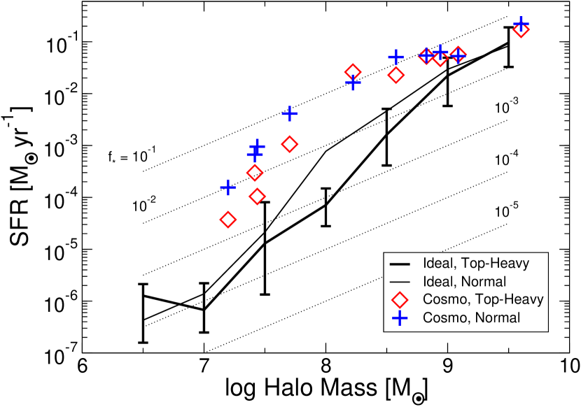
Figure 1.— The mean of the time-averaged star formation rates (SFR) for idealized halos. The thin and thick lines correspond to runs with a normal ($N_{\gamma}=2,600$) and top-heavy ($N_{\gamma}=26,000$) IMF, respectively. The error bars show the minimum and maximum values at each halo mass. The average SFR for cosmological halos with a top-heavy (normal) IMF are represented with diamonds (plus signs). The dotted lines show the SFR for a constant star formation efficiency, $f_{\star}=M_{\star}/M_{\rm{gas}}$, for $f_{b}$ = 0.1 and lasting for 100 Myr.

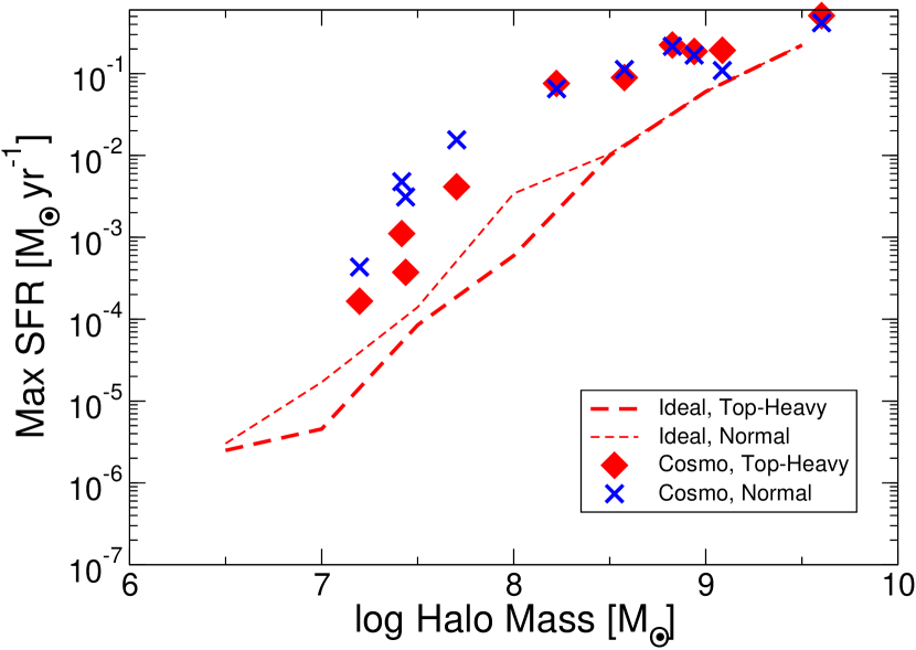
Figure 2.— The maximum SFR for idealized halos with a normal (thin dashed) and top-heavy IMF (thick dashed) and cosmological halos with a normal (crosses) and top-heavy IMF (diamonds).

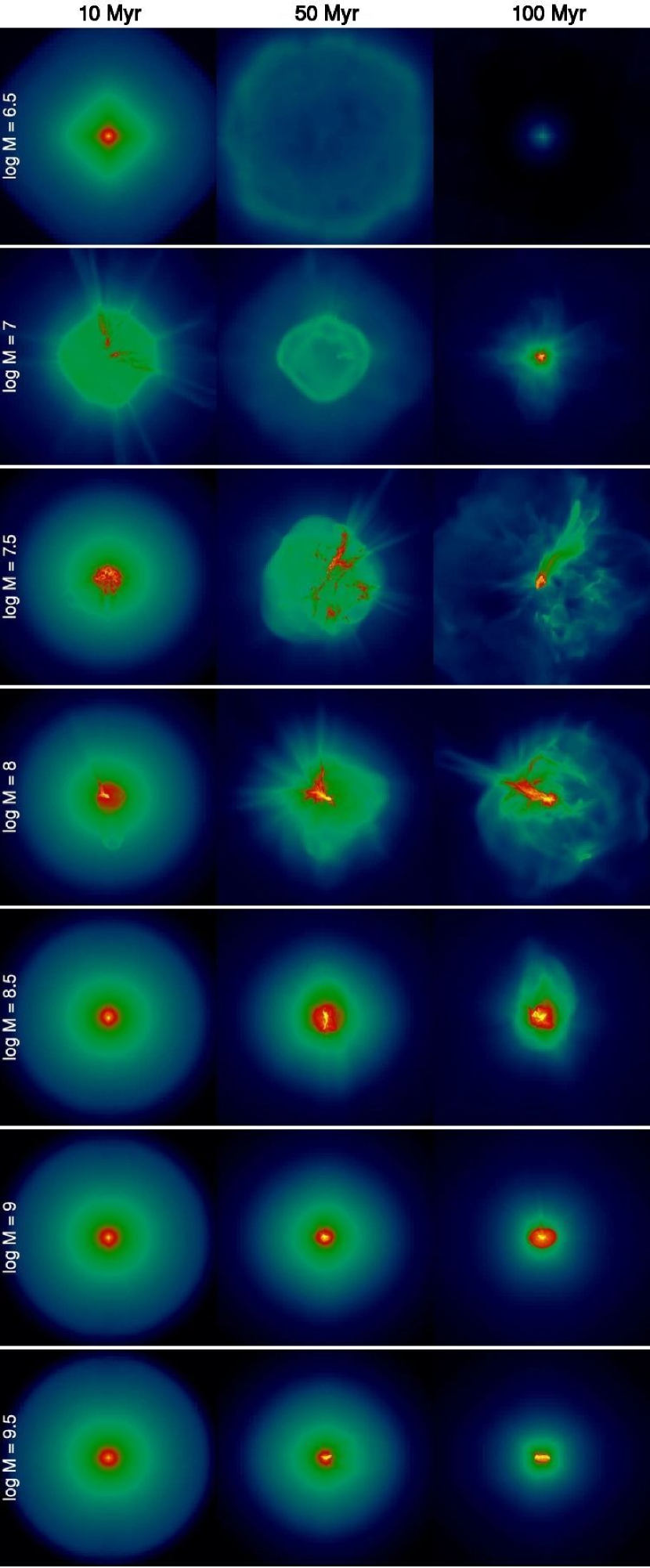
Figure 3.— Gas density projections, weighted by density squared for idealized halos. The field of view is 2$r_{\rm{vir}}$. The colormap spans 5 orders of magnitude from $10^{-3}$ to $10^{2}$ cm^-3.

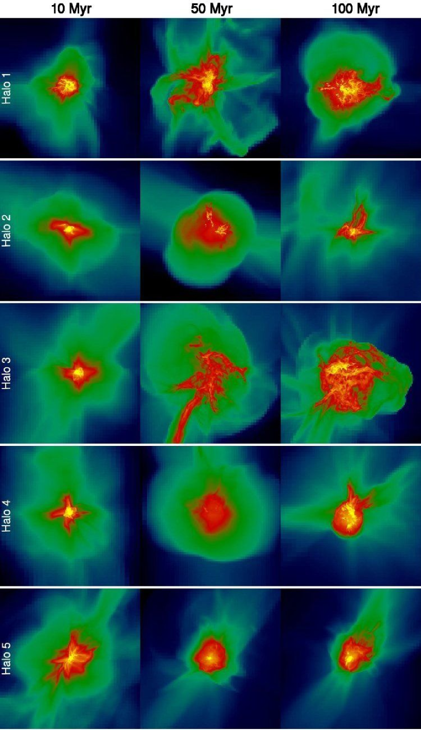
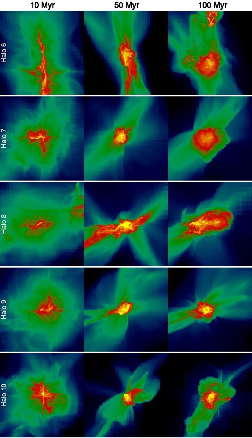
Figure 4.— Gas density projections, weighted by density squared for cosmological halos. Halos 1–10 have $\log_{10}({M_{\rm{vir}}})$ = 7.2, 7.4, 7.4, 7.7, 8.2, 8.6, 8.8, 8.9, 9.1, and 9.6. The field of view is 2$r_{\rm{vir}}$. The color scaling is the same as Figure 3.

3.1.1 Star Formation Rates

The escape fraction of UV radiation from halo is primarily dependent on the strength of the intrinsic ionizing luminosity and how it propagates through the gas into the IGM. The halos undergo an initial collapse and ensuing starburst. Afterwards star formation is self-regulated by radiative and supernovae feedback. We find that most of the UV radiation escapes during the most intense episodes of star formation, thus an important quantity to investigate is the maximum SFR of the halo, as well as the average. We plot the time-averaged and maximum SFR of the idealized and cosmological halos with a top-heavy and normal IMF in Figures 1 and 2, respectively. We also plot SFRs if a constant star formation efficiency, $f_{\star}=M_{\star}/M_{\rm{gas}}$, is assumed for a baryon mass fraction of 0.1 and a starburst lasting for 100 Myr.

The maximum SFRs are anywhere between 2–10 times the average SFR. The error bars show variances up to an order of magnitude in the star formation for a given halo mass in the idealized runs. For halos with ${M_{\rm{vir}}}>10^{7}{M_{\odot}}$, SFRs steadily increase as SFR $\propto{M_{\rm{vir}}}^{\alpha}$ with $\alpha\sim 2$. Idealized halos with $M_{\rm{vir}}$ = $10^{6.5}$ and $10^{7}$ $M_{\odot}$ have similar SFRs because they experience only one episode of star formation that blows away most of the gas in the halo, quenching any further star formation. In a more realistic cosmological setup, these outflows only delay later star formation because the gas reservoir can be replenished through gas accretion from filaments and mergers (Wise & Abel, 2008a). This accretion causes the SFRs to be higher up to a factor of 100 in cosmological halos up to ${M_{\rm{vir}}}=10^{8.5}{M_{\odot}}$, which can be seen in Figures 1 and 2. Above this halo mass, SFRs interestingly level off at $\sim$0.1 $M_{\odot}$ yr^-1, corresponding to an average star formation efficiency $f_{\star}=0.05-0.1$.

With a normal IMF, average and maximum SFRs in cosmological halos with ${M_{\rm{vir}}}\leq 10^{8}{M_{\odot}}$ increase by an order of magnitude. In these halos, outflows generated by radiative feedback is the main force in regulating SFRs. Therefore one expects less self-regulation of star formation, and thus higher SFRs, with a normal IMF when compared to a top-heavy one. In more massive halos, only outflows generated by SN explosions can escape from the potential well. Hence decreasing the specific stellar luminosity does not significantly affect the gas mass inside the halo, leading to similar SFRs in the top-heavy and normal IMF runs.

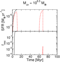
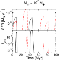
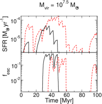
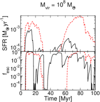
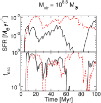
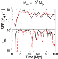
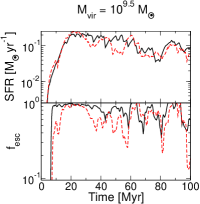
Figure 5.— Star formation rates (top panels) and UV escape fractions (bottom panels) for the idealized halo setup with $N_{\gamma}=26,000$ (solid) and 2,600 (dashed). The data are from models with ($f_{b}$, $\lambda$, $f_{\rm{turb}}$) = (0.1, 0.04, 0.25).

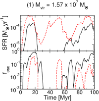
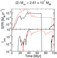
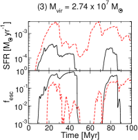
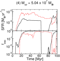
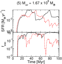
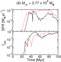
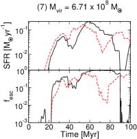
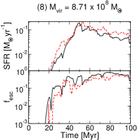
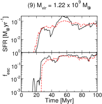
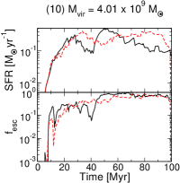
Figure 6.— Same as Figure 5 but for cosmological halos. The halo numbers are labeled in parentheses.

3.1.2 Stellar Feedback

In the dwarf galaxies that we consider, stellar feedback from H II regions and SN explosions creates galactic outflows that expel significant amounts of gas from the halo. Our simulations capture the formation of a D-type ionization front that accelerates matter up to 35  km s^-1 (e.g. Franco et al., 1990; Whalen et al., 2004; Kitayama et al., 2004; Abel et al., 2007), which is greater than the escape velocities of halos with ${M_{\rm{vir}}}\lower 3.00003pt\hbox{$\,\buildrel<\over{\sim}\,$}10^{8.5}{M_{\odot}}$ at redshift 8. Above this mass, SNe feedback, which generates outflows up to $\sim$300 km s^-1, becomes the dominant force in expelling gas. Feedback strongly affects the gas structures within the dwarf galaxies, which we illustrate in density-squared projections of gas density of idealized and cosmological halos in Figures 3 and 4 at 10, 50, and 100 Myr after the initial starburst.

The transition from complete gas “blow-out” to “blow-away” is apparent in the idealized halos (Fig. 3) at $M\lower 3.00003pt\hbox{$\,\buildrel>\over{\sim}\,$}10^{8.5}{M_{\odot}}$. In halos with ${M_{\rm{vir}}}=10^{6.5-7}{M_{\odot}}$, the D-type front is unbound from the halo and expels most of the gas with it. Only a small fraction returns to the halo center after 100 Myr. In halos with ${M_{\rm{vir}}}=10^{7.5-8}{M_{\odot}}$, the blow-out becomes less effective at completely evacuating the halo because of the deeper potential well. As stated before when the D-type front velocity is less than the escape velocity of the halo, radiative feedback cannot create unbound galactic outflows. Nevertheless, it still plays a key role in shaping the small-scale ($l\lower 3.00003pt\hbox{$\,\buildrel<\over{\sim}\,$}100$ pc) variations in the ISM density and temperatures.

The cosmological halos provide a more realistic environment and halo setup—inflows from filaments, minor mergers, turbulent velocity fields, an evolving DM potential—in studying the effects of star formation and feedback. Despite the more realistic gas inflows in such halos, we find a similar transition from blow-out to blow-away at ${M_{\rm{vir}}}=10^{8.5}{M_{\odot}}$. The halos with ${M_{\rm{vir}}}<10^{8}{M_{\odot}}$ are not evacuated like their idealized counterparts because of additional gas accretion from adjacent filamentary structures and minor halo mergers . In response, star formation is self-regulating, in which the stellar radiation reduces the amount of cool and dense gas available for star formation. In the least massive halos, star formation ceases for tens of millions of years as the relic H II region cools and re-condensed. We further discuss star formation rates in §3.1.3–3.1.4.

Above $10^{8}$ $M_{\odot}$, radiative feedback does not destroy all of the density enhancements, in particular one centred in the halo center, and stars continue forming in the presence of nearby star clusters. The infalling subhalo (${M_{\rm{vir}}}\sim 10^{7}{M_{\odot}}$) in Halo 6 at $t$ = 100 Myr provides an interesting contrast in the halo mass dependence of radiative feedback, where the main halo is centrally concentrated while the subhalo is being blown apart by radiative feedback. In these more massive halos, star formation is still self-regulated but not suppressed as there is a persistent cold gas reservoir available for star formation, as seen in the evolution of gas density in the right column of Figure 4.

3.1.3 Star Formation History of Idealized Halos

We plot the star formation histories of the idealized control halos ($f_{b}$ = 0.1, $\lambda$ = 0.04, $f_{\rm{turb}}$ = 0.25) in the top panels of Figure 5. Star formation in halo masses below $10^{8}$$M_{\odot}$ is episodic. This occurs when radiation driven stellar outflows expel most of the gas from the halo, quenching star formation. Once the gas is no longer irradiated, it can cool and fallback into the halo center, forming stars once again. This occurs up to 5 times in these halos in the 100 Myr, more often in more massive halos.

When halo masses increase to between $10^{7.5}$ and $10^{8.5}$ $M_{\odot}$, star formation continues in the presence of galactic outflows; however it soon halts once the cool gas reservoir in the halo is depleted. In Figure 5, one sees in halos with these masses experience at least one period of quiescence, where a substantial fraction of gas cannot form star-forming molecular clouds because it is contained in outflows. Similar to the lower-mass halos, star formation recommences after gas falls back into the halo.

Above $10^{9}$$M_{\odot}$, the bursting behavior of star formation is entirely eliminated. The potential well of the halo has become deep enough ($V_{c}>35$  km s^-1) to contain any outflows created by over-pressurized H II regions. The transition circular velocity from baryon “blow-out” to “blow-away” is similar to the velocities generated in D-type ionization fronts. Furthermore, unlike the lower mass halos, the roughly constant SFRs are approximately the same between the high- and low-luminosity models at $5\times 10^{-2}$ and $10^{-1}$ $M_{\odot}$ yr^-1 for $M_{vir}=10^{9}$ and $10^{9.5}{M_{\odot}}$, respectively.

Thin disk formation is absent in halos that experience baryon blowout because the outward motions created in H II regions disrupt any global organized rotation. In halos with ${M_{\rm{vir}}}>10^{9}{M_{\odot}}$, the majority of gas is retained within the halo, which then settles into a thin disk. We caution that is probably not strong evidence for a transition from a globally turbulent ISM to disk formation because of our idealized setup of solid-body rotation. We can better investigate any morphological trends in cosmological halos that are described in the following section.

3.1.4 Star Formation History of Cosmological Halos

We show the star formation histories for the 10 selected cosmological halos in the top panels of Figure 6. The SFR in cosmological halos is less episodic than the idealized halos because the cosmological gas accretion replenishes the galaxy, balancing the effect of any blow-away. Nevertheless star formation is still self-regulated, which can be seen in the SFR being suppressed up to an order of magnitude after a local maximum in SFR. Afterwards the SFR recovers again because of the reduced radiative feedback. This modulation occurs in all cosmological halos studied here.

In lower mass halos with ${M_{\rm{vir}}}<10^{8}{M_{\odot}}$ with a top-heavy IMF, star formation is still completely eliminated for 10–20 Myr. This does not occur in the same halos with a normal IMF because the galactic outflows are weaker, making it easier for the cosmological accretion to penetrate through the outflows. Hence star formation is continuous in these cases. Similar to the ${M_{\rm{vir}}}>10^{9}{M_{\odot}}$ idealized halos, SFRs are not significantly affected by a lower specific stellar luminosity in cosmological halos with ${M_{\rm{vir}}}>10^{8}{M_{\odot}}$. There are some deviations by a factor of a few in the evolution of the SFR in these halos, but the time-averaged rates are largely unaffected. One clear example of this behavior occurs in Halo 6 (${M_{\rm{vir}}}=3.8\times 10^{8}{M_{\odot}}$) at t = 70 Myr. In the top-heavy IMF case, radiative feedback from the initial burst subdues star formation from t = 50–80 Myr by a factor of 5. In contrast, the feedback from a normal IMF does not suppress star formation, which continues at a rate of $\sim$$10^{-1}{M_{\odot}}~{}\rm{yr}^{-1}$. Furthermore, galactic disk formation, which is seen in isolated halos with ${M_{\rm{vir}}}\geq 10^{9}{M_{\odot}}$, is absent in all of the cosmological cases.

3.1.5 Comparison to Previous Work

The SFRs in the ${M_{\rm{vir}}}=10^{9.5}{M_{\odot}}$ halos are $\sim$$10^{-1}$ $M_{\odot}$ yr^-1 and are similar to the least massive ($M_{\rm{vir}}$ $\sim$ $10^{10}$$M_{\odot}$) halos in GKC08. However for a direct comparison of SFRs and escape fractions, we must either use the simulations with $N_{\gamma}$ = 2,600 or consider the SFRs from top-heavy IMF simulations as effectively 10 times greater. Fujita et al. (2003) characterizes star formation with a star formation efficiency $f_{\star}=M_{\star}/M_{d}$, where $M_{d}$ is the total gas disk mass. If we equate the total gas mass in our halos to the disk mass of Fujita et al., our ${M_{\rm{vir}}}=10^{9}{M_{\odot}}$ idealized halos are comparable to their high-redshift $M_{d}=10^{8}{M_{\odot}}$ models with $f_{\star}=0.06$.

3.2. UV Escape Fraction

A fraction of the stellar radiation emitted from the stars described in the previous section escape into the IGM. This quantity is an essential parameter in both semi-analytical reionization models (e.g. Cen, 2003a, b; Wyithe & Loeb, 2003a; Haiman & Holder, 2003) and N-body reionization simulations (e.g. Ciardi et al., 2003; Sokasian et al., 2003; Iliev et al., 2006; Trac & Cen, 2007). First we discuss the trends of $f_{\rm esc}$ with halo mass of the idealized halos. We then describe the behavior of $f_{\rm esc}$ with respect to important physical parameters: turbulent energy, halo spin parameter, and baryon mass fraction. Next we discuss the results of $f_{\rm esc}$ in halos that have been extracted from cosmological simulations. We end this section discussing anisotropic H II regions and its relevance in the UV escape fraction.

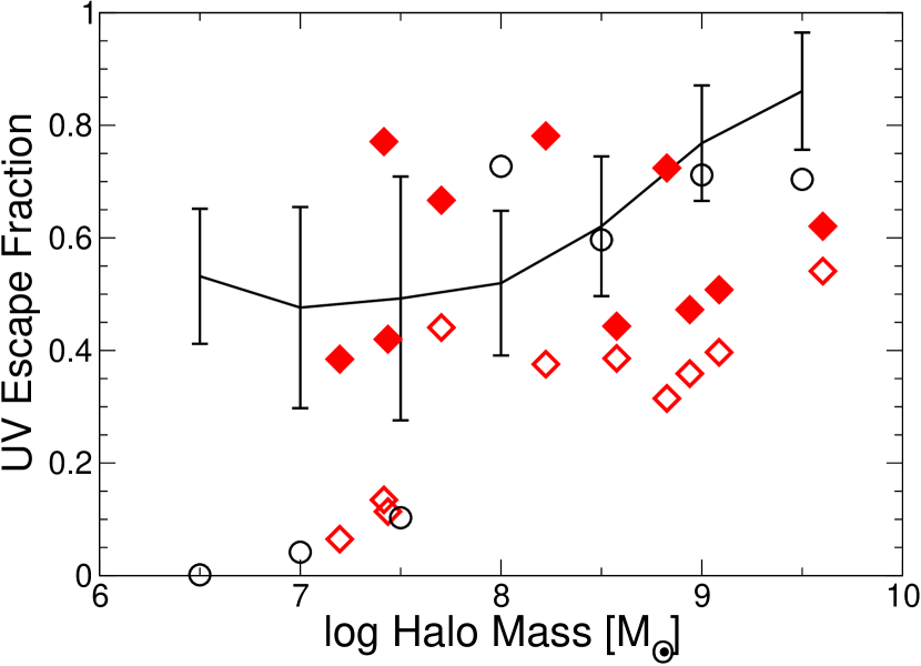
Figure 7.— Escape fraction of ionizing photons from idealized halos with a top-heavy IMF (solid line) and normal IMF (circles) and cosmological halos with a top-heavy IMF (filled diamonds) and normal IMF (open diamonds) as a function of halo mass.

3.2.1 Idealized halos

We plot the evolution of $f_{\rm esc}$ of the idealized halos in the bottom panels of Figure 5. Before presenting our results of $f_{\rm esc}$ in these halos, we would like to warn that one should not take the values of $f_{\rm esc}$ as absolute because of the lack of gas accretion and adjacent filamentary structures. Nevertheless it is appropriate to study the temporal variations and changes with physical parameters.

In halos with ${M_{\rm{vir}}}\leq 10^{7}{M_{\odot}}$, $f_{\rm esc}$ behaves in a predictable manner, in which star formation is confined within a small region and happens in bursts. Thus most of the escaping radiation experiences similar gaseous structures when propagating outwards. In the bursts, the $f_{\rm esc}$ quickly increases when the H II region breaks out from the halo, which can take up 10 Myr after the starburst starts. The escape fraction peaks when the SFR is at its maximum and varies anywhere from $10^{-3}$ to unity, depending on the column density of the surrounding medium.

In more massive halos, the escape fraction is highly dependent on preceding star formation and its effect on the gas structure. For example in halos with ${M_{\rm{vir}}}$ = $10^{7.5}$ – $10^{8.5}$ $M_{\odot}$, SFRs that differ by an order of magnitude can produce similar values of $f_{\rm esc}$. In the initial starburst, the radiation needs to escape through a relatively smooth $r^{-2}$ density profile and $f_{\rm esc}\geq 0.5$. Then conditions quickly erode from this smooth initial state to a turbulent multi-phase ISM because of both radiative cooling and stellar feedback. Now radiation must escape through a clumpy and turbulent ISM, whose porosity can increase $f_{\rm esc}$ for a given luminosity or SFR (Clarke & Oey, 2002).

Generally only radiation from the strongest starbursts can escape, whereas during suppressed periods of star formation very little ($f_{\rm esc}<0.01$) radiation escapes. As SFRs become more consistent in halos with ${M_{\rm{vir}}}>10^{9}{M_{\odot}}$, the escape fraction varies between 0.1 and 1.0 with less variation than the lower mass halos. In addition, we find that radiation from stars that form on the outskirts of the thin disk have a higher escape fraction than stars that are deeply embedded within the galaxy, which is similar to the results of GKC08.

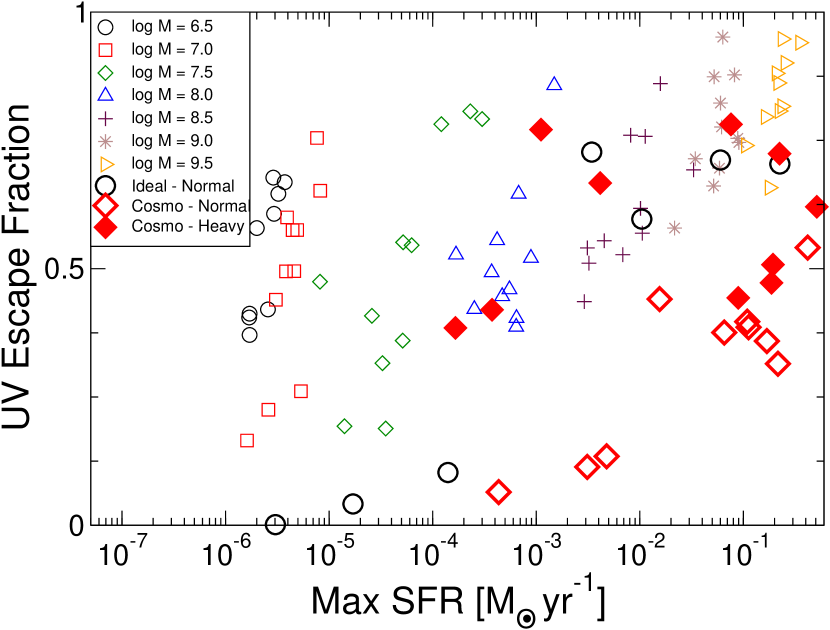
Figure 8.— Escape fraction of ionizing photons as a function of maximum star formation rate from all simulated halos, showing a strong dependence for a given halo mass. Idealized halos with equal halo masses are plotted with the same symbols. Idealized halos with a normal IMF are plotted as large circles ranging from $10^{6.5}$ to $10^{9.5}{M_{\odot}}$ from left to right. Cosmological halos with a top-heavy and normal IMF are plotted as filled and open diamonds, respectively.

In Figure 7, we plot the average UV escape fraction as a function of halo mass, where the error bars indicate the standard deviation of $f_{\rm esc}$ over the 11 models for each halo mass. Halos with ${M_{\rm{vir}}}\leq 10^{8}{M_{\odot}}$ have $f_{\rm esc}\sim 0.5\pm 0.2$. For a normal IMF in these low-mass halos, $f_{\rm esc}$ drops to values below 0.1. Escape fractions steadily increase with halo mass to $\sim$0.8 above this mass for both top-heavy and normal IMFs.

As seen in Figure 5, $f_{\rm esc}$ is highest when the SFR is at its maximum, max(SFR). To depict this strong dependence on the strength of the starburst, we show $f_{\rm esc}$ for every simulated halo as a function of max(SFR) in Figure 8, grouped by halo mass. For instance in the ${M_{\rm{vir}}}=10^{7.5}{M_{\odot}}$ halos, $f_{\rm esc}$ increases from 0.2 to 0.8 when max(SFR) is higher by an order of magnitude. We have also plotted the idealized halos with a normal IMF as large open circles.

3.2.2 Dependence on halo parameters

Although the absolute values of $f_{\rm esc}$ in idealized halos are inaccurate for reasons discussed in the previous section, we can utilize the trends with physical halo parameters—baryon mass fraction, spin parameter, and turbulent energy—to estimate $f_{\rm esc}$ in cosmological halos other than the ones studied in this paper. For example, Wise & Abel (2008a) found that the first stars lowered the baryon mass fraction to $\leq 0.1$, but the halos from our adiabatic cosmological simulations have $f_{b}\sim 0.13$. We can then use the trends in $f_{\rm esc}$ with respect to $f_{b}$ to estimate the effects of neglected processes on the escape fraction. We show these trends for all idealized halos in Figure 9.

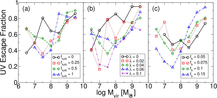
Figure 9.— UV escape fraction versus halo mass plotted for varying values of (a) turbulent energy, (b) spin parameter, and (c) baryon mass fraction.

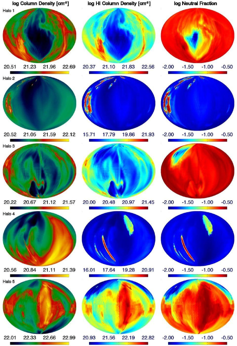
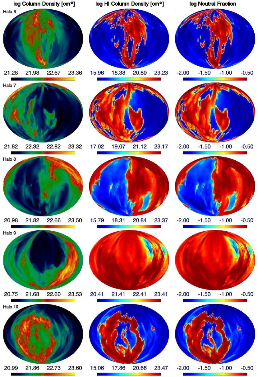
Figure 10.— Full-sky maps of total column density (first and fourth columns), H I column density (second and fifth columns), and mass-weighted neutral hydrogen fraction (third and sixth columns) 50 Myr after the initial starburst in the cosmological halos. Halos 1–10 have $\log_{10}({M_{\rm{vir}}})$ = 7.2, 7.4, 7.4, 7.7, 8.2, 8.6, 8.8, 8.9, 9.1, and 9.6. The observer is at the center of mass of the halo, and the quantities shown out to the virial radius. The colormaps for column density are unique for each halo; however the electron fraction colormaps have a fixed range of 0.01–0.3. Halos 2 and 4 are almost completely ionized, and halos 6, 7, and 10 represent clear examples of anisotropic H II regions, which escape from the halo where the column density is lowest.

Turbulent energy— Initial turbulent energy should be unimportant in the more massive halos as radiative and SN feedback continuously alters the ISM and further stirs turbulence (e.g. Scalo & Elmegreen, 2004), perhaps overpowering any pre-existing turbulence. There are no consistent trends with turbulent energy between $10^{6.5}$ – $10^{9.5}$ $M_{\odot}$. However in the ${M_{\rm{vir}}}=10^{7.5}{M_{\odot}}$ halos, the $f_{turb}=0$ case has $f_{\rm esc}=0.8$ that is up to twice the escape fraction of the other halos. This occurs because turbulent flows are not present to disrupt the initial halo collapse, resulting in a stronger initial starburst and escalating the average escape fraction. The $f_{turb}=0$ case with ${M_{\rm{vir}}}=10^{8}{M_{\odot}}$ is only marginally higher than the other halos by $\sim$25%. This anomaly is not present in other halo masses.

Spin parameter— Similar to the lack of apparent trends with turbulent energy, spin parameter has little effect on the UV escape fraction. One exception is the non-spinning case above $10^{7}$ $M_{\odot}$, having the largest escape fraction. This arises from a strong central collapse without being rotationally supporting, resulting in a stronger initial starburst. However this scenario is improbable in reality because of abundant cosmological tidal torques (Hoyle, 1949; Peebles, 1969), culminating in a log-normal spin parameter distribution that has a mean value of 0.042 (e.g. Barnes & Efstathiou, 1987; Bullock et al., 2001a).

Baryon mass fraction— Out of the three physical parameters studied, the baryon mass fraction plays the largest role in regulating star formation and the escaping radiation. In halos with ${M_{\rm{vir}}}<10^{8}{M_{\odot}}$, the $f_{b}=0.15$ case has $f_{\rm esc}$ lower than the other gas fractions by a factor of 2. The increased neutral column density that the radiation must transverse before breaking out of the halo causes the decrease. Interestingly above $10^{8}$ $M_{\odot}$, this trend reverses, and higher gas fractions result in larger escape fractions. Here the gas-rich halos can sustain a higher SFR, and the corresponding higher ionizing luminosity can escape the halo more freely than in the gas-poor ($f_{b}\leq 0.1$) halos, even though the radiation has a larger column to ionize.

3.2.3 Cosmological halos

The star-forming cosmological halos represent a more realistic setup of high-redshift, starburst dwarf galaxies, necessary to calculate a robust value of the UV escape fraction. In the lower panels of Figure 6, we show the escape fraction of the cosmological halos as a function of time. During the first starburst that originates from the initial halo collapse, instantaneous $f_{\rm esc}$ values widely vary from less than 10^-3 up to nearly unity. Most importantly the escape fraction depends on the current star formation and any of its time variations. As seen in Figure 6 the variations in SFR corresponds to variations in $f_{\rm esc}$ on similar timescales, on order of a dynamical timescale of a molecular cloud, $\sim$1–3 Myr. In halos 2 and 4, a constant SFR exists for 30 Myr in the top-heavy IMF case. The cumulative luminosity from this stellar cluster gradually ionizes the IGM and photo-evaporates most clumpy material. Eventually the escape fraction approaches unity after $\sim$10 Myr of irradiation.

As with the idealized halos, the escape fraction is dependent on the previous star formation history, which can photo-evaporate dense, clumpy material in the halo. Imagine two equal-mass stellar clusters, forming in the same neighborhood. The one that forms first will pre-ionize the ISM in some fraction of solid angle, allowing the radiation from the second cluster to escape into the IGM more easily and further raising the escape fraction.

We compare $f_{\rm esc}$ from cosmological halos with their idealized counterparts in Figures 7 and 8 with respect to virial mass and maximum SFR, respectively. The halos that host a top-heavy IMF have escape fractions within the scatter of the idealized halo, even though adjacent filamentary structures can absorb most of the radiation in their line of sight. Their $f_{\rm esc}$ values range from 0.4 to 0.8. We also find that $f_{\rm esc}$ at half and twice the virial radius are within 10% of the value at $r_{\rm{vir}}$, similar to GKC08, because the nearby clumps and adjacent filaments do not contribute a significant solid angle for absorption.

A normal IMF lowers the escape fraction by $\Delta(f_{\rm esc})$ = 0.05–0.4. It is interesting that $f_{\rm esc}$ is approximately 0.4 with a normal IMF over 2 orders of magnitude in halo mass and maximum SFR, starting with ${M_{\rm{vir}}}=10^{7.5}{M_{\odot}}$. Halos below this mass threshold (i.e. efficient atomic cooling) are affected considerably by a normal IMF, where $f_{\rm esc}$ drops by a factor of a few to values of 0.05–0.1.

3.2.4 Anisotropic H II Regions

In our radiation hydrodynamics simulations, radiative feedback greatly affects the gas dynamics inside the halos. Any UV radiation will first escape from the halo in the direction with the least H I column density. This creates anisotropic H II regions with the radiation preferentially escaping through these channels. Any adjacent filamentary structures, which provide the halo with a cold, dense flow (Nagai et al., 2003; Kereš et al., 2005; Dekel & Birnboim, 2006; Wise & Abel, 2007a), and cold and clumpy ISM are the major components in absorbing outgoing radiation.

We create full-sky maps of total and H I column density and mass-averaged neutral fractions of the cosmological halos with a top-heavy IMF 50 Myr after the initial starburst in Figure 10. These maps are created by casting adaptive rays (Abel & Wandelt, 2002) from the center of mass of the halo to the virial radius. Each ray tracks the total and neutral column density along its path. We then reconstruct a full-sky map of these quantities using the spatial information contained in the HEALPix formalism. The ionized regions (blue) match well with the areas with the lowest column density (black and dark blue). The transitions from neutral to ionized in these maps are abrupt, depicting how any neutral blobs can completely absorb the radiation in its solid angle. However, in the solid angles where the ionized fraction is close to unity, almost all of the radiation can escape, i.e. $f_{\rm esc}=1$ in those directions. The simulations of RS06, RS07, and GKC08 also see the majority of solid angles having $f_{\rm esc}$ equal to either unity or zero.

At $t=50$ Myr, halos 1 and 3 are in a quiescent state, and the previously ionized ISM and IGM is recombining. The relic H II region are still visible in the full-sky maps. Here the transition from ionized and neutral regions are gradual because of the longer recombination times in diffuse gas. Halos 2 and 4 have been almost completely ionized at the end of a starburst. Notice the cometary tails created by photo-ionization of a clumpy medium (e.g. Susa & Umemura, 2006; Whalen et al., 2008) at the northern section in halo 2 and the middle-bottom region in halo 4. In the former case, the neutral shadow, pointing southwest, of the small overdensities are clear in the neutral fraction map. In halos 5–10, stellar radiation escapes through a large fraction ($>25\%$) of solid angle, which correspond to the path of least neutral column density.

3.2.5 Comparison to Previous Work

Clearly these escape fractions contradict the results from GKC08, where their lowest mass halos with ${M_{\rm{vir}}}\sim 10^{10}{M_{\odot}}$ have $f_{\rm esc}=10^{-5}-10^{-2}$ at $z=3-5$. From the examples given there, the stars are born within a galactic disk, unlike our simulations, which could be causing their smaller escape fractions. In §4, we further discuss possible causes of this discrepancy. Although our galaxies are smaller by a mass factor of $>$100 than the ones simulated in RS06 and RS07, it is worth reiterating that they find $f_{\rm esc}=0.01-0.1$ at redshift 3. Both groups also find that $f_{\rm esc}$ can significantly vary from galaxy to galaxy and in different lines of sight to each galaxy. Escape fractions in Fujita et al. (2003) exceed 0.2 in their high-redshift dwarf galaxies if the starbursts are intense, i.e. their $f_{\star}\geq 0.06$ models, similar to our $f_{\rm esc}$ values in the most massive halos.

4. Discussion

The fraction of ionizing radiation that escapes high-redshift galaxies is an important value to quantify in order to characterize cosmological reionization. In this section, we first discuss the differences and similarities, along with their respective causes, between our results and previous work. Next we discuss any implications and agreements with semi-analytic reionization models. We last elaborate on possible influences from neglected physical processes.

4.1. Possible Physical and Computational Dependencies

Our results suggest that $f_{\rm esc}$ is higher than 0.1 in such galaxies, but we must first understand why our $f_{\rm esc}$ values differ from the more massive galaxies presented in the simulations of Razoumov & Sommer-Larsen (2006, 2007) and Gnedin et al. (2008). Below we discuss five possible causes.

Galaxy morphology and environment— The galaxies simulated here exhibit an irregular morphology and did not form a rotationally-supported disk, whereas the simulations of RS06, RS07, and GKC08 all studied disk galaxies. As mentioned in Fujita et al. (2003), a turbulent and clumpy ISM may allow for radiation to escape more easily into the IGM. Compared to a disk configuration, there are more low-density escape routes, i.e. porosity, for the radiation because of the clumpy nature of the gas (Clarke & Oey, 2002). Furthermore, the stellar orbits are not confined within a disk and can reach the outskirts of the galaxy at apocenter, where gas densities are much lower than the galactic center and ionizing radiation can escape into the IGM at a much greater rate. Perhaps this irregular morphology is only initially present in dwarf galaxies because radiative feedback shifts the angular momentum distribution to higher values (Wise & Abel, 2008a). A fraction of this material will return to the galaxy and aid in disk formation in higher mass galaxies, such as the ones studied in RS06, RS07, and GKC08. Furthermore in rare halos, the intersecting filaments tend to be dense and thin, where a halo with equal mass at lower redshift would be contained in a large filament (Ocvirk et al., 2008). This redshift dependency on halo environment could affect $f_{\rm esc}$ at $r>r_{\rm vir}$, but should not be apparent at $r_{\rm{vir}}$.

Galactic mass— GKC08 find that $f_{\rm esc}$ increases as much as 3 orders of magnitude from a halo mass of $10^{10}$ to $10^{11}$$M_{\odot}$. The cold H I disk in their lower mass galaxies tend to be more vertically extended, which brings about this precipitous drop. If this trend continues to lower masses, the values of $f_{\rm esc}$ would be negligible in our galaxies, but we see no such continuation. Our results suggest that the radiative feedback in dwarf galaxies with $V_{c}\lower 3.00003pt\hbox{$\,\buildrel<\over{\sim}\,$}35{~{}{\rm km~{}s^{-1}}}$ have a profound impact on the ISM by driving outflows and preventing any disk formation, increasing $f_{\rm esc}$. Perhaps this circular velocity is a critical turning point below which $f_{\rm esc}$ is large ($>0.1$) because of dynamical effects from radiative feedback. In more massive galaxies, SN feedback provides the main impetus for driving outflows.

Star formation rates— One can argue that our simulations only capture the initial collapse and an artificially strong starburst in high-redshift galaxies; however, after $\sim$20 Myr of star formation, this collapse is reversed by stellar feedback and SFRs stabilize. In addition our most massive galaxy (${M_{\rm{vir}}}=4\times 10^{9}{M_{\odot}}$) has an average SFR of 0.2 $M_{\odot}$ yr^-1, which is comparable to the SFRs found in the ${M_{\rm{vir}}}\sim 10^{10}{M_{\odot}}$ galaxies in GKC08. The star formation efficiencies ($M_{\star}/M_{\rm{gas}}$) of our galaxies range from 5–10%, also agreeing with previous galaxy formation simulations. Hence we do not think our treatment of star formation affects the SFRs and resulting UV escape fraction.

Stellar IMF— We experimented with both normal ($N_{\gamma}=2,600$) and top-heavy ($N_{\gamma}=26,000$) IMFs and found that a normal IMF causes $f_{\rm esc}$ values to be lower by 10–75%. The differences in how the gas and ensuing star formation reacts to radiative feedback most likely causes this spread. The normal IMF is similar to the ones used in all previously quoted theoretical works, and thus we do not expect our choice in IMF to cause our high UV escape fractions. One minor shortcoming of our simulations is that we keep the SN feedback strength equal in our normal and top-heavy IMFs. Although this helps us localize the cause of any changes to a different specific luminosity, the strength of SN feedback should also affect the gas distribution, SFR, and $f_{\rm esc}$.

Resolution— We can afford a spatial resolution of $\sim$0.1 physical pc in all of our simulations. However in larger galaxies, it becomes increasingly difficult to maintain this resolution, especially in cosmological simulations. The highest resolution simulation in RS06 and RS07 use a gravitational softening length of 330 $h^{-1}$ pc, and their radiative transfer grid is refined so that 10 particles occupy each cell. GKC08 use AMR simulations with a maximum resolution of 50 physical pc. Fujita et al. (2003) have a fixed resolution of 0.28 pc in their $z=8,M_{d}=10^{8}{M_{\odot}}$ simulation, similar to our resolution. The $f_{\rm esc}$ values of our simulations and Fujita et al. are in agreement. Regular and giant molecular clouds have radii of 2–20 and 10–60 pc (see Mac Low & Klessen, 2004, for a review), respectively, and are usually accounted with subgrid physics in cosmological simulations. However our simulations capture the turbulent and clumpy nature of the ISM, while resolving such molecular clouds. As discussed before, the turbulent ISM and its porosity may play a key role in allowing radiation to escape (Clarke & Oey, 2002). In addition, high-resolution simulations with radiative transfer can model the fragmentation of ionization fronts (e.g. Fujita et al., 2003; Whalen & Norman, 2008), which can further assist in boosting UV escape fractions.

4.2. Impact on reionization models

In reionization models, whether it be based on Press-Schetcher formalism or N-body simulations, the product ${f_{\rm esc}^{\star}}\equiv f_{\star}\times{f_{\rm esc}}$ ultimately dictates the absolute number of photons that escape from each halo into the IGM. When calibrating these models against WMAP observations (Spergel et al., 2007; Komatsu et al., 2008) and Ly$\alpha$ transmission from $z\sim 6$ quasars (e.g. Bolton & Haehnelt, 2007; Srbinovsky & Wyithe, 2008), the values of $\geq 0.01$ are usually required. Recently, Srbinovsky & Wyithe found that $f_{\rm esc}$ must lie within the range 0.1–0.25 with a best-fit of $f_{\star}=0.11$ if all halos with masses $\lower 3.00003pt\hbox{$\,\buildrel>\over{\sim}\,$}10^{9}{M_{\odot}}$ contribute to reionization. Furthermore, they conclude that even the smallest atomic line cooling halos (${M_{\rm{vir}}}\lower 3.00003pt\hbox{$\,\buildrel>\over{\sim}\,$}10^{8}{M_{\odot}}$) have ${f_{\rm esc}}\sim 0.05$. Our results support this scenario where low-luminosity galaxies are the main contributors to reionization.

We plot $f_{\rm esc}^{\star}$ from idealized and cosmological halos in Figure 11. We calculate $f_{\star}$ using the initial gas mass in halo at the initial time; thus we are overestimating $f_{\star}$ up to a factor of $\sim$1.5 because the halos experience mass accretion in the 100 Myr that we have simulated. Recall that none of the halos presented here undergo a major merger. In our least massive cosmological halos with ${M_{\rm{vir}}}\leq 3\times 10^{7}{M_{\odot}}$, $f_{\rm esc}^{\star}$ increases rapidly with respect to halo mass from $10^{-3}$ to $10^{-2}$ because atomic hydrogen line cooling becomes efficient in these halos. $f_{\rm esc}^{\star}$ is also an order of magnitude higher than the idealized cases. As discussed in §3.1.1, the additional gas accretion from filaments results in higher SFRs or equivalently $f_{\star}$. In atomic cooling halos (${T_{\rm{vir}}}>8000$ K), we find $f_{\rm esc}^{\star}$ to always be $\geq 0.01$, sufficiently high enough to meet the “critical” value to match reionization constraints, with an average of 0.033 and 0.026 for top-heavy and normal IMFs, respectively. When integrated over a luminosity function with a faint-end slope of –1.7 (e.g. Bouwens et al., 2007), the average of $f_{\rm esc}^{\star}$ in atomic cooling halos is 0.029 and 0.021 for top-heavy and normal IMFs, respectively. If we include all halos, this average drops to $4.1\times 10^{-3}$ because the low-mass halos are more abundant and cannot cool and form stars as efficiently.

In Figure 12, we show the behavior of $f_{\rm esc}^{\star}$ with halo mass in idealized halos grouped by halo parameters, similar to Figure 9. There is no apparent trends with respect to turbulent energy; however, halos with higher spin parameters result in smaller values of $f_{\rm esc}^{\star}$ in high mass halos that form a rotationally supported disk. The halos with $f_{b}=0.1$ have the highest values of $f_{\rm esc}^{\star}$, and gas-poor halos are consistently lower in all halo masses.

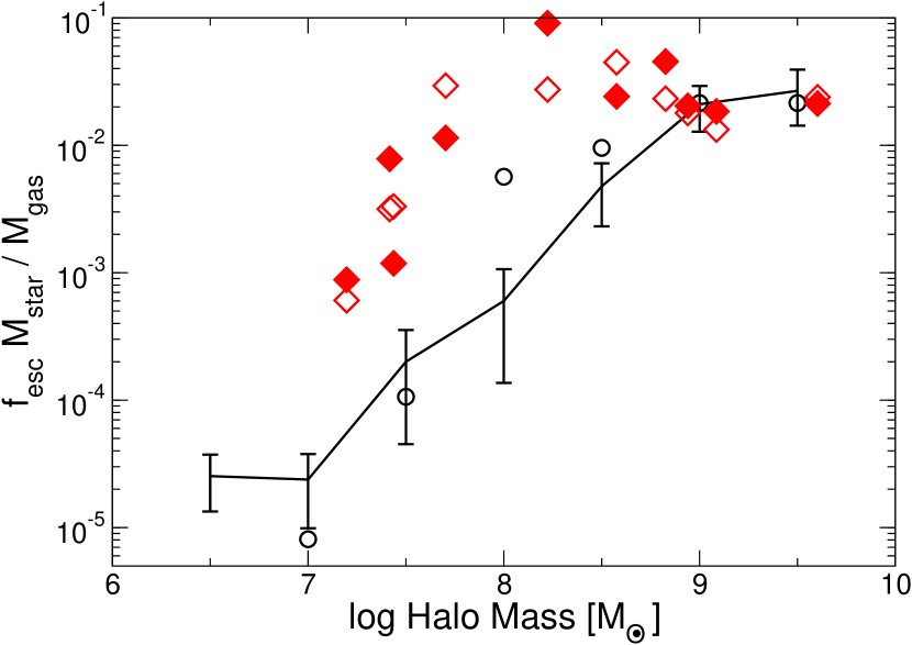
Figure 11.— The product of stellar mass fraction ($M_{\rm star}/M_{\rm gas}$) and escape fraction of ionizing photons ($f_{\rm esc}$) from idealized halos and cosmological halos with a top-heavy IMF (filled diamonds) and normal IMF (open diamonds) as a function of halo mass. Idealized halos with a normal IMF are plotted as large circles. This product is a key quantity in semi-analytical reionization models in determining the amount of escaping radiation per collapsed gas fraction.

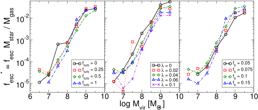
Figure 12.— Relative changes in the product of stellar mass fraction ($M_{\rm star}/M_{\rm gas}$) and escape fraction of ionizing photons ($f_{\rm esc}$) from all idealized models grouped by initial halo parameters: turbulent energy (left), spin parameter (middle), and baryon mass fraction (right) when compared to the “control halos” with ($f_{\rm turb},\lambda,f_{b}$) = (0.25, 0.04, 0.1).

4.3. Effects from the Ultraviolet Background

Our simulations accurately track the evolution of the H II regions and how they breakout into the IGM. Here we discuss an important process that was neglected in our simulations, external feedback from the UV background (UVB).

Our models sample halos that are primarily dependent on H₂ cooling (${T_{\rm{vir}}}\lower 3.00003pt\hbox{$\,\buildrel<\over{\sim}\,$}8000$ K) and atomic line cooling in more massive halos. Gas condensation in the lower mass H₂ cooling halos can be delayed by a H₂ dissociating UV (Lyman-Werner) background between 11.2 and 13.6 eV (Machacek et al., 2001; Wise & Abel, 2007b; O’Shea & Norman, 2008). The Lyman-Werner background thus increases cooling times in the centers of such halos. As a result, the minimum mass of a star-forming halo increases with the Lyman-Werner background intensity. This will not affect the global halo properties but may suppress the SFR in these halos. The Lyman-Werner background becomes less of an issue in atomic line cooling halos as Ly$\alpha$ cooling provides ample amounts of free electrons for H₂ cooling, and they become self-shielding to this radiation (Wise & Abel, 2008a).

We now consider any photo-heating from a hydrogen ionizing UVB, which can partially suppress gas accretion and thus star formation in dwarf galaxies (e.g. Efstathiou, 1992; Shapiro et al., 1994; Thoul & Weinberg, 1996). Here the Jeans “filtering mass” (Gnedin & Hui, 1998) accurately describes the minimum halo mass that can cool and collapse given an IGM thermal history (Gnedin, 2000; Wise & Abel, 2008b). The Jeans filtering mass is calculated by analyzing the linear evolution of overdensities in the presence of Jeans smoothing. Because the low-density IGM has a dynamical time on the order of a Hubble time, it slowly reacts to any photo-heating, and the filtering mass can be thought of some running time-average of the Jeans mass. Thus at some redshift, the Jeans and filtering mass may differ substantially. Thoul & Weinberg (1996) originally showed photo-heating could totally suppress any star formation in low-redshift dwarf galaxies with $V_{c}\lower 3.00003pt\hbox{$\,\buildrel<\over{\sim}\,$}35{~{}{\rm km~{}s^{-1}}}$ and somewhat lower SFRs in galaxies up to 100  km s^-1. At $z\lower 3.00003pt\hbox{$\,\buildrel>\over{\sim}\,$}3$, halos are less susceptible to negative feedback from photo-heating because of their higher average densities and thus cooling rates (Dijkstra et al., 2004). Closer inspection of collapsing halos in radiation hydrodynamics simulations also shows high-redshift, low-mass halos can collapse and is indeed regulated by the filtering mass. Prior to reionization, Gnedin (2000) showed that the filtering mass smoothly increases from $\sim$$10^{6}$ $M_{\odot}$ before any star formation occurs to $10^{9}$$M_{\odot}$ at $z=6$. Wise & Abel (2008b) calculated the filtering mass in regions that were ionized by Population III stars and found that it gradually increases the filtering mass to $\sim$$3\times 10^{7}{M_{\odot}}$ at $z\sim 15$ around biased regions.

Recently, Mesigner & Dijkstra (2008) studied how photo-heating from an inhomogeneous UVB suppresses gas cooling and star formation. They found that at $z=10$ an UVB intensity of $J_{21}\sim 0.1$ is necessary to completely suppress gas collapse in ${M_{\rm{vir}}}=10^{8}{M_{\odot}}$ halos, where $J_{21}$ is in units of $10^{-21}$ erg s^-1 cm^-2 Hz^-1 sr^-1. In their semi-numerical simulations at $z=10$, they showed this intensity occurs in a volume fraction of $<1\%$, suggesting that star formation is widespread in these low-mass halos even in the advanced stages of reionization. They also illustrate how the collapsed gas fraction steadily decreases with increasing UVB. Even at $z=7$ in a $10^{8}$$M_{\odot}$ halo, approximately 40% of the gas is retained when compared to the no feedback case. This gas mass loss will directly affect star formation and perhaps the subsequent UV escape fraction. Using the results of Mesigner & Dijkstra and the dependence of $f_{\rm esc}^{\star}$ on gas fraction (see Fig. 12), our results from cosmological halos can be adjusted to account for external feedback from the UVB. For example, at $z=10$ with their fiducial model, their semi-numerical simulations show that $J_{21}\sim 0.01$ is most common, which decreases the gas fraction of $10^{8}$, $10^{8.5}$, $10^{9}$$M_{\odot}$ halos to 0.2, 0.6, 0.85, respectively, of the gas fraction without any UVB. From Fig. 12, we can see that $f_{\rm esc}^{\star}$ drops by $\sim$50% when the gas fraction is $\leq$0.075 in idealized halos. We would expect a similar decrease in halos that lose gas from UVB feedback, resulting in ${f_{\rm esc}^{\star}}\sim 0.02$ for halos in this mass range.

4.4. Prior Star Formation Episodes

We assumed that the halos were unaffected by any prior stellar feedback, but in this paper, we have also shown that low-mass halos are susceptible to gas “blow-out” caused by radiative feedback. This effect should be evident starting with Population III star formation (e.g. Yoshida et al., 2007; Wise & Abel, 2008a) in halos with circular velocities up to $V_{c}\sim 35{~{}{\rm km~{}s^{-1}}}$. For example, Wise & Abel found that gas fractions of dwarf galaxies with ${M_{\rm{vir}}}\sim 3\times 10^{7}{M_{\odot}}$ at redshift 15 have been decreased to $\leq 0.1$. The cosmological halos presented here, which have $f_{b}\sim 0.13$, have $f_{\rm esc}\sim 0.5$ with a top-heavy IMF; however if $f_{b}$ were lower from previous gas “blow-out”, the trends shown in Figure 9 suggest that the escape fraction in these halos should be even higher, but their values of $f_{\rm esc}^{\star}$ (Fig. 12) will decrease because of lower SFRs. To further understand and quantify the consequences of these neglected processes, semi-analytical reionization models, semi-numerical or N-body + radiative transfer simulations are needed, as discussed in §4.2. In future work, we plan to study this in detail by following the hierarchical assembly of high-redshift dwarf galaxies in cosmological simulations, including both metal-free and metal-enriched star formation and feedback.

5. Summary

We presented results from an extensive suite of very high resolution ($0.1~{}$pc) AMR radiation hydrodynamics simulations that focus on the UV escape fraction from isolated halos and cosmological halos. The latter cases were extracted from two large-scale cosmological simulations. These simulations accurately track the evolution of H II regions while including radiative and SNe feedback on the surrounding medium. The halo masses studied in this work span from $3\times 10^{6}$ to $3\times 10^{9}{M_{\odot}}$. We used the isolated halos to gauge if the escape fraction depends on the turbulent fractional energy, spin parameter, and baryon mass fraction of the halo. The cosmological halos provide a good estimate of realistic escape fractions of high-redshift dwarf galaxies. We also investigated how a top-heavy IMF and a normal IMF affects the escape fraction. Our main findings in this paper are

1. Radiative feedback from massive stars, primarily arising from D-type fronts, is most effective at ejecting gas from halos with masses less than $10^{8.5}{M_{\odot}}$ ($V_{c}=35{~{}{\rm km~{}s^{-1}}}$).

2. Radiation preferentially escapes through channels with low column densities, creating anisotropic H II and a highly varying $f_{\rm esc}$ along different lines of sight, agreeing with previous work.

3. For a given halo mass, escape fractions in isolated halos have a standard deviation of 0.2, arising from differing physical halo parameters. The largest effect comes from the baryon mass fraction, where $f_{\rm esc}$ is lower in gas-rich halos with masses below $10^{8}$ $M_{\odot}$. In gas-rich halos with masses larger than $10^{8}$ $M_{\odot}$, star formation is more intense, overcoming any large neutral fraction it must ionize and resulting in higher values of $f_{\rm esc}$ than halos with smaller gas fractions.

4. High-redshift dwarf galaxies with ${M_{\rm{vir}}}>10^{7}{M_{\odot}}$, a top-heavy IMF, and irregular morphology have $0.25\leq f_{\rm esc}\leq 0.8$, which we determined from our simulations of cosmological halos. A normal IMF decreases $f_{\rm esc}$ to 0.05–0.1 in halos with ${M_{\rm{vir}}}<10^{7.5}{M_{\odot}}$ and $f_{\rm esc}\sim 0.4$ in more massive halos, which have maximum SFRs spanning almost 2 orders of magnitude.

5. Escape fractions are dependent not only on the current SFR but on the photo-heating and dispersion of gas, following feedback from previous episodes of star formation. Values of $f_{\rm esc}$ can vary up to an order of magnitude in a few million years, i.e. the dynamical time of a molecular cloud on which variations in SFRs can occur.

6. The mean of the product of star formation efficiency and ionizing photon escape fraction, averaged over all atomic cooling (${T_{\rm{vir}}}\geq 8000~{}$K) galaxies, ranges from $0.02$ for a normal IMF to $0.03$ for a top-heavy IMF. Smaller, molecular cooling galaxies in minihalos are not significant contributors to reionizing the universe primarily because of a much lower star formation efficiency in minihalos than in atomic cooling halos.

The high escape fraction of UV radiation has important implications on reionization, allowing a large amount of radiation from low-luminosity dwarf galaxies to freely propagate into the IGM. Although our simulations miss the entire assembly of halos and their complete star formation history, they are robust in following the dynamics of star formation and feedback during the 100 Myr studied and suggest that escape fraction in these galaxies are larger than previously assumed.

References

- Abel et al. (1997) Abel, T., Anninos, P., Zhang, Y., & Norman, M. L. 1997, New Astronomy, 2, 181
- Abel & Wandelt (2002) Abel, T. & Wandelt, B. D. 2002, MNRAS, 330, L53
- Abel et al. (2007) Abel, T., Wise, J. H., & Bryan, G. L. 2007, ApJ, 659, L87
- Anninos et al. (1997) Anninos, P., Zhang, Y., Abel, T., & Norman, M. L. 1997, New Astronomy, 2, 209
- Barkana & Loeb (2001) Barkana, R., & Loeb, A. 2001, Phys. Rep., 349, 125
- Barnes & Efstathiou (1987) Barnes, J., & Efstathiou, G. 1987, ApJ, 319, 575
- Bergvall et al. (2006) Bergvall, N., Zackrisson, E., Andersson, B.-G., Arnberg, D., Masegosa, J., Östlin, G. 2006, A&A, 448, 513
- Bertschinger (1985) Bertschinger, E. 1985, ApJS, 58, 39
- Bertschinger (2001) Bertschinger, E. 2001, ApJS, 137, 1
- Bland-Hawthorn & Maloney (1999) Bland-Hawthorn, J., & Maloney, P. R. 1999, ApJ, 510, L33
- Bolton & Haehnelt (2007) Bolton, J. S., & Haehnelt, M. G. 2007, MNRAS, 382, 325
- Bouwens et al. (2007) Bouwens, R. J., Illingworth, G. D., Franx, M., & Ford, H. 2007, ApJ, 670, 928
- Bryan & Norman (1997) Bryan, G. L. & Norman, M. L. 1997, in Computational Astrophysics, eds. D. A. Clarke and M. Fall, ASP Conference #123
- Bryan & Norman (1999) Bryan, G. L. & Norman, M. L. 1999, in Workshop on Structured Adaptive Mesh Refinement Grid Methods, IMA Volumes in Mathematics No. 117, ed. N. Chrisochoides, p. 165
- Bryan et al. (1995) Bryan, G. L., Norman, M. L., Stone, J. M., Cen, R., Ostriker, J. P. 1995, Computer Physics Communication 89, 149
- Bullock et al. (2001a) Bullock, J. S., Dekel, A., Kolatt, T. S., Kravtsov, A. V., Klypin, A. A., Porciani, C., & Primack, J. R. 2001a, ApJ, 555, 240
- Bullock et al. (2001b) Bullock, J. S., Kolatt, T. S., Sigad, Y., Somerville, R. S., Kravtsov, A. V., Klypin, A. A., Primack, J. R., & Dekel, A. 2001, MNRAS, 321, 559
- Cen (2003a) Cen, R. 2003a, ApJ, 591, 12
- Cen (2003b) Cen, R. 2003b, ApJ, 597, L13
- Cen & Ostriker (1992) Cen, R., & Ostriker, J. P. 1992, ApJ, 399, L113
- Chen et al. (2007) Chen, H.-W., Prochaska, J. X., & Gnedin, N. Y. 2007, ApJ, 667, L125
- Chiu et al. (2003) Chiu, W. A., Fan, X., & Ostriker, J. P. 2003, ApJ, 599, 759
- Ciardi et al. (2002) Ciardi, B., Bianchi, S., & Ferrara, A. 2002, MNRAS, 331, 463
- Ciardi et al. (2003) Ciardi, B., Ferrara, A., & White, S. D. M. 2003, MNRAS, 344, L7
- Clarke & Oey (2002) Clarke, C., & Oey, M. S. 2002, MNRAS, 337, 1299
- Couchman (1991) Couchman, H. M. P. 1991, ApJ, 368, L23
- Deharveng et al. (2001) Deharveng, J.-M., Buat, V., Le Brun, V., Milliard, B., Kunth, D., Shull, J. M., & Gry, C. 2001, A&A, 375, 805
- Dekel & Birnboim (2006) Dekel, A., & Birnboim, Y. 2006, MNRAS, 368, 2
- Dijkstra et al. (2004) Dijkstra, M., Haiman, Z., Rees, M. J., & Weinberg, D. H. 2004, ApJ, 601, 666
- Dove et al. (2000) Dove, J. B., Shull, J. M., & Ferrara, A. 2000, ApJ, 531, 846
- Efstathiou (1992) Efstathiou, G. 1992, MNRAS, 256, 43P
- Efstathiou et al. (1985) Efstathiou, G., Davis, M., White, S. D. M., & Frenk, C. S. 1985, ApJS, 57, 241
- Eisenstein & Loeb (1995) Eisenstein, D. J., & Loeb, A. 1995, ApJ, 439, 520
- Franco et al. (1990) Franco, J., Tenorio-Tagle, G., & Bodenheimer, P. 1990, ApJ, 349, 126
- Fujita et al. (2003) Fujita, A., Martin, C. L., Mac Low, M.-M., & Abel, T. 2003, ApJ, 599, 50
- Galli & Palla (1998) Galli, D., & Palla, F. 1998, A&A, 335, 403
- Gnedin (2000) Gnedin, N. Y. 2000, ApJ, 535, 530
- Gnedin & Hui (1998) Gnedin, N. Y., & Hui, L. 1998, MNRAS, 296, 44
- Gnedin et al. (2008) Gnedin, N. Y., Kravtsov, A. V., & Chen, H.-W. 2008, ApJ, 672, 765
- Greif et al. (2008) Greif, T. H., Johnson, J. L., Klessen, R. S., & Bromm, V. 2008, MNRAS, 387, 1021
- Gunn (1977) Gunn, J. E. 1977, ApJ, 218, 592
- Gunn & Gott (1972) Gunn, J. E., & Gott, J. R. I. 1972, ApJ, 176, 1
- Haiman & Holder (2003) Haiman, Z., & Holder, G. P. 2003, ApJ, 595, 1
- Heckman et al. (2001) Heckman, T. M., Sembach, K. R., Meurer, G. R., Leitherer, C., Calzetti, D., & Martin, C. L. 2001, ApJ, 558, 56
- Hoyle (1949) Hoyle, F. 1949, in Problems of Cosmical Aerodynamics, ed. J. M. Burgers & H. C. van de Hulst (Dayton: Centeral Air Documents Office), 195.
- Hurwitz et al. (1997) Hurwitz, M., Jelinsky, P., & Dixon, W. V. D. 1997, ApJ, 481, L31
- Iliev et al. (2006) Iliev, I. T., Mellema, G., Pen, U.-L., Merz, H., Shapiro, P. R., & Alvarez, M. A. 2006, MNRAS, 369, 1625
- Inoue et al. (2006) Inoue, A. K., Iwata, I., & Deharveng, J.-M. 2006, MNRAS, 371, L1
- Johnson et al. (2007) Johnson, J. L., Greif, T. H., & Bromm, V. 2007, ApJ, 665, 85
- Kereš et al. (2005) Kereš, D., Katz, N., Weinberg, D. H., & Davé, R. 2005, MNRAS, 363, 2
- Kitayama et al. (2004) Kitayama, T., Yoshida, N., Susa, H., & Umemura, M. 2004, ApJ, 613, 631
- Komatsu et al. (2008) Komatsu, E., et al. 2008, ApJS, submitted, arXiv:0803.0547
- Krumholz & McKee (2005) Krumholz, M. R., & McKee, C. F. 2005, ApJ, 630, 250
- Krumholz & Tan (2007) Krumholz, M. R., & Tan, J. C. 2007, ApJ, 654, 304
- Mac Low & Klessen (2004) Mac Low, M.-M., & Klessen, R. S. 2004, Reviews of Modern Physics, 76, 125
- Machacek et al. (2001) Machacek, M. E., Bryan, G. L., & Abel, T. 2001, ApJ, 548, 509
- Mesigner & Dijkstra (2008) Mesinger, A., & Dijkstra, M. 2008, ArXiv e-prints, 806, arXiv:0806.3090
- Nagai & Kravtsov (2003) Nagai, D., & Kravtsov, A. V. 2003, ApJ, 587, 514
- Nagai et al. (2003) Nagai, D., Kravtsov, A. V., & Kosowsky, A. 2003, ApJ, 587, 524
- Norman & Bryan (1999) Norman, M. L., & Bryan, G. L. 1999, LNP Vol. 530: The Radio Galaxy Messier 87, 530, 106
- O’Shea et al. (2004) O’Shea, B. W., Bryan, G., Bordner, J., Norman, M. L., Abel, T., Harkness, R., & Kritsuk, A. 2004, Adaptive Mesh Refinement - Theory and Applications, eds. T. Plewa, T. Linde & V. G. Weirs, arXiv:astro-ph/0403044
- O’Shea & Norman (2008) O’Shea, B. W., & Norman, M. L. 2008, ApJ, 673, 14
- Ocvirk et al. (2008) Ocvirk, P., Pichon, C., & Teyssier, R. 2008, MNRAS, 1131
- Peebles (1969) Peebles, P. J. E. 1969, ApJ, 155, 393
- Putman et al. (2003) Putman, M. E., Bland-Hawthorn, J., Veilleux, S., Gibson, B. K., Freeman, K. C., & Maloney, P. R. 2003, ApJ, 597, 948
- Razoumov & Sommer-Larsen (2006) Razoumov, A. O., & Sommer-Larsen, J. 2006, ApJ, 651, L89
- Razoumov & Sommer-Larsen (2007) Razoumov, A. O., & Sommer-Larsen, J. 2007, ApJ, 668, 674
- Ricotti & Gnedin (2005) Ricotti, M., & Gnedin, N. Y. 2005, ApJ, 629, 259
- Ricotti et al. (2008) Ricotti, M., Gnedin, N. Y., & Shull, J. M. 2008, ArXiv e-prints, 802, arXiv:0802.2715
- Ricotti & Shull (2000) Ricotti, M., & Shull, J. M. 2000, ApJ, 542, 548
- Scalo & Elmegreen (2004) Scalo, J., & Elmegreen, B. G. 2004, ARA&A, 42, 275
- Schaerer (2003) Schaerer, D. 2003, A&A, 397, 527
- Shapiro et al. (1994) Shapiro, P. R., Giroux, M. L., & Babul, A. 1994, ApJ, 427, 25
- Shapiro & Kang (1987) Shapiro, P. R., & Kang, H. 1987, ApJ, 318, 32
- Shapley et al. (2006) Shapley, A. E., Steidel, C. C., Pettini, M., Adelberger, K. L., & Erb, D. K. 2006, ApJ, 651, 688
- Siana et al. (2007) Siana, B., et al. 2007, ApJ, 668, 62
- Smith et al. (2008) Smith, B. D., Turk, M. J., Sigurdsson, S., O’Shea, B. W., & Norman, M. L. 2008, ApJ, submitted, arXiv:0806.1653
- Sokasian et al. (2003) Sokasian, A., Abel, T., Hernquist, L., & Springel, V. 2003, MNRAS, 344, 607
- Sokasian et al. (2004) Sokasian, A., Yoshida, N., Abel, T., Hernquist, L., & Springel, V. 2004, MNRAS, 350, 47
- Somerville et al. (2003) Somerville, R. S., Bullock, J. S., & Livio, M. 2003, ApJ, 593, 616
- Spergel et al. (2007) Spergel, D. N., et al. 2007, ApJS, 170, 377
- Springel & Hernquist (2003) Springel, V., & Hernquist, L. 2003, MNRAS, 339, 289
- Srbinovsky & Wyithe (2008) Srbinovsky, J. A., & Wyithe, J. S. B. 2008, MNRAS, submitted, arXiv:0807.4782
- Susa & Umemura (2006) Susa, H., & Umemura, M. 2006, ApJ, 645, L93
- Tan et al. (2006) Tan, J. C., Krumholz, M. R., & McKee, C. F. 2006, ApJ, 641, L121
- Thoul & Weinberg (1996) Thoul, A. A., & Weinberg, D. H. 1996, ApJ, 465, 608
- Trac & Cen (2007) Trac, H., & Cen, R. 2007, ApJ, 671, 1
- Venkatesan et al. (2003) Venkatesan, A., Tumlinson, J., & Shull, J. M. 2003, ApJ, 584, 621
- Whalen et al. (2004) Whalen, D., Abel, T., & Norman, M. L. 2004, ApJ, 610, 14
- Whalen & Norman (2008) Whalen, D., & Norman, M. L. 2008, ApJ, 673, 664
- Whalen et al. (2008) Whalen, D., O’Shea, B. W., Smidt, J., & Norman, M. L. 2008, ApJ, 679, 925
- Wise & Abel (2007a) Wise, J. H., & Abel, T. 2007a, ApJ, 666, 899
- Wise & Abel (2007b) Wise, J. H., & Abel, T. 2007b, ApJ, 671, 1559
- Wise & Abel (2008a) Wise, J. H., & Abel, T. 2008a, ApJ, 685, 40
- Wise & Abel (2008b) Wise, J. H., & Abel, T. 2008b, ApJ, 684, 1
- Wood & Loeb (2000) Wood, K., & Loeb, A. 2000, ApJ, 545, 86
- Woodward & Colella (1984) Woodward, P. R. & Colella, P. 1984, J. Comput. Phys. 54, 115
- Wyithe & Cen (2007) Wyithe, J. S. B., & Cen, R. 2007, ApJ, 659, 890
- Wyithe & Loeb (2003a) Wyithe, J. S. B., & Loeb, A. 2003a, ApJ, 586, 693
- Wyithe & Loeb (2003b) Wyithe, J. S. B., & Loeb, A. 2003b, ApJ, 588, L69
- Yoshida et al. (2007) Yoshida, N., Oh, S. P., Kitayama, T., & Hernquist, L. 2007, ApJ, 663, 687