A random telegraph signal of Mittag-Leffler type

Abstract

A general method is presented to explicitly compute autocovariance functions for non-Poisson dichotomous noise based on renewal theory. The method is specialized to a random telegraph signal of Mittag-Leffler type. Analytical predictions are compared to Monte Carlo simulations. Non-Poisson dichotomous noise is non-stationary and standard spectral methods fail to describe it properly as they assume stationarity.

I Introduction

A complete theory of stochastic processes was formulated by A.N. Kolmogorov in 1933 kolmogorov33 . It included the characterization of stochastic processes in terms of finite-dimensional distribution functions kolmogorovnote .

Since the early XXth century, it had been clear that the theory of stochastic processes has important applications in electronics and communications, for the basic understanding of devices such as vacuum tubes and, later, solid state diodes and transistors as well as for the behavior of cable and wireless communication systems. In particular, it turned out that noise can be described in terms by equations like the following one

$$I(t)=\sum_{k=-\infty}^{+\infty}F(t-t_{k})$$ (1)

where $F(t)$ is the current produced by an electron reaching the anode of a vacuum tube at time $t$, the $k$-th electron arrives at a random time $t_{k}$ and the series (1) is supposed to converge. S.O. Rice gave an account of the early developments in a Bell Labs monograph published in 1944 rice44 .

Rice considers the example of the so-called random telegraph noise (RTN) or random telegraph signal (RTS), a stationary dichotomous noise where a current or a voltage randomly flips between two levels $\pm a$ as shown in Fig. 1 and flip events follow a Poisson process. An early treatment of random telegraph signals can be found in Kenrick’s paper of 1929 kenrick29 . According to Rice, Kenrick was one of the first authors to use correlogram methods to compute the power spectrum of a signal $X(t)$. This was done by first obtaining the autocorrelation function

$$R_{XX}(\Delta t;t)=\mathbb{E}[(X(t)-\mathbb{E}[X(t)])(X(t+\Delta t)-\mathbb{E}[X(t+\Delta t)])],$$ (2)

where $\mathbb{E}[X]$ denotes the expected value of the random variable $X$. Based on results by Wiener, Khintchin and Cramér, it is possible to show that, for a stationary signal when $R_{XX}$ only depends on the lag $\Delta t$, the power spectrum is the Fourier transform of the autocorrelation function khintchine34 ; cramer40 :

$$\hat{S}_{XX}(\omega)=\int_{-\infty}^{+\infty}\exp(i\omega v)R_{XX}(v)dv.$$ (3)

For RTS with $a=1$ and unitary average waiting time (a.k.a. duration), one gets

$$R_{XX}=\exp(-2|\Delta t|)$$ (4)

a results which will be derived below for positive $\Delta t$, leading to a Lorentzian power spectrum

$$\hat{S}(\omega)=\frac{4}{4+\omega^{2}}.$$ (5)

Even if very simple, RTS has interesting applications in different fields. A complete survey of the literature on RTS and its applications is beyond the scope of the present paper. However, it is interesting to remark that RTS has been used to explain 1/$f$ noise in electronic devices. Indeed, A. Mc Whorter showed that an appropriate superposition of Lorentzian spectra for RTSs of different average duration gives 1/$f$ noise mcwhorter55 ; stepanescu74 ; milotti .

More recently, P. Allegrini et al. studied non-Poisson dichotomous noise allegrini04 . Their paper is particularly relevant here, as a particular case of non-Poisson dichotomous noise is studied below in some detail, namely a generalized RTS where waiting times between consecutive level changes follow a Mittag-Leffler distribution. This particular process never reaches a stationary state in finite time and, for this reason, standard spectral methods fail to properly represent its properties.

Our paper is organized as follows. In section II, devoted to theory, the stationary case is briefly reviewed. Then some tools are introduced taken from renewal theory. These methods lead to a general formula for the autocovariance function of a generalized RTS. This is given at the beginning of section III where the formula is then specialized to the case of Mittag-Leffler dichotomous noise. A comparison between analytical results and Monte Carlo simulations concludes this section. Section IV contains a summary of results as well as some directions for future work.

Figure 1: Graphical representation of a RTS.

II Theory

II.1 The stationary random telegraph signal

The random telegraph signal is a simple compound renewal process. A random variable $X(t)$ can assume two opposite values, say $X(t)=\pm a$, it starts with value, say, $X(t)=+a$ for $t=t_{0}=0$ and it suddenly changes value assuming the opposite one at time instants $t_{1},\ldots,t_{n},\ldots$ with the differences $\tau_{i}=t_{i}-t_{i-1}$ independently and exponentially distributed with common intensity $\mu$. The probability density function of these differences is $\psi(\tau)=\mu\exp(-\mu\tau)$. If $N(t)$ denotes the number of switches up to time $t$, the probability $P(N(t)=n)$ of having $n$ jumps up to time $t$ is given by the Poisson distribution: $P(n,t)=P(N(t)=n)=\exp(-\mu t)(\mu t)^{n}/n!$. The random telegraph signal is a time-homogeneous stochastic process, therefore the autocovariance function:

$$C_{XX}(\Delta t;t)=\mathbb{E}[X(t)X(t+\Delta t)]$$ (6)

does not depend on $t$, but only on the lag $\Delta t$.

II.2 Essentials of renewal theory

A way to generalize exponential waiting times and the Poisson process is provided by renewal theory. A renewal process is a particular instance of one-dimensional point process. Renewal events occur at consecutive times $t_{0}=0,t_{1},\ldots,t_{n},\ldots$ and the differences $\tau_{i}=t_{i}-t_{i-1}$ are independent and identically distributed random variables. They are called durations or waiting times. The counting process $N(t)$ related to a renewal process is the positive integer giving the number of renewals up to time $t$. $P(n,t)$ denotes the probability of observing $N(t)=n$. Renewal theory is discussed in great detail in the book by Feller feller and in two monographs, one by Cox and the other by Cox and Isham cox . An account for physicists also exists godreche .

The probability distribution $P(n,t)$ can be related to the probability density, $\psi(\tau)$, of waiting times. It is sufficient to observe that $t_{n}$, the instant of the $n$-th renewal event is also a random walk (in this case the sum of i.i.d. positive random variables):

$$t_{n}=\sum_{i=1}^{n}\tau_{i},$$ (7)

and the probability of having $n$ jumps up to time $t$ coincides with the probability of $t_{n}\leq t$ ($n$ jumps up to $t_{n}$ and no jumps from $t_{n}$ to $t$):

$$P(n,t)=[\Psi*\psi^{*n}](t)\,,$$ (8)

where $*$ represents the convolution operator, $\psi^{*n}(\tau)$ is the $n$-fold convolution of the density $\psi(\tau)$ and $\Psi(\tau)=1-\int_{0}^{\tau}\psi(u)\,du$ is the complementary cumulative distribution function (a.k.a. survival function). A continuous time random walk (CTRW) with exponentially-distributed waiting times and Poisson-distributed counting process is Markovian, moreover it has stationary and independent increments and, therefore, belongs to the class of Lévy processes feller ; hoel ; scalas06 . The exponential distribution is the only continuous memoryless distribution. In this case, the counting probability distribution $P(n,\Delta t;t)$ of observing $n$ jumps from a generic instant $t$ to instant $t+\Delta t$ coincides with $P(n,\Delta t)$, that is the probability of observing $n$ jumps from $t=0$ to $\Delta t$. In the general case, this is not true and $P(n,\Delta t;t)$ explicitly depends on $t$ cox . In order to obtain $P(n,\Delta t;t)$, one needs to know the distribution of the forward recurrence time a.k.a residual life-time $y$, the time interval between $t$ and the next renewal event. If $g(y;t)$ denotes the probability density function of the residual life-time, one has

$$P(n,\Delta t;t)=[g*\Psi*\psi^{*(n-1)}](\Delta t;t)=\int_{0}^{\Delta t}g(y;t)P(n-1,\Delta t-y)\,dy\,,$$ (9)

because the probability of $n$ jumps occurring from instant $t$ to instant $t+\Delta t$ is given by the probability of $t+t_{(n-1)}\leq t+\Delta t$ and $t+t_{(n-1)}=t+\sum_{i=1}^{n-1}\tau_{i}$. The probability density function of the residual life-time $g(y;t)$ can be written in terms of the renewal density $h(t)$. The renewal density is the time derivative of the average number of counts up to time $t$, the so-called renewal function, $H(t)$, that is the average value of the random variable $N(t)$: $H(t):=\mathbb{E}[N(t)]$, and $h(t):=dH(t)/dt$. The renewal density is a measure of the activity of the renewal process. For the Poisson process and exponentially distributed waiting times $h(t)$ is a constant and coincides with the inverse of the average waiting time or the average number of events per time unit, in other words, $h(t)=\mu$. It can be shown that cox

$$h(t)=\psi(t)+\int_{0}^{t}h(t-u)\psi(u)\,du\,,$$ (10)

and that the density $g(y;t)$ is given by cox

$$g(y;t)=\psi(t+y)+\int_{0}^{t}h(t-u)\psi(u+y)\,dy.$$ (11)

II.3 A renewal process of Mittag-Leffler type

F. Mainardi and R. Gorenflo, together with one of the authors of the present paper have studied the renewal process of Mittag-Leffler type sgm . It is characterized by the following survival function

$$\Psi(\tau)=E_{\beta}(-\tau^{\beta}),$$ (12)

where $E_{\beta}(z)$ is the one-parameter Mittag-Leffler function

$$E_{\beta}(z)=\sum_{n=0}^{\infty}\frac{z^{n}}{\Gamma(\beta n+1)}$$ (13)

where $\Gamma(x)$ is Euler gamma function. The Mittag-Leffler function is a legitimate survival function for $z=-\tau^{\beta}$, $\tau\geq 0$, $0<\beta\leq 1$ and coincides with the exponential for $\beta=1$. The Mittag-Leffler survival function interpolates between a stretched exponential for small values of $\tau$ and a power law for large values of $\tau$. In particular, for $0\leq\tau<<1$ one has:

$$E_{\beta}(-\tau^{\beta})\simeq 1-\frac{\tau^{\beta}}{\Gamma(\beta+1)}\simeq\exp(-\tau^{\beta}/\Gamma(\beta+1)),$$ (14)

and for $\tau\to\infty$

$$E_{\beta}(-\tau^{\beta})\simeq\frac{\sin(\beta\pi)}{\pi}\frac{\Gamma(\beta)}{\tau^{\beta}}.$$ (15)

III Results

III.1 Autocovariance for a general RTS

Let us now consider a generalized random telegraph signal with durations that do not necessarily follow the exponential distribution. As the signal has zero mean, the autocovariance function $C_{XX}(t)=\mathbb{E}[X(t)X(t+\Delta t)]$ coincides with the autocorrelation function. Throughout this paper, autocovariance functions will not be normalized. The generalized RTS is not a time-homogeneous (stationary) random process and the autocovariance function does depend on the initial time of evaluation. In particular, one gets

$$C_{XX}(\Delta t;t)=\mathbb{E}[X(t)X(t+\Delta t)]=a^{2}\sum_{n=0}^{\infty}(-1)^{n}P(n,\Delta t;t).$$ (16)

Equation (16) is a consequence of the fact that, in the time interval between $t$ and $t+\Delta t$, with probability $P(n,\Delta t;t)$, there can be an arbitrary, but finite, integer number $n$ of renewal events where the process of amplitude $a$ changes sign. As $P(n,\Delta t;t)$ is available from equations (9), (10) and (11), in principle, one can compute the time dependent autocovariance from the knowledge of the distribution of waiting times. However, the use of convolutions is painful and some analytical progress is possible by means of the method of Laplace transforms. Given a sufficiently well-behaved (generalized) function $f(t)$ with non-negative support, the Laplace transform is given by

$$\tilde{f}(s)=\int_{0}^{\infty}\exp(-st)f(t)\,dt.$$ (17)

(A generalized function is a distribution in the sense of Sobolev and Schwartz gelfand ).

Here, the method of the double Laplace transform described by Cox turns out to be very useful cox . Let us denote by $s$ the variable of the Laplace transform with respect to $\Delta t$ or $y$ and by $u$ the variable of the Laplace transform with respect to $t$. Then $\tilde{\tilde{g}}(s;u)$, the double Laplace transform of the residual life-time density $g(y;t)$ in (11), is given by

$$\tilde{\tilde{g}}(s,u)=\frac{(\tilde{\psi}(s)-\tilde{\psi}(u))(1+\tilde{h}(u))}{u-s}.$$ (18)

Now, one gets from equation (9) that

$$\tilde{\tilde{P}}(n,s;u)=\tilde{\tilde{g}}(s;u)[\tilde{\psi}(s)]^{n-1}\tilde{\Psi}(s)=\frac{(\tilde{\psi}(s)-\tilde{\psi}(u))(1+\tilde{h}(u))}{u-s}[\tilde{\psi}(s)]^{n-1}\tilde{\Psi}(s).$$ (19)

The double inversion of the Laplace transforms in equation (19) may be as a formidable task as the direct calculation of convolutions. However, equation (19) can be used to investigate the asymptotic behaviour of $P(n,\Delta t;t)$ for small and large values of $t$ by means of Tauberian-like theorems feller . If the average waiting time $\langle\tau\rangle=\mathbb{E}[\tau]$ is finite, then for $t\to\infty$, as a consequence of the renewal theorem, one has that $h(t)\to 1/\langle\tau\rangle$ and the renewal process behaves as a Poisson process cox . This is not the case for the renewal process of Mittag-Leffler type where $h(t)=t^{\beta-1}/\Gamma(\beta)$ (and $H(t)=t^{\beta}/\Gamma(1+\beta)$). In other words, all the RTSs following a renewal process with $\mathbb{E}[\tau]<\infty$ reach a stationary state after an initial non-stationary transient; in this stationary state, the autocovariance does no longer depend on $t$. The RTS of Mittag-Leffler type never reaches such a state.

III.2 Analytical result for the RTS of Mittag-Leffler type

Let us consider the case $t=0$. Equation (16) simplifies to

$$C_{XX}(\Delta t;0|\beta)=a^{2}\sum_{n=0}^{\infty}(-1)^{n}P(n,\Delta t).$$ (20)

Using the Laplace transform of the Mittag-Leffler survival function (12) $s^{\beta-1}/(1+s^{\beta})$ and of the corresponding density function $1/(1+s^{\beta})$ sgm ; podlubny , one gets:

$$\tilde{C}_{XX}(s;0|\beta)=a^{2}\frac{s^{\beta-1}}{2+s^{\beta}};$$ (21)

this Laplace transform can be inverted to yield

$$C_{XX}(\Delta t;0|\beta)=a^{2}E_{\beta}(-2(\Delta t)^{\beta}).$$ (22)

For $\beta=1$ this formula reduces to

$$C_{XX}(\Delta t;0|\beta=1)=a^{2}\exp(-2\Delta t).$$ (23)

Indeed, equation (23) can be directly derived for a RTS with intensity $\mu=1$. In this case, $P(n,\Delta t)=\exp(-\Delta t)(\Delta t)^{n}/n!$, therefore from equation (20) one gets

$$C_{XX}(\Delta t;0|\beta=1)=a^{2}\exp(-\Delta t)\sum_{n=0}^{\infty}(-1)^{n}\frac{(\Delta t)^{n}}{n!}=a^{2}\exp(-2\Delta t).$$ (24)

Thus, equation (22) coincides with the autocovariance function for the usual RTS when $\beta=1$.

III.3 Monte Carlo simulations

The essential ingredient for Monte Carlo simulation of a RTS of Mittag-Leffler type is the generation of Mittag-Leffler deviates. An efficient transformation method has been thoroughly discussed in fulger08 based on the theory of geometric stable distributions pakes ; kozubowski ; kotz . Mittag-Leffler distributed random numbers can be obtained using the following formula rachev :

$$\tau_{\beta}=-\ln u\left(\frac{\sin(\beta\pi)}{\tan(\beta\pi w)}-\cos(\beta\pi)\right)^{\frac{1}{\beta}}$$ (25)

where $u$ and $w$ are real random numbers uniformly distributed in $(0,1)$. For $\beta=1$ eq. (25) gives exponentially distributed waiting times with $\mu=1$.

Once a method for generating Mittag-Leffler deviates is available, the Monte Carlo simulation of an uncoupled CTRWs is straightforward. It is sufficient to generate a sequence of $n(t)+1$ independent and identically distributed waiting times $\tau_{\beta,i}$ until their sum is greater than $t$. Then the last waiting time can be discarded and $n(t)$ alternate signs are generated. A Monte Carlo realisation starts, say, at $X(0)=+a$, then at time $t_{1}=\tau_{\beta,1}$ the process flips to the new value $X(t_{1})=-a$ and stays there for $t_{1}<t<t_{2}$ with $t_{2}=\tau_{\beta,1}+\tau_{\beta,2}$, and so on.

In Fig. 2, Monte Carlo estimates of the autocovariance function $C_{XX}(\Delta t;0|\beta)$ are compared to formula (22) for several values of $\beta$ and $a=2$. The estimates have been produced using an ensemble average estimator. For each of 10000 values of $\Delta t$, $1000$ values of the product $X(0)X(\Delta t)$ have been produced. The sampling frequency is assumed to be 1/1000, so that the total length of the signal is 10 arbitrary units (seconds). A direct eye inspection shows that the agreement between simulations and theory is excellent.

Fig. 3 shows the effect of non-stationarity. The autocovariance functions $C_{XX}(\Delta t;t|\beta)$ are compared for $\beta=0.8$, $a=2$ and several values of $t$. For $t=0$, the theoretical line is plotted. The dependence of the autocovariance function on the choice of $t$ points to the fact that standard spectral methods routinely used in signal analysis would fail in this case.

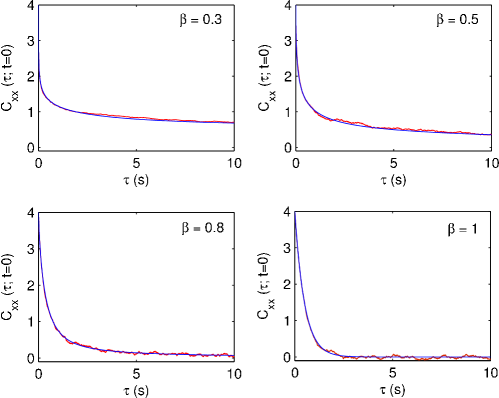
Figure 2: (Color online) Monte Carlo estimates of the autocovariance function $C_{XX}(\Delta t;0|\beta)$ (red irregular lines) compared to the exact result in equation (22) (blue smooth lines) for several values of $\beta$ and $a=2$. Time is in arbitrary units called seconds. The autocovariance functions are not normalized.

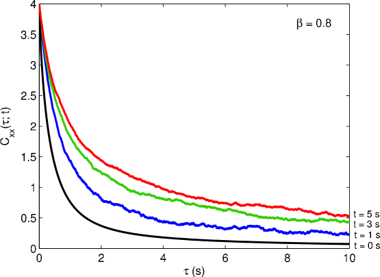
Figure 3: (Color online) Non-normalized autocovariance functions $C_{XX}(\Delta t;t|\beta)$ for $\beta=0.8$, $a=2$ and several values of $t$. Time is measured in arbitrary units called seconds.

IV Discussion and conclusions

The main result of this paper is given in equation (16) for the autocovariance function of a generalized RTS, the double Laplace transform of the probability distribution $P(n,\Delta t;t)$ is given in (19); these results are further specialized to a RTS of Mittag-Leffler type in equation (22). The derivation of such equations is based on renewal theory. The analytical result in equation (16) is then successfully compared to Monte Carlo simulations.

An important feature of a RTS of Mittag-Leffler type is that the renewal density $h(t)$ of the Mittag-Leffler renewal process vanishes for $t\to\infty$ for $0<\beta<1$. Therefore, the hypoteses of the renewal theorem are not satisfied and the stationary regime is never reached. Therefore, contrary to other renewal processes, such as the Weibull process, that, after a transient, become stationary, the renewal process of Mittag-Leffler type is non-stationary also if it is observed far from its beginning. In particular, standard spectral methods fail to describe the features of the RTS of Mittag-Leffler type.

These considerations may be useful when studying the origin of 1/$f$ noise, a problem not addressed here but which will be the subject of a future paper. Indeed, the renewal process of Mittag-Leffler type can be described as an infinite mixture of exponential distributions, for instance, one has for the survival function

$$E_{\beta}\left(-t^{\beta}\right)=\int_{0}^{\infty}g(\mu)\exp(-\mu t)d\mu,$$ (26)

where

$$g(\mu)=\frac{1}{\pi}\frac{\sin(\beta\pi)}{\mu^{1+\beta}+2\cos(\beta\mu)\mu+\mu^{1-\beta}}.$$ (27)

Therefore, based on the ideas developed in mcwhorter55 ; stepanescu74 ; milotti , one already expects to have a power spectrum following a power law. Using the fact that

$$\hat{S}_{XX}(\omega;0|\beta)={\cal F}[C_{XX}(\Delta t;0|\beta)]=\int_{-\infty}^{+\infty}E_{\beta}\left(-2|v|^{\beta}\right)\exp(i\omega v)dv,$$ (28)

one gets

$$\hat{S}_{XX}(\omega;0|\beta)=2\mathrm{Re}[\tilde{C}_{XX}(s=-i\omega;0|\beta)],$$ (29)

and the power spectrum for $t=0$ can be evaluated from equation (21). It turns out that

$$\hat{S}_{XX}(\omega;0|\beta)=2a^{2}\mathrm{Re}\left[\frac{(-i\omega)^{\beta-1}}{2+(-i\omega)^{\beta}}\right]=a^{2}\frac{4\omega^{\beta-1}\sin(\beta\pi/2)}{4+4\omega^{\beta}\cos(\beta\pi/2)+\omega^{2\beta}}$$ (30)

Once again, it must be stressed that, due to non-stationarity, the power spectrum depends on $t$ and not only on the lag $\Delta t$.

- (1) A.N. Kolmogorov, Foundations of the Theory of Probability, (Chelsea, New York, 1956). Translation from German of A.N. Kolmogorov, Grundbegriffe der Warscheinlichkeitrechnung, (Berlin, 1933).
- (2) Kolmogorov’s theorem is the basis for existence (and uniqueness) theorems of stochastic processes. It is discussed in sections 3 and 4 of reference kolmogorov33 .
- (3) S.O. Rice, Bell System Tech. J. 23, 282, (1944). S.O. Rice, Bell System Tech. J. 24, 46, (1945).
- (4) G.W. Kenrick, Phyl. Mag. Ser. 7 7, 176, (1929).
- (5) A. Ya. Khintchin, Math. Annalen 109, 604, (1934).
- (6) H. Cramér, Ann. of Math. Ser. 2 41, 215, (1940).
- (7) A. Mc Whorter, M.I.T. Lincoln Laboratory Report, No. 80, (1955).
- (8) A. Stepanescu, Il Nuovo Cimento 23, 356, (1974).
- (9) E. Milotti, Phys. Rev. E 51, 3087, (1995).
- (10) P. Allegrini, P. Grigolini, L. Palatella, and B.J. West, Phys. Rev. E 70, 046118, (2004).
- (11) W. Feller, An Introduction to Probability Theory and its Applications, vol. 2, (Wiley, New York, 1971).
- (12) D. Cox, Renewal Theory, (Methuen, London, 1967). (first ed. in 1962). D. Cox, V. Isham, Point Processes, (Chapman & Hall, London, 1979).
- (13) C. Godrèche and J.M. Luck, J. Stat. Phys., 104, 489, (2001).
- (14) P.G. Hoel, S.C. Port, and C.J. Stone, Introduction to Stochastic Processes, (Houghton Mifflin, Boston, 1972).
- (15) E. Scalas, Physica A, 362, 225, (2006).
- (16) E. Scalas, R. Gorenflo, F Mainardi, Phys. Rev. E, 69, 011107, (2004). F. Mainardi, R. Gorenflo and E. Scalas, Vietnam Journal of Mathematics, 32 SI, 53, (2004). F. Mainardi, R. Gorenflo, A. Vivoli, Fractional Calculus and Applied Analysis, 8, 7, (2005).
- (17) I.M Gel’fand and G.E. Shilov, Generalized Functions (Academic Press, New York, 1964). Translated from 1958 Russian edition.
- (18) I. Podlubny, Fractional Differential Equations (Academic Press, San Diego, 1999).
- (19) D. Fulger, E. Scalas, and G. Germano, Phys. Rev. E, 77, 021122, (2008).
- (20) A.G. Pakes, Stat. Probab. Lett. 37, 213 (1998).
- (21) T.J. Kozubowski, Stat. Probab. Lett. 38, 157 (1998).
- (22) S. Kotz, T. J. Kozubowski, and K. Podgorski, The Laplace Distribution and Generalizations: A Revisit with Applications to Communications, Economics, Engineering, and Finance, (Birkhäuser, Boston, 2001).
- (23) T.J. Kozubowski and S.T. Rachev, Int. J. Comput. Numer. Anal. Appl. 1, 177 (1999).