Basin boundary, edge of chaos, and edge state
in a two-dimensional model

Abstract

In shear flows like pipe flow and plane Couette flow there is an extended range of parameters where linearly stable laminar flow coexists with a transient turbulent dynamics. When increasing the amplitude of a perturbation on top of the laminar flow, one notes a a qualitative change in its lifetime, from smoothly varying and short one on the laminar side to sensitively dependent on initial conditions and long on the turbulent side. The point of transition defines a point on the edge of chaos. Since it is defined via the lifetimes, the edge of chaos can also be used in situations when the turbulence is not persistent. It then generalises the concept of basin boundaries, which separate two coexisting attractors, to cases where the dynamics on one side shows transient chaos and almost all trajectories eventually end up on the other side. In this paper we analyse a two-dimensional map which captures many of the features identified in laboratory experiments and direct numerical simulations of hydrodynamic flows. The analysis of the map shows that different dynamical situations in the edge of chaos can be combined with different dynamical situations in the turbulent region. Consequently, the model can be used to develop and test further characterisations that are also applicable to realistic flows.

1 Introduction

The transition to turbulence in systems like plane Couette flow or pipe flow differs from the better understood examples of Taylor-Couette or Rayleigh-Benard flow in that turbulent dynamics is observed while the laminar flow is still linearly stable [grossmann00, Ker05, Eck07b, Eckh08]. Evidently, the two types of dynamics coexist for the same parameter values. This suggests a subcritical transition scenario, where the turbulent state forms around the node in a saddle-node bifurcation. Indeed, various bifurcations of saddle-node type have been found in these systems [Nag90, Nag97, Cle97, Wal03, WangGibsonWaleffe2007, Eck02, Fai03, TW_bristol, Pri07, aberdeen] but at least in pipe flow they differ from the standard phenomenology in that the node state is not stable but has unstable directions as well: it is like a saddle-node bifurcation in an unstable subspace. Numerical studies of pipe flow [Sch07a]and some simplified models [Sku06] show that also the ‘saddle state’ has peculiar features. In the higher-dimensional space it need not be a fixed point, as in the traditional saddle-node bifurcation scenario, but can be dynamically more complicated, i.e., periodic or even chaotic.

In Couette and pipe flow the turbulent state forming around the node need not be an attractor. Indeed, numerical and experimental evidence indicates that at least in the transitional regime the turbulent dynamics is not persistent but transient [brosa91, bead_bottin1, bead_bottin2, Moe04, FE04, Hof06, Mul05, Mul06, Pei06, Pei07, Schn08b]. Nevertheless, it is still possible to define a boundary between trajectories directly decaying into the laminar state and those first visiting the neighbourhood of the chaotic saddle. Trajectories on the turbulent side show a sensitive dependence on initial conditions and give rise to rapidly varying lifetimes. This suggested the name “edge of chaos” for this boundary [Sku06]. In the case of the standard subcritical transition scenario, this edge of chaos is given by the saddle state and its stable manifold [Ott2002]. There is some evidence that for such a behaviour in plane Couette flow [WangGibsonWaleffe2007, SchneiderGibson2007]. In the case of pipe flow numerical evidence suggests that the saddle state is not a single fixed point or a travelling wave, but that it rather carries a chaotic dynamics [Sch07a].

In order to explore some of the possibilities in a computationally efficient and dynamically transparent manner, we turn to a specifically designed model system. In the following we will describe a two-dimensional map that shows much of the phenomenology observed in transitional pipe flow, and at the same time has parameters that allow us to discuss the transitions and crossover between different kinds of dynamical behaviour. We use the model to study the boundary between laminar and turbulent dynamics, and the dynamics in this boundary. In particular, we will argue that the edge of chaos and the edge states introduced in Sku06 and Sch07a are the natural extension of the basin boundary concept to situations where the turbulent dynamics is transient.

Studying boundaries of basins of attraction has a long history in dynamical systems. It goes back to Cayley for the case of Newton iteration, and to Julia and Fatou for dynamical systems defined in the plane of complex numbers [peitgen, Devaney2003]. To make contact with differential equations much follow up work focussed on the conceptually simplest systems of flows in three dimensions, or equivalently 2d invertible maps. In principle the generic properties of the boundaries between the domains of attraction of different types of invariant sets (sinks, saddles nodes, limit cycles, and chaotic sets) have exhaustively been classified [RobertAlligoodOttYorke2000, Ott2002] for these systems by considering (i) the possible sections of the respective stable and unstable manifolds and (ii) the possible impact of (dis-)appearance of stable orbits in saddle-node bifurcations. However, careful inspections of the parameter dependence of ‘explosions’, where the features of invariant sets alter qualitatively, can occasionally still unearth surprises in systems as simple as the Henón map [Osinga2006]. Higher-dimensional chaos (“hyperchaos”) shares common themes with low-dimensional chaos [Roessler1983], but there also are important differences due to the additional freedom of changing dynamical connections between chaotic sets [GrebogiOttYorke1983PRL, LaiWinslow1995, DellnitzFieldGolubitskyHohmannMa1995, AshwinBuescuStewart1996, KapitaniakMaistrenkoGrebogi2003, RempelChianMacauRosa2004a, PazoMatias2005, TelLai2008]. Besides fluid mechanics other important fields of applications of hyperchaos are transition state theory [KovacsWiesenfeld2001, WigginsWiesenfeldJaffeUzer2001, WaalkensBurbanksWiggins2004, BenetBrochMerloSeligman2005] and the quest for the (domain of) stability of irregular and stable synchronised states in systems of coupled oscillators (see PikovskyRosenblumKurths2001 PikovskyRosenblumKurths2001 for an overview). Considerable insight in the latter problem come from studies of two symmetrically coupled logistic maps [YamadaFujisaka1983, FujisakaYamada1983, GuTungYuanFengNarducci1984, PikovskyGrassberger1991, MaistrenkoMaistrenkoPopovichMosekilde1998, KapitaniakLaiGrebogi1999, KapitaniakMaistrenkoGrebogi2003]. More recently also the generalisations to asymmetric coupling [HuYang2002, KimLimOttHunt2003] and more complex maps [Lai2001, KimLimOttHunt2003, AshwinRucklidgeSturman2004] have been explored.

The present study is motivated by observations on the turbulence transition in situations where the laminar profile is linearly stable, and hence will use descriptions like ‘laminar’ and ‘turbulent’ to describe the two dominant state between which we would like to determine the basin boundary or edge of chaos. One of our principle interests will be in situations where the dynamics on the edge of chaos separating (transient) turbulence and laminar motion is chaotic. To that end our model must have at least two continuous degrees of freedom — one degree of freedom for the dynamics in the edge, and a second one perpendicular to it. A minimal model of the phase-space flow would then require at least a four-dimensional invertible map, but then we would loose the advantages of the graphical representation of the invariant sets and their domains of attraction that are available in lower dimensions. As in the approaches to model synchronisation of coupled nonlinear oscillators, we will therefore design a system of two coupled 1-d maps.

The paper has three main parts. In the first part (section 2) we introduce the model, discuss the dynamics of the uncoupled case, and introduce the considered coupling. The second part (sections 3 and 4) deals with the dynamics of two coexisting attractors: In section 3 we discuss the shape and dynamics of the attractors, and the transient dynamics in the respective basins of attraction. Section 4 addresses the dynamics of the relative attractor on the basin boundary between the attractors, and how this dynamics effects the shape of the separating boundary. In the third part of the paper we turn to the case of a chaotic repellor in the turbulent dynamics which mimics turbulent transients decaying to a laminar flow profile: Section 5 deals with the case of a chaotic saddle coexisting with a fixed point attractor. We discuss the metamorphosis of the basin boundary at the crisis where the attractor turns into a chaotic saddle. Finally, in section 6 we conclude the paper with summarising remarks and discuss how the findings on this 2D model relate to observations in shear flows such as turbulent pipe and plane Couette flow.

2 The two-dimensional map

To admit coexistence of laminar and a turbulent dynamics one degree of freedom of the map must be chosen along a phase-space direction separating regions with these different types of dynamics. A second degree of freedom is needed to capture the dynamics perpendicular to this direction, and to allow for dynamics within the boundary between laminar and turbulent dynamics. We think of the two coordinates of the map as representing the energy content of the perturbation ($x$-direction) and the dynamics in an energy shell ($y$-coordinate). The $x$-coordinate interpolates between a laminar and a turbulent dynamics. The $y$-coordinate models all other degrees of freedom. In the latter direction the map is globally attracting towards a region near $y=1$. The combined map has a fixed point, corresponding to the laminar profile, and — for suitable parameter values — also a region with a chaotic dynamics corresponding to turbulent behaviour. In the following we first describe the two uncoupled maps in $x$ and $y$, and then we discuss their coupling and its consequences for the dynamics.

2.1 Dynamics in $x$

For the dynamics along the energy axis, we use a map that has a stable fixed point at $x=-2$, and a chaotic dynamics for $x>0$. The former corresponds to laminar flow, and the latter mimics turbulent motion. An intermediate fixed point at $x=0$ separates the laminar region $x<0$ from the turbulent one at $x>0$. It is unstable. These features are contained in the one-parameter map [figure 1(a)]

$$x_{n+1}=f(x_{n};a)$$ (1a)

with

$$f(x;a)=\left\{\begin{array}[]{ll}a\,x\,(1-x)&\textrm{for}\quad x>x_{*}\equiv\left.\left(1-\sqrt{1+8/a}\right)\right/2\\ -2&\textrm{else}\end{array}\right.$$ (1b)

Here $x_{*}$ is the leftmost intersection between the constant value $-2$ for $x<x_{*}$, and the quadratic part at $x>x_{*}$. With this choice the map is continuous.

   

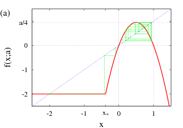
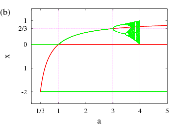
Figure 1: The map along the $x$-direction. (a) The red line shows the function $f(x;a)$ for $a=3.8$, and the green ones indicate the evolution of two trajectories starting at $x=\pm 0.1$, respectively. The maximum of the map is always at $x=1/2$, irrespective of the value of $a$, and takes the value $f(x=1/2;a)=a/4$. The initial condition $0.1$ approaches the chaotic attractor in $[f(1/2);f^{2}(1/2)]=[0.18;0.95]$, and the one starting at $-0.1$ approaches the fixed point at $x=-2$. (b) Bifurcation diagram of the map $f(x;a)$. Green dots represent points on either of the two attractors of the map, and the red lines unstable fixed points.

The bifurcation diagram for this map is shown in figure 1(b). We will only be interested in parameter values $a>1/3$ where $x_{*}>-2$. In this case the map has a stable fixed point at $x=-2$, which absorbs all initial conditions starting outside the interval $[0,1]$. Over the interval $x\in[0,1]$ the map coincides with the logistic map and shows its familiar bifurcation diagram. For all $1/3<a<1$ there are stable fixed points at $x=-2$ and $x=0$. In addition, there is an unstable fixed point at $x_{s}=1-1/a$, which lies between $-2$ and $0$. At $a=1$ the fixed point $x_{s}$ crosses $x=0$, and the two fixed points change stability in a transcritical bifurcation. For $a>1$ the point $x=0$ is unstable, and $x_{s}$ is a stable fixed point. At $a=3$ the fixed point $x_{s}$ undergoes a first period doubling, and subsequently follows the period-doubling route to chaos. Beyond $a\simeq 3.59$ there are chaotic bands extending from $f(1/2;a)=a/4$ down towards $f^{2}(1/2;a)=f(a/4;a)=(a/2)^{2}\,(4-a)$.

At $a=4$ the chaotic band generated by the period doubling collides with the unstable fixed point at $x=0$, leading to a boundary crisis [greb82, GrebogiOttYorke1983, GrebogiOttRomeirasYorke1987, Ott2002]. For $a>4$ some points near the maximum of the parabola are mapped outside the interval $[0,1]$ and the attractor turns into a chaotic saddle. All points except for a Cantor set of measure zero will eventually map outside the interval and then be attracted to the laminar fixed point at $x=-2$. The Cantor set contains an infinity of orbits which follow a chaotic dynamics and never leave the interval tel1990,Ott2002cf. .

In summary, depending on the parameter values, the $x$-map shows the coexistence of a stable laminar state with one of three possible types of non-laminar dynamics: another fixed point, a chaotic attractor, or a chaotic saddle. The coexistence of a stable laminar fixed point at $x=-2$ with a transient chaotic dynamics in the map for $a>4$ mimics the coexistence of a transient turbulent dynamics with a linearly stable laminar steady flow. The direct domain of attraction of the laminar state at $x=-2$ is bounded towards positive $x$ by an unstable fixed point at $x=0$.

2.2 Dynamics in $y$

The $y$-dynamics represents the motion within the energy shell. In the simplest case it is globally attracting towards a globally stable fixed point. Then only the $x$-dynamics matters, and it represents the dynamics along its unstable direction. In order to model the motion in the energy shell we consider a unimodal (i.e., a single-humped) map of Lorentzian type (figure 2(a)) that maps large $|y|$ towards the region $y\simeq 1$,

$$y_{n+1}=g(y_{n};b)\,,$$ (1ba)

with

$$g(y;b)=\frac{2}{1+b\,(y-1)^{2}}\,.$$ (1bb)

   

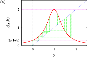
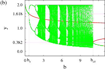
Figure 2: The map in the $y$-direction. (a) The function $g(y;b)$ for $b=6$, and the trajectory of $y=0$. For all $b$ the maximum of $g(y;b)$ is at $\left(y,g(1;b)\right)=(1;2)$. Moreover, $g(2;b)=g(0;b)=2/(1+b)$ such that the attractor of the map always lies in the interval $[2/(1+b);2]$. (b) Bifurcation diagram of the map $g(y;b)$. As in Fig. 1 green dots represent points on the attractor, and the red lines mark two unstable fixed points of particular interest.

In its first iteration the map collects all initial conditions into the interval $[0,2]$. In this interval the map can have up to three fixed points $y_{p}$. For the discussion of the properties of the map and the fixed points, it is convenient to solve the fixed point equation for the parameter and to study

$$b_{0}(y_{p})=\frac{2-y_{p}}{y_{p}\,(y_{p}-1)^{2}}\,.$$ (1bc)

By evaluating $\textrm{d}b_{0}/\textrm{d}y_{p}=0$ one verifies that there is a saddle-node bifurcation at the critical value $y_{cr}=\left(3-\sqrt{5}\right)/2\simeq 0.382$. This corresponds to the parameter value $b_{cr}\equiv b_{0}(y_{cr})\simeq 11.09$. Consequently, there is only a single fixed point for $b<b_{cr}$, and there are three fixed points for larger values of $b$.

Making use of equation (1bc) in order to evaluate $\textrm{d}g(y;b)/\textrm{d}y=-1$ one verifies that the single fixed point is stable for $y>y_{s}=\left(1+\sqrt{5}\right)/2\simeq 1.6182$, i.e., for $b<b_{s}\equiv b_{0}(y_{s})\simeq 0.618$. Beyond $b_{s}$ the fixed point undergoes a period-doubling route into chaos, and produces a broad chaotic band in the interval $[0,2]$. At $b_{cr}$ there is a saddle-node bifurcation in the support of the attractor, which transforms the attractor into a saddle. For larger values of $b$ this saddle coexists with a globally stable fixed point.

For later reference we introduce also the Lyapunov number $\Lambda$ of the map, which describes how a small distance $\delta y_{0}=|y^{(a)}_{0}-y^{(b)}_{0}|$ between two close-by initial conditions $y^{(a)}_{0}$ and $y^{(b)}_{0}$ grows with the number $j$ of iterations,

$$\delta y_{j}\equiv|y^{(a)}_{j}-y^{(b)}_{j}|\sim\delta y_{0}\;\Lambda^{j}\,.$$ (1bd)

The Lyapunov numbers can be defined for invariant sets, such as the maximal chaotic invariant set ($\Lambda_{c}$) and for the attractor ($\Lambda_{a}$). The distinction is important whenever the two numbers do not coincide, as in cases where an attracting periodic orbit is surrounded by an invariant chaotic set. The two Lyapunov numbers for the map (1bb) are shown in figure 3. The Lyapunov number for the maximal chaotic invariant set is shown as a solid red line: it always remains above $1$. The Lyapunov number of the attractor is shown by a dotted green line. It takes values smaller than unity in the parameter windows where there is an attracting periodic orbit.

In summary, the main features of the $y$-dynamics are that it is globally contracting towards the interval $[0;2]$, and that depending on the parameter values one can have one of three types of invariant sets: (i) a stable periodic orbit of period $2^{n}$ with $n=0$ (i.e., a fixed point) for $b<b_{s}$ and larger $n$ in the subsequent period doubling cascade; (ii) a chaotic attractor for numerous parameters in the range $b_{s}<b<b_{cr}$; or (iii) a chaotic saddle coexisting with a periodic orbit (in the periodic windows of the previous parameter regime) or a fixed point for $b_{cr}<b$.

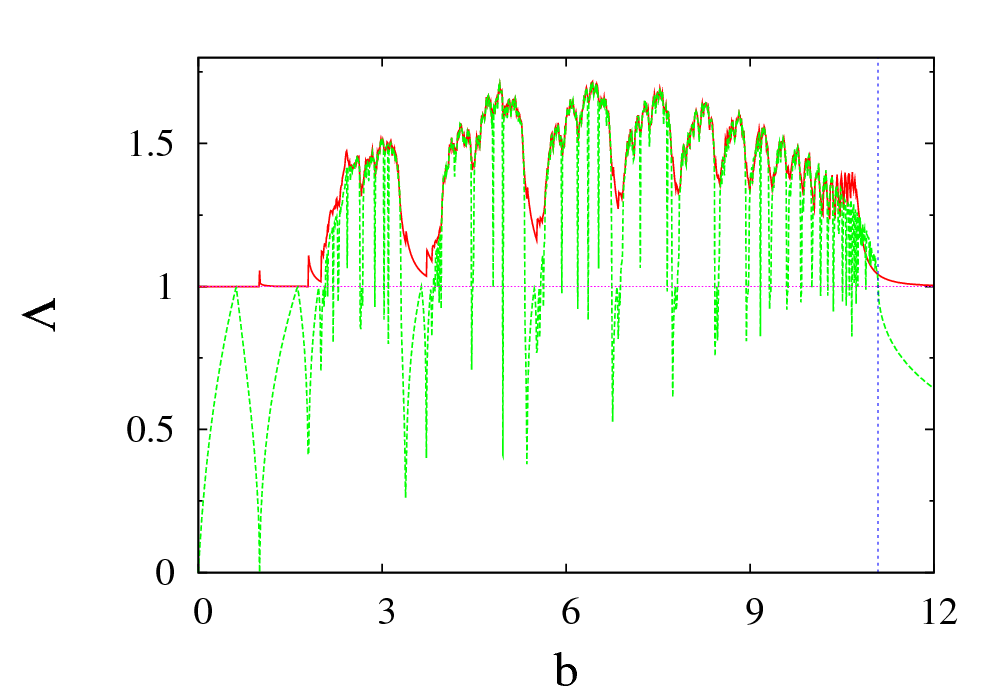
(a)   (b)  

Figure 3: Lyapunov number $\Lambda$ of the attracting set (green) and the chaotic invariant set (red) of the map (1bb). The former number is obtained from the last $2\cdot 10^{6}$ iterates of a trajectories that is $10^{7}$ iterations long, and the latter by means of the thermodynamic formalism [cf. tel1988 tel1988,tel1990 for a description of the algorithm]. (b) Magnification of a small parameter interval to show that in regions where, within numerical uncertainty, there are no stable periodic orbits, the two Lyapunov numbers coincide.

2.3 The coupling

Without a coupling between the two maps, the three possibilities in the $x$-dynamics combine with the three possibilities in the $y$-dynamics for nine different regimes. Now we introduce a coupling between both degrees of freedom. The specific form of the coupling should not be important if it preserves a few properties. For instance, we want to keep a locally stable fixed point for the laminar state also in the coupled dynamics. Specifically, the $y$-map should have a stable fixed point at $x=-2$. We therefore introduce an $x$-dependence in the parameter $b$ of the $y$-map such that the coupling vanishes for $x\simeq-2$, thereby maintaining the stability properties of the uncoupled map:

$$b(x)=\gamma\,(2+x)\,.$$ (1be)

We refer to this fixed point as the laminar fixed point. Since the non-trivial $x$-dynamics lies within the interval $[0,1]$, the range of $b$ values varies between $2\gamma$ and $3\gamma$, so that the parameter $\gamma$ selects the type of $y-$dynamics for the chaotic regime in the $x$ dynamics.

To complete the coupling we also introduce an influence of the $y$-dynamics on the $x$-dynamics, since otherwise the bifurcations are determined by the $x$-map alone: we shift $x_{n}$ by the deviation of $y_{n}$ from the position of the maximum before applying the mapping, i.e.,

$$x_{n+1} = f(x_{n}-\epsilon\,(y_{n}-1);a)$$ (1bfa)

$$y_{n+1} = g(y_{n};b(x_{n}))$$ (1bfb)

with the specific forms (1b), (1bb), and (LABEL:parYx) for $f(x)$, $g(x)$, and $b(x)$, respectively. In this paper we will concentrate on the weak-coupling limit where $\epsilon\ll 1$. Unless stated otherwise this parameter will always take the value $\epsilon=0.03$.

This completes our definition of the coupled map. Through appropriate choices of the parameters $a$ and $\gamma$ we can — one by one — study the nine parameter regimes with their qualitatively different dynamics. We here begin with the six cases where the non-laminar $x$-dynamics is attracting, and a laminar and a non-laminar attractor coexist. The case of a transient dynamics will be taken up in section 5.

3 Two coexisting attractors

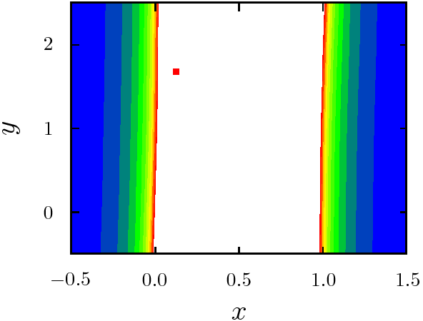
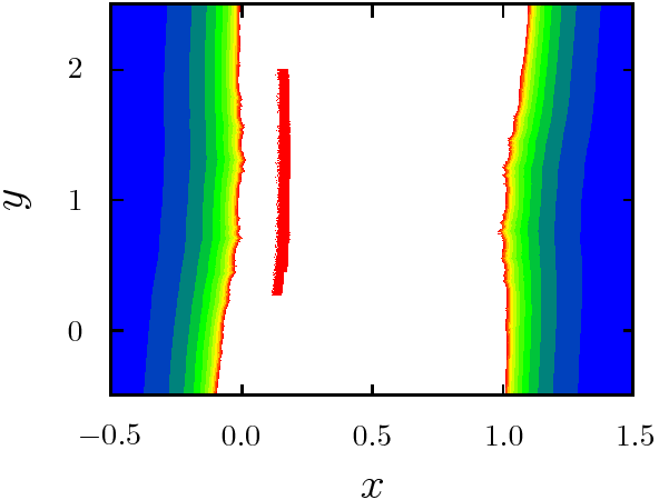
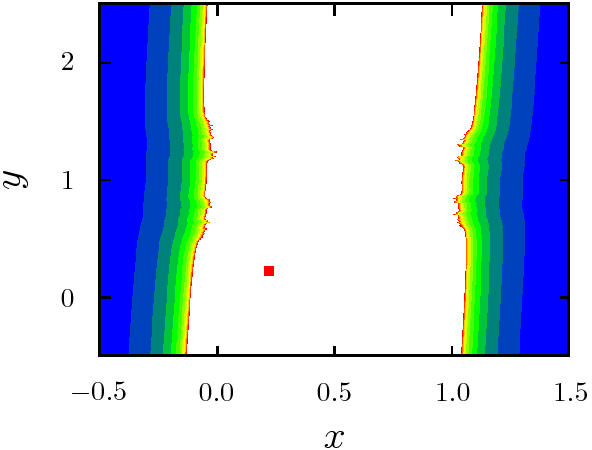
  (a)   (d)
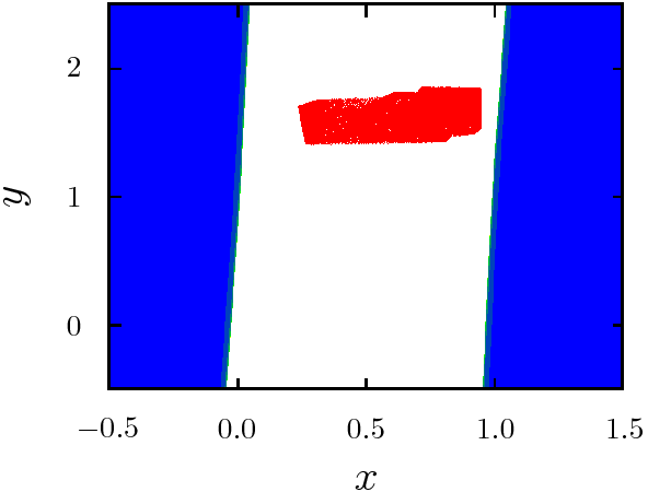
  (b)   (e)
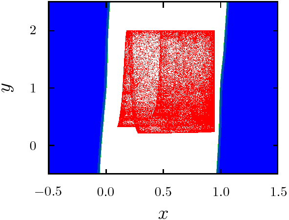
  (c)   (f)

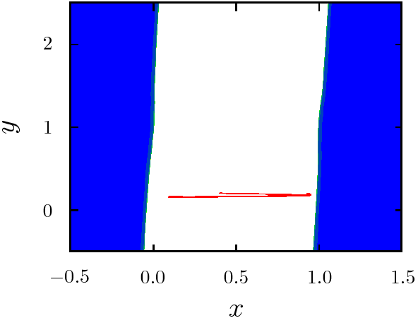
Figure 4: For initial conditions $(x,y)$ the colours indicate the number of iterations required to reach the laminar fixed point. The colour code runs from one iteration (blue) to more than ten iterations (red). Initial conditions in the white region are attracted to the chaotic attractor, which is also shown by red dots. The panels in different rows refer to different values of $\gamma$: (a,d) $\gamma=0.2$, (b,e) $\gamma=3$, and (c,f) $\gamma=6$, respectively. In these cases the $y$-dynamics shows a single fixed point, chaos, and a fixed point coexisting with a chaotic saddle, respectively. The left panels (a–c) and right panels (d–f) refer to $a=1.2$ and $a=3.8$, respectively. For the panels (a–c) the non-laminar $x$-dynamics amounts to a fixed point, and for (d–f) it is chaotic. In all panels $\epsilon$ is set to $0.03$, except for the top left one, where $\epsilon=0.01$, because in the latter case the non-trivial fixed point at $x>0$ disappears for $\epsilon\gtrsim 0.012$.

3.1 Attractors and basins

Figure 4 shows the domain of attraction of the laminar fixed point together with the non-laminar attractor. The panels on the left-hand side refer to $a=1.2$ immediately beyond the crossing of stability, where $f(x,a)$ has a stable fixed-point attractor at $x=1-1/1.2\simeq 0.17$. The panels on the right-hand side refer to $a=3.8$. In this case the fixed point at $x=-2$ coexists with a chaotic attractor. Without coupling, for (1bfa) with $\epsilon=0$ the attractor is located in the interval $[0.18;0.95]$.

For $\gamma=0.2$ [figure 4(a,d)] the iteration of $y$ directly approaches the fixed point at $y\simeq 1.8$, and subsequently only wiggles around this point due to the perturbation arising from the $x$-dynamics.

For $\gamma=6$ [figure 4(c,f)] the iteration of $y$ approaches the fixed point at $y\simeq 0.38$. However, in this case the fixed point is surrounded by a chaotic saddle, and the approach may involve long chaotic transients.

Finally, for $\gamma=3$ [figures 4(b,e)] the parameter $b(x)$ varies between $6$ and $9$ for $x$-values in the interval $[0,1]$. For parameter values $a$ slightly below $4$ one hence obtains a chaotic dynamics for both $x$ and $y$. In this case the attractor varies over a considerable range of $y$-coordinates, and one can clearly see the strong influence of the coupling. When there are broad chaotic bands in both directions [figure 4(e)] the attractor can even extend to negative values of $x$.

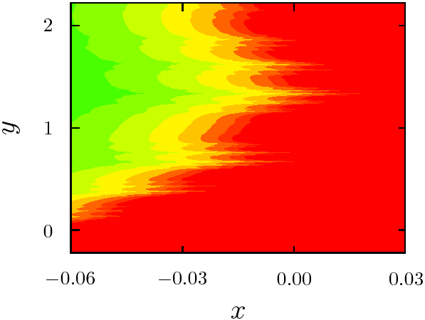
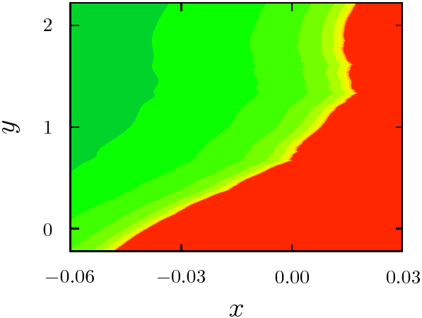
  (a)   (b)
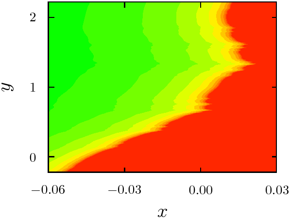
  (c)   (d)

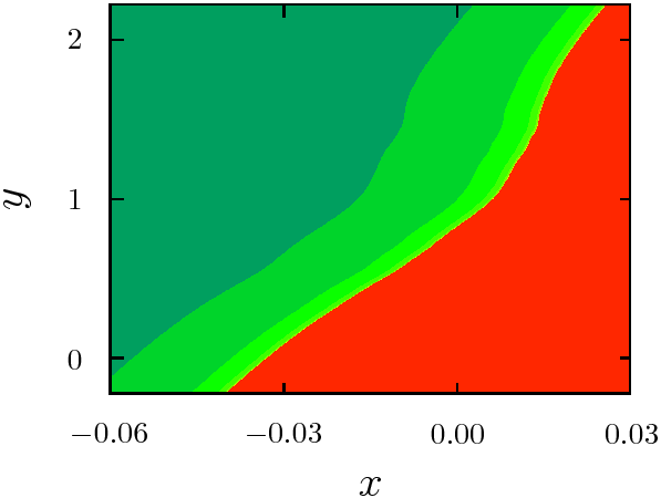
Figure 5: Magnifications of the boundary between the region of initial conditions approaching the laminar fixed point at $(-2,2)$, and the chaotic attractor at $x>0$ for $\gamma=3$, $\epsilon=0.03$, and different values of $a$: (a) $a=1.2$, (b) $a=1.6$, (c) $a=2.0$, (d) $a=3.8$. All initial conditions which approach the attractor to the right are shaded in red, and the colour gradient from blue to yellow indicates the number of steps it takes to reach the laminar fixed point with the colour coding also used in figure 4. The cross-over from a rough to a smooth boundary arises at $a\simeq 1.6$.

3.2 The boundary between the two attractors

We now focus on the boundary separating the basins of attraction of the laminar and the chaotic attractor to the left and right, respectively. If $\epsilon=\gamma=0$, it coincides with the $y$-axis: All initial conditions with $x>0$ are attracted to the turbulent dynamics, and the ones with $x<0$ to the laminar state. Moreover, all points with $x=0$ are immediately mapped into the hyperbolic fixed point $(0,2)$. The hyperbolic fixed point then becomes a relative attractor, since it is an attractor for initial conditions in the boundary between the two attractors. For $\epsilon$ and $\gamma$ nonzero but small, the hyperbolic point is slightly shifted, and the boundary no longer coincides with the $y$-axis, but it remains smooth. The boundary can be determined by picking initial conditions with, say, prescribed $y$ and varying $x$ and following them for some iterations forward in time: it can then be bracketed by a pair of $x$-values where one initial condition iterates towards the laminar state and the other towards the turbulent one. This method allows us to track the dynamics in the boundary not only in the case where the relative attractor is a fixed point, but also when it is more complicated. In a hydrodynamic setting this approach has been explored in the framework of low-dimensional shear flow models [Sku06] and direct numerical simulation of pipe flow [Sch07a].

In figure 4 the boundary between the two attractors is the boundary of the region shaded from blue to yellow. It appears to be smooth for $a=3.8$ and for $\gamma=0.2$. In contrast, it looks irregular for $a=1.2$ and $\gamma=3$ or $6$ [figures 4(b,c)]. The magnifications in figure 5 confirm the roughness of the boundary and indicate a crossover from a smooth to an irregular boundary as $a$ decreases from $3.8$ to $1.2$, with $\gamma=3$ and $\epsilon=0.03$ fixed.

There are two elements needed to understand the emerging roughness of the boundary: the first one is the observation that states in the boundary are attracted to a subset of the boundary itself, i.e., the dynamics in the basin boundary converges to an edge state. The second observation is that when the edge state is chaotic a rough boundary can form provided that the Lyapunov exponent for the chaotic motion on the basin boundary is larger than the one characterising the escape from the boundary. These two aspects are discussed in the next section.

4 Edge states and relative attractors

4.1 Identifying the edge state

In order to follow a trajectory for long times and to be able to identify the relative attractor, the bracketing of trajectories in the boundary described in section 3.2 has to be refined after some time. After all, the distance between the trajectories in the pair bracketing the trajectory on the boundary grows exponentially with the number of iterations. Specifically, we proceed as follows. We take initial conditions for the two trajectories that have equal $y$-values and $x$-values separated by less than $10^{-6}$. The two trajectories are followed until $\max(\delta x_{j},\delta y_{j})$ exceeds $5\cdot 10^{-3}$. Then a new pair is determined with $y_{0}=(y^{a}_{j}+y^{b}_{j})/2$ and $\delta x_{0}<10^{-6}$. An alternative approach could start from the observation that the line connecting the two trajectories will be oriented along the direction of the largest Lyapunov exponent of the map and search for a refinement along this line. Here and in the previous applications to pipe flow [Sch07a, SchneiderEckhardt2008] it was observed that the first approach, which repeatedly projects the line segment between the two points to a fixed direction in space, is more robust and converges more reliably, especially in cases where the geometry of the boundary is complex.

The dynamics in the edge state is explored further in figure 6. Presented are two situations where the boundary shown in figure 5 appears smooth ($a=1.2$, left column) and rough ($a=3.8$, right column), respectively. The two frames in figure 6(a) show trajectories on the boundary constructed by the edge tracking algorithm. The trajectories nicely reproduce the features of the boundaries also shown in figure 5(a) and (d). The difference between the two figures is that the boundary in figure 5 emerges from a two-dimensional search, whereas the one in 6 is determined by a following a single trajectory. This allows us to show the time series of the coordinates of edge trajectories and the associated return maps for the $y$-coordinates in row (b) and (c), respectively. By visual inspection it is very hard to see differences to the unperturbed dynamics of $g(y;b(0))$.

To demonstrate effects introduced by the coupling of the dynamics to the unstable $x$-direction we subtract the functional form of the $y$-map. The deviations from the unperturbed $y$-dynamics, $\delta y_{n}=y_{n+1}-g(y_{n})$, differ substantially for smooth and rough boundaries: For $a=3.8$ the iterates lie on a smooth, double valued curve. Its double-valuedness reflects the influence of a non-trivial dynamics in $x$, which follows iterates of a map with a single bump, see the iterates in row (e). However, the relation between $x$ and $y$ is single valued, and therefore there is not much disorder. For $a=1.2$, the distribution of iterates looks rather noisy (e), and no simple relation between their images can be found.

Note that in both cases the dynamics in $y$ is chaotic, and along the $x$-direction close-by trajectories escape exponentially from the vicinity of the boundary: both Lyapunov numbers are positive. On the other hand, for $a=3.8$, the different branches of the return map come to lie on a smooth invariant set, while for smaller $a$ the basin boundary is a rough invariant set. In the next subsection we argue that this difference is due to a crossover of the absolute values of the Lyapunov numbers, just as it has been discussed in the context of unstable-unstable pair bifurcations [GrebogiOttYorke1983PRL, TelLai2008].

  (a)  
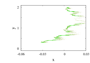
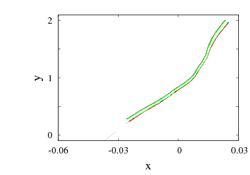
  (b)  
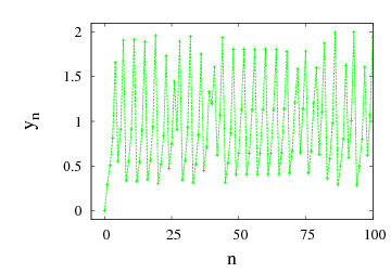
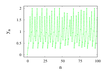
  (c)  
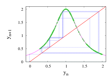
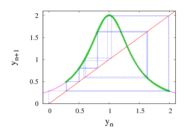
  (d)  
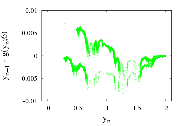
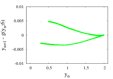
  (e)  

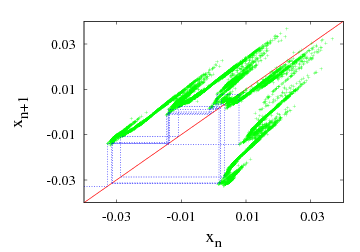
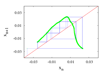
Figure 6: Evolution of trajectories on the boundary separating convergence to laminar and to turbulent motion ($\gamma=3$ and $\epsilon=0.03$ for all panels; left panels: $a=1.2$; right panels: $a=3.8$). (a) The trajectories on the boundary trace out the shape of the boundary, which is rough for $a=1.2$ and smooth for $a=3.8$. For later reference the right panel also shows the edge of chaos for $a=4.2$ beyond the crisis of the attractor. It has been shifted by $(x;y)=(0.001;-0.04)$ to the lower right. (b) When started at $x=0$ the trajectories rapidly converge to a chaotic attractor located in the interval $y\in[2/7;\,2]$. (c) Return map for the $y$-coordinate. Within numerical accuracy it agrees with $g(y;6)$ (solid red line). The first ten iterations are explicitly indicated — the points visited during the initial 10000 time steps are indicated by green crosses ($+$). (d) Deviation of the values plotted in (c) from the function $g(y;6)$. (e) Return map for the $x$ coordinate. The first iterations and subsequent points indicated as in panel (c).

4.2 Transition between smooth and rough boundaries

Close to $a=1.6$ the boundary crosses over from a highly irregular geometry to a line with only few kinks, whose number progressively decreases for even larger values of $a$. Similar transitions between rough and smooth boundaries have previously been seen in unsteady-unsteady pair bifurcations [GrebogiOttYorke1983PRL, Ott2002] and phase-synchronised chaos [Hunt97, Rosa1999]. They are related to a crossover of the two Lyapunov numbers of the map. To gain insight into the transition we estimate the slope $|\delta y_{0}/\delta x_{0}|$ of the boundary at a point $(x_{0},y_{0})$. Linearising equation (1bfa) around the iterates $(x_{j},y_{j})$ of the considered point we find

$$\delta x_{j+1}\equiv f^{\prime}\left(x_{j}-\epsilon(y_{j}-1)\right)\;\left(\delta x_{j}-\epsilon\delta y_{j}\right)=\sigma_{j}\;\left(\delta x_{j}-\epsilon\delta y_{j}\right)$$ (1bfg)

where $\sigma=f^{\prime}(x)=a\,(1-2x)$ is the derivate of $f(x;a)$. Since all points lie on the boundary, $x_{j}-\epsilon\,(y_{j}-1)$ is close to zero for all $j$, as can also be verified by inspection of figures 4 and 5. Consequently, $f^{\prime}$ is always evaluated at a point close to zero, and $\sigma_{j}$ takes values close to $a$. By recursively working out equation (1bfg) we find

$$\delta x_{n}= \left(\prod_{k=1}^{n}\sigma_{n-k}\right)\;\delta x_{0}-\epsilon\;\sum_{j=1}^{n}\;\left(\prod_{k=1}^{j}\sigma_{n-k}\right)\;\delta y_{n-j}$$

$$\Longleftrightarrow\quad \delta x_{0}= \frac{\delta x_{n}}{\prod_{k=1}^{n}\sigma_{n-k}}+\epsilon\;\sum_{j=0}^{n-1}\;\frac{\prod_{k=1}^{j}\sigma_{n-k}}{\prod_{k=1}^{n}\sigma_{n-k}}\;\delta y_{n-j}$$ (1bfh)

For an initial perturbation which is located on the boundary the deviation $\delta x_{n}$ is bounded, and — in the present case — in absolute value it is much smaller that unity. (cf. figure 5). On the other hand, for large $n$ the denominator $\prod_{k=1}^{n}\sigma_{n-k}$ takes on very large values — after all, $a>1$ and $\sigma_{k}\simeq 1$. Consequently,

$$\delta x_{0}\simeq\epsilon\;\sum_{j=0}^{n-j-1}\;\frac{\delta y_{n-j}}{\prod_{k=0}^{j-1}\sigma_{k}}$$ (1bfi)

In the limit of very small perturbations and large $n$ we can approximate the product by its asymptotic scaling, i.e.,

$$\prod_{k=0}^{n-1}\sigma_{k}\sim a^{n}\,.$$

In addition, according to equation (1be) the parameter $b$ of $g$ always takes values very close to $2\gamma$ because all $x_{j}$ are very close to zero. As shown in figure 6(c) the dynamics of the $y$ coordinate essentially amounts to the unperturbed dynamics such that we may use equation (1bd) to related $\delta y_{j}$ to $\delta y_{0}$.

In the scaling regime the sum in equation (1bfi) can be worked out, yielding

$$\left|\frac{\delta x_{0}}{\delta y_{0}}\right|\sim\epsilon\>H\;\frac{H^{n}-1}{H-1}\qquad\hbox{ with }\quad H=\frac{\Lambda}{a}\,.$$ (1bfj)

In the limit $n\rightarrow\infty$ the right hand side of equation (1bfj) remains finite only if $H<1$. Hence, the boundary will be smooth for $H<1$, or $\Lambda<a$. On the other hand the bound (1bfj) diverges for $H>1$. In this case the slope diverges at least for some points on the boundary, which will hence be rough.

As noted above for points on the boundary the parameter $b$ of $g$ always takes values very close to $2\gamma$. According to figure 3 one thus finds that $\Lambda\simeq 1.59$ for $\gamma=3$. The crossover from a rough to a smooth boundary should therefore occur at $a\simeq 1.59$, which is in excellent agreement with the numerical findings of figure 5.

This completes the characterisation of the attractors and their basin boundary. In the following section we address the case of a chaotic saddle coexisting with a laminar fixed point.

5 Transient chaos

5.1 Lifetime Plots

The six cases discussed in the preceding sections cover the cases of coexisting attractors. However, close to the transition in plane Couette flow and pipe flow the turbulent dynamics is transient, so that also the cases of a coexistence between a laminar fixed point and a chaotic saddle that supports transient chaotic dynamics are of interest. Our map realizes this for $\epsilon=0.03$ and $a\gtrsim 4$ (see figure 7). As in figure 4 we consider the three cases (a) $\gamma=0.2$, (b) $\gamma=3$ and (c) $\gamma=6$.

When the parameter $a$ exceeds a critical value $a_{cr}(\gamma)$, the laminar fixed point becomes globally attracting except for a measure zero set containing periodic and aperiodic trapped orbits left over from the attractor. This is apparent in the plots in figure 7, which show the lifetime of initial conditions $(x,y)$ for $a=4.0$ and different values of $\gamma$. For $\gamma=0.2$ [figure 7(a)] the critical value $a_{cr}$ is larger than $4.0$, i.e., there still is a stable chaotic attractor coexisting with the laminar fixed point. However, we already see two ‘fingers’ approaching the attractor from the top and from the bottom. When increasing either $\gamma$ or $a$ these fingers are joined by additional narrower fingers which all simultaneously collide with the attractor at the parameter value $a_{cr}(\gamma)$. Beyond this crisis most of the trajectories of the former attractor escape through the regions where the collision took place [Ott2002]. The orbits of the attractor which never enter the regions form a chaotic saddle.

The panels figure 7(b,c) show the situation beyond the crisis. The blue areas iterate to the laminar fixed point in one and two iterates, respectively. The dark green strips near $x\simeq 0$ and $x\simeq 1$ arrive at the fixed point in three iterations, and initial conditions in the widest fingers (also dark green) pointing towards $(x,y)=(0.5;1)$ escape to the laminar fixed point in four iterations. On the next level there are four lighter green fingers lying between the widest fingers and the outer regions ($0<x<0.5$ and $0.5<x<1$), respectively, which are mapped to the fingers near $x\simeq 0.5$. With each additional iteration, the number of fingers doubles. At the crisis all fingers simultaneously collide with points lying at the upper and lower boundaries of the attractor. They can be interpreted as a primary collision of the attractor with its basin boundary, and the simultaneous collision of all the pre-images of this point.

What happens to the basin boundary of the attractor when going through the crisis? The chaotic attractor embedded in the basin boundary merges with the attractor. We have seen that this generates a fractal set of “holes” (actually the fingers) through which trajectories of the former attractor escape to the laminar fixed point. The chaotic trajectories that never enter the fingers form a Cantor set. Since trajectories starting in the domain of attraction are attracted towards (a small neighbourhood of) the Cantor set and those starting in the vicinity of this set escape almost certainly to the laminar state, the Cantor set forms a chaotic saddle for the dynamics. There are orbits approaching this set from outside, but randomly selected points in the vicinity of every point of the Cantor set eventually approach the laminar state with probability one.

Figure 6(a) shows orbits on the boundary separating the respective domains of attraction towards the laminar fixed point and the chaotic set. As demonstrated in figure 6(a, right panel) these orbits change smoothly when the system undergoes crisis. The transition from a system with a chaotic attractor to one with only chaotic transients is solely reflected in the fact that the orbits on the edge of chaos attain new pre-images. Their forward dynamics is not affected. In this respect the trajectories forming the basin boundary remain a well-defined set also beyond crisis. Their closure is the edge of chaos.

Most initial conditions from the former attractor sooner or later cross the edge of chaos. On the other hand the close-by points on the Cantor set, which forms the chaotic saddle, never cross the edge of chaos. Some of them step on the edge and are attracted towards the relative attractor on the edge of chaos. They give rise to the additional pre-images mentioned above. Most points of the Cantor set, however, only closely approach the edge of chaos, and subsequently follow its unstable directions to explore the full support of the Cantor set. In this sense the edge of chaos remains a well-defined object also after the crisis. It separates initial conditions where all orbits immediately decay to the laminar fixed point from a region where they can perform a chaotic transient — either short but occasionally also very long. In this sense the edge of chaos separates initial conditions which are characterised by their different finite-time dynamics rather than by their asymptotic behaviour: the notion of the edge of chaos extends the concept of a basin boundaries between two attractors to the situation of an attractor coexisting with a chaotic saddle.

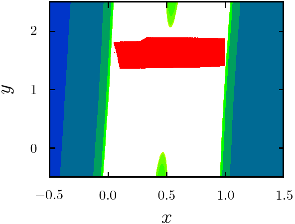
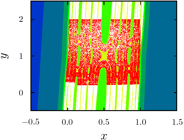
  (a)     (b)     (c)  

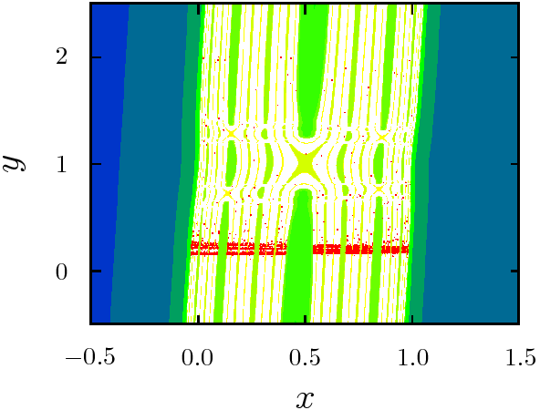
Figure 7: The change of the structure of the invariant chaotic set (red dots) when the attractor undergoes crisis. The colour coding indicates initial conditions arriving at the laminar fixed point in at most $10$ iterations. The tenth iteration of points which have not yet reached the laminar fixed point after $40$ iterations are indicated by red boxes. Parameter values are $a=4.0$ and $\epsilon=0.03$ for all panels, while $\gamma$ takes on different values: (a) $\gamma=0.2$ immediately before the transition from the attractor to the saddle, (b) $\gamma=3$, and (c) $\gamma=6$.

5.2 Parameter dependence of the lifetime for initial conditions on the $y$ axis

A useful and experimentally accessible indicator for the boundaries and their dynamics are lifetimes of perturbations. figure 7 shows the lifetimes for fixed parameters and a two-dimensional domain of different initial conditions. The frequently used lifetime plots for turbulence transitions differ from this one in that they usually show the deviations for a combination of one coordinate (the amplitude of a velocity field) and a parameter (the Reynolds number).

To gain insight into the relation between these two kinds of lifetime plots we first consider the conceptually simplest case where the lifetime of trajectories starting on the $y$ axis is plotted as a function of $a$ and $y$ (figure 8). The large blue domain in the upper half indicates parameters and initial conditions that are quickly attracted to the fixed point. The large red region in the lower left indicates initial conditions which never get to the laminar fixed point, since the turbulent domain is an attractor.

The magnification figure 8(b) focusses on the fuzzy regions in the lifetime plot for $a\simeq 1.25$. As we have seen in figure 5 the boundary between the two coexisting attractors in the coordinate space $(x,y)$ is rough for these parameters. As a consequence the $y$-axis repeatedly crosses the boundary between the domains of attraction of the respective attractors. This gives rise to the observed spiky structure of the interface in the $a$-$y$ plot figure 8(b). Beyond $a\simeq 1.6$ the basin boundary is smooth [figure 5(c,d)], and also in an $a$-$y$-plot there is a sharp boundary between the two domains. It is located close to $y\simeq 0.82$.

When the attractor undergoes the boundary crisis at $a_{cr}=3.93$ the fingers from figure 7 are visible also in the $a$-$y$-plot. They form a hierarchical structure of regions that are mapped into the crisis region and subsequently rapidly approach the laminar state. Note that, when sufficiently resolved, also in this case all fingers extend to the critical parameter value $a_{cr}\simeq 3.93$.

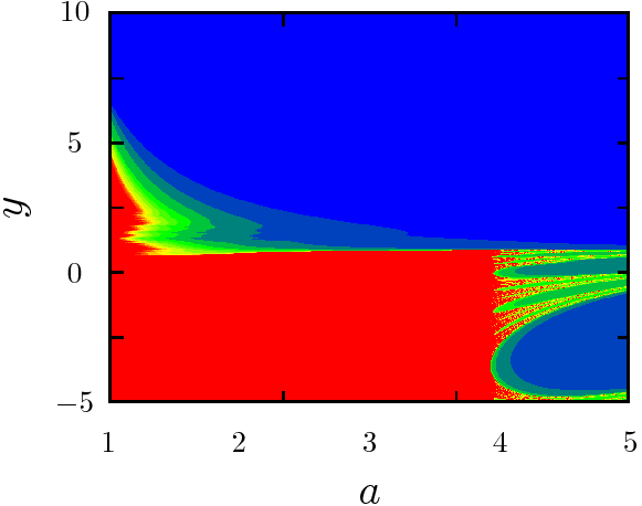
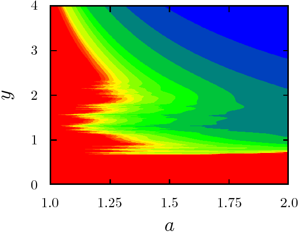
  (a)     (b)     (c)  

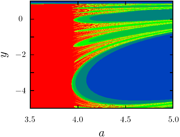
Figure 8: Metamorphosis of the $x=0$ section through the boundary for fixed $\gamma=3.0$, $\epsilon=0.03$, and varying $a$. Panel (a) gives an overview, (b) a blow-up of the region with a rough basin boundary, and (c) focusses on the transition of the chaotic attractor to a chaotic saddle. The colour coding is the same as in figure 5; vertical sections through the present plots exactly agree with a section along the $y$ axis of the corresponding plot in figure 5.

5.3 Generic parameter-coordinate dependence of the lifetime

In figure 8 we chose a section aligned almost parallel to the edge of chaos. On the other hand, in the applications [darbyshire95, Sku06, Sch07a] the amplitude of a perturbation of the laminar state is varied, i.e., initial conditions are chosen along a line extending from the laminar fixed point towards the phase-space domain admitting chaotic motion. Such a line intersects the boundary more or less perpendicularly. In that case one encounters a sharp, smoothly varying boundary between the laminar and turbulent regions for all values below the crisis: It is no longer possible to resolve the roughness of the boundary close to $a\simeq 1.25$. In view of this we focus on the region close to the crisis. The appropriate parts of the parameter plots for four different slopes $m$ of the line

$$y=2+m\;(x+2)$$ (1bfk)

are shown in figure 9.

All panels of figure 9 show hierarchical organised traces of the fingers that we also saw in figure 8(c). This shows that folded and hierarchically organised structures in lifetime-plots are generic. They do not dependent on the specific direction along which initial conditions are chosen. On the other hand the choices differ in the detailed structure of the folds: Figure 9(a) shows the situation where the initial conditions on the line approach the saddle, but do not intersect it. In this case the folds are nicely aligned, and they extend down to different parameter values $a$ well below the bifurcation. After all [cf. figure 7(a)], the fingers invade the domain of attraction before they collide with the attractor at the crisis, and the tips of the finer fingers come down at a later time. Figure 9(b) corresponds to the situation where the line touches the outer edge of the saddle. Consequently, it is exactly along this line that all finger tips simultaneously collide with the attractor. Before the crisis, all initial conditions proceed into the attractor, and at the crisis there is a fractal set of folds with initial conditions escaping to the laminar state appearing all at once. Subsequently, only the scaling of the width of the folds, and hence the fractal dimension of the remaining saddle changes. In figure 9(c) the initial conditions giving rise to chaotic motion lie right in the heart of the chaotic invariant set. In this case the folds also appear simultaneously at the crisis. A new feature is that the internal dynamics of the saddle gives rise to a non-trivial bending of the folds. For many values of $x$, in particular $x=0.5$, there is not a unique value of $a$ which separates regions of persistent chaotic motion for smaller $a$ from a decay to the laminar state. Rather, there can be multiple switching between these possibilities as $a$ is increased. When the line (1bfk) intersects the chaotic set only at its lower boundary [figure 9(d)] the qualitative features of the position-parameter plot are the same as in case (c), except that the multiple switching is less pronounced.

In all cases the observed structure of folded hierarchical tongues are reminiscent of the observations in studies of minimal perturbation amplitudes in pipe flow [darbyshire95, Sch07a]. Thus, this model provides further support for the idea that transient turbulent motion is generated by a chaotic saddle that coexists with a laminar fixed point in the state space of linearly stable shear flows. The following section discusses in more detail the implications of these findings to the transition to turbulence in linearly stable shear flows.

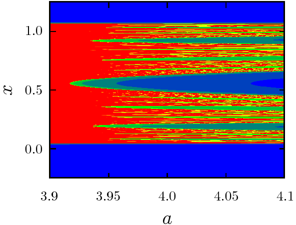
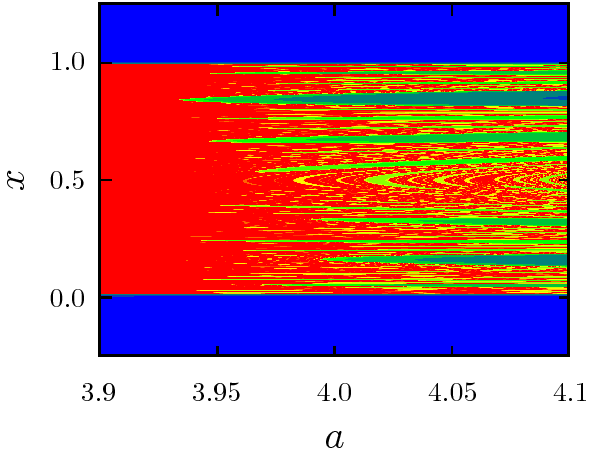
  (a)   (b)
  (c)   (d)

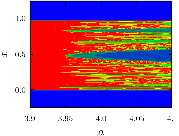
Figure 9: Metamorphosis of a section through the boundary where the coordinates are varied along a line (1bfk). The different panels correspond to (a) $m=1/3$, (b) $m=0$, (c) $m=-1/3$, and (d) $m=-2/3$, respectively. All other parameters and the colour coding are the same as in figure 8.

6 Discussion

6.1 Methods

We have suggested a low-dimensional model in which we can analyse methods and concepts that recently been used in the framework of fluid-mechanical systems [TohItano1999, Sku06, Sch07a, SchneiderGibson2007, DuguetWillisKerswell2007, Viswanath2007, ViswanathCvitanovic2008]. The familiar concept of basin boundaries that separate different attractors was extended to the situation of a saddle coexisting with an attractor. We showed that the orbits defining the basin boundary are a set that changes smoothly when crossing a crisis point where one of the attractors looses its stability. Beyond crisis we denote the closure of this set as the edge of chaos. The edge can be tracked by an iterative algorithm that exploits local properties only and hence can be used both in the situation of co-existing attractors as well as transient chaos coexisting with an attractor, see figure 6(a,right panel).

A standard procedure to determine the basin boundary is backward-iteration. It is more efficient than the direct forward sampling of phase space which was used to generate figure 5. The effort of backward iteration to determine a boundary of box-counting dimension $D_{B}$ with a resolution $\epsilon$ scales like $\epsilon^{-D_{B}}$. In contrast, the direct iteration scales quadratically with the resolution, i.e., like $\varepsilon^{-2}$. The edge tracking algorithm adopted in the present work (figure 6) roughly requires the same numerical effort as backward iteration of the boundary of the region, and it has the additional benefit that beyond the crisis it focusses on the dynamically most relevant region of the edge of chaos while the backward iteration also tracks the circumference of all fingers shown in figure 7.

6.2 Geometry of the boundary

The geometry of the boundary separating laminar and turbulent dynamics can be studied in lifetime plots, where lifetime of initial conditions is either analysed for fixed parameters as a function of state-space coordinates, or by varying a parameter and a coordinate.

For fixed parameters the separating boundary can be smooth or rough. The analysis in section 4.2 shows that roughness can be observed only if (a) the dynamics in the edge is chaotic, and (b) the Lyapunov exponent characterising the chaotic dynamics in the boundary is larger than the one in perpendicular direction. Roughness of the boundary hence is an indicator that there is a strong chaotic dynamics in the basin boundary. Since there is no a priori reason why the Lyapunov exponent pointing out of the separating boundary should be large, it will be interesting to identify a fluid mechanical realization of rough basin boundaries. Ideally, the system should have a control parameter that influences the ratio of the Lyapunov exponents in the longitudinal and transverse directions. A good candidate might be Taylor-Couette flow between independently rotating cylinders with a narrow gap, in which case it is close to the planar shear flows mentioned earlier [Faisst]. But it might also be possible to find evidence for rough boundaries in other parameter regions and geometries where a multitude of attractors can coexist [Abshagen2005].

We have shown here how features of the boundary in the phase space relate to features in the parameter-coordinate space. The latter representation is typically studied in hydrodynamic systems where the Reynolds number Re is adopted as parameter. Increasing Re the boundary shows folded hierarchical organised tongue-like structures. In our model they appear shortly before or at the parameters of the boundary crisis of the turbulent attractor. The tongues have thus been related to the emergence of dynamical connections RempelChianMacauRosa2004acf. between the relative attractor on the edge of chaos and the attractor mimicking stable turbulent motion. These fingers result from the chaotic motion of the attractor undergoing a crisis. The presence of similar tongue-like structures in linearly stable shear flows [darbyshire95, Moe04a, Moe04, Sch07a] further supports the idea of a turbulence generating chaotic saddle in these flows. The long persistence of turbulent motion, i.e., its tiny decay rate, may then be interpreted as another manifestation of supertransients [LaiWinslow1995, BrebanNusse2006].

The local attractor embedded in the separating boundary – the edge state is an object both of theoretical and practical interest. The model shows that the local attractor can be a fixed point, a periodic orbit or a chaotic set. The type of dynamics in the boundary can be chosen independently of whether turbulent motion is generated by an attractor or a saddle. Thus, it is not a priori clear which type of edge state one should expect in transitional shear flows. A chaotic edge state has been identified in pipe flow [Sch07a], and a simple fixed point in plane Couette flow [SchneiderGibson2007]. However, based on our present model we expect that other flow geometries show edge states with various other types of dynamics.

6.3 Outlook

The iterated edge tracking algorithm can be used to analyse any dynamical system showing two coexisting types of dynamics [cassak2007]. Without additional input the method can be used to analyse the position of the boundary and of trajectories in the boundary. A promising future application might be in control strategies, where the edge tracking is used to identify target states for chaos control [Schuster1999]. In various technological applications one is interested to intentionally induce turbulence or keep the flow laminar [Bewley2001, Hoegberg2003, Kawahara2005, Fransson2006, WangGibsonWaleffe2007]. Up to now the setting up of the required effective control mechanisms mostly relies on empirical strategies, long-term experience and intuition. The edge tracking mechanism can provide additional guidance by identifying flow structures on which actuators could focus.

6.4 Closing remarks

The concept of the edge of chaos provides a powerful framework to analyse nonlinear dynamical systems where attractors coexist with a chaotic saddle and where the traditional concept of basin boundaries can no longer be applied. The approach still works for systems with several positive Lyapunov exponents. In that situation it provides insight into local attractors in the edge of chaos.

References

References

- [1] \harvarditemAbshagen et al.2005Abshagen2005 Abshagen J, Lopez J M, Marques F \harvardand Pfister G 2005 J. Fluid Mech. 540, 269–299.
- [2] \harvarditemAshwin et al.1996AshwinBuescuStewart1996 Ashwin P, Buescu J \harvardand Stewart I 1996 Nonlinearity 9, 703–737.
- [3] \harvarditemAshwin et al.2004AshwinRucklidgeSturman2004 Ashwin P, Rucklidge A M \harvardand Sturman R 2004 Chaos 14(3), 571.
- [4] \harvarditemBenet et al.2005BenetBrochMerloSeligman2005 Benet L, Broch J, Merlo O \harvardand Seligman T H 2005 Phys. Rev. E 71, 036225.
- [5] \harvarditemBewley et al.2001Bewley2001 Bewley T, Moin P \harvardand Temam R 2001 J. Fluid Mech. 447, 179–225.
- [6] \harvarditemBottin et al.1997bead_bottin1 Bottin S, Dauchot O \harvardand Daviaud F 1997 Phys. Rev. Lett. 79, 4377–4380.
- [7] \harvarditemBottin et al.1998bead_bottin2 Bottin S, Dauchot O, Daviaud F \harvardand Manneville P 1998 Phys. Fluids 10, 2597–2607.
- [8] \harvarditemBreban \harvardand Nusse2006BrebanNusse2006 Breban R \harvardand Nusse H E 2006 Europhys. Lett. 76, 1036–1042.
- [9] \harvarditemBrosa1991brosa91 Brosa U 1991 Z. Naturforsch. 46a, 473.
- [10] \harvarditemCassak et al.2007cassak2007 Cassak PA, Drake JF, Shay MA \harvardand Eckhardt B 2007 Phys. Rev. Lett., 98, 215001.
- [11] \harvarditemClever \harvardand Busse1997Cle97 Clever R \harvardand Busse F H 1997 J. Fluid Mech. 344, 137–153.
- [12] \harvarditemDarbyshire \harvardand Mullin1995darbyshire95 Darbyshire A G \harvardand Mullin T 1995 J. Fluid Mech. 289, 83–114.
- [13] \harvarditemDellnitz et al.1995DellnitzFieldGolubitskyHohmannMa1995 Dellnitz M, Field M, Golubitsky M, Hohmann A \harvardand Ma J 1995 Int. J. Bifurcation Chaos Appl. Sci. Eng. 5, 1243–1247.
- [14] \harvarditemDevaney2003Devaney2003 Devaney R L 2003 Introduction to Chaotic Dynamical Systems Westview Press Boulder, Colorado.
- [15] \harvarditemDuguet et al.2007DuguetWillisKerswell2007 Duguet Y, Willis A P \harvardand Kerswell R R 2007 arXiv:0711.2175.
- [16] \harvarditemEckhardt et al.2002Eck02 Eckhardt B, Faisst H, Schmiegel A \harvardand Schumacher J 2002 in I. P Castro, P. E Hancock \harvardand T. G Thomas, eds, ‘Advances in Turbulence IX’ CIMNE (Barcelona), 701–708.
- [17] \harvarditemEckhardt et al.2007Eck07b Eckhardt B, Schneider T M, Hof B \harvardand Westerweel J 2007 Annu. Rev. Fluid Mech. 39, 447–468.
- [18] \harvarditemEckhardt2008Eckh08 Eckhardt B 2008 Nonlinearity 21, T1–T11.
- [19] \harvarditemEckhardt et al.2008aberdeen Eckhardt B, Holger F, Schmiegel A \harvardand Schneider T M 2008 Phil. Trans. A. Roy. Soc. (London) A 366, 1297–1315.
- [20] \harvarditemFaisst \harvardand Eckhardt2000Faisst Faisst H \harvardand Eckhardt E 2000, Phys. Rev. E 61, 7227–7230.
- [21] \harvarditemFaisst \harvardand Eckhardt2003Fai03 Faisst H \harvardand Eckhardt B 2003 Phys. Rev. Lett. 91, 224502.
- [22] \harvarditemFaisst \harvardand Eckhardt2004FE04 Faisst H \harvardand Eckhardt B 2004 J. Fluid Mech. 504, 343–352.
- [23] \harvarditemFransson et al.2006Fransson2006 Fransson J H M, Talamelli A, Brandt L \harvardand Cossu C 2006 Phys. Rev. Lett. 96, 064501.
- [24] \harvarditemFujisaka \harvardand Yamada1983FujisakaYamada1983 Fujisaka H \harvardand Yamada T 1983 Prog. Theor. Phys. 69, 32.
- [25] \harvarditemGrebogi et al.1987GrebogiOttRomeirasYorke1987 Grebogi C, Ott E, Romeiras F \harvardand Yorke J A 1987 Phys. Rev. A 36(11), 5365–5380.
- [26] \harvarditemGrebogi et al.1982greb82 Grebogi C, Ott E \harvardand Yorke J A 1982 Phys. Rev. Lett. 48, 1507–1510.
- [27] \harvarditemGrebogi et al.1983aGrebogiOttYorke1983 Grebogi C, Ott E \harvardand Yorke J A 1983a Physica D 7(1-3), 181–200.
- [28] \harvarditemGrebogi et al.1983bGrebogiOttYorke1983PRL Grebogi C, Ott E \harvardand Yorke J A 1983b Phys. Rev. Lett. 50(13), 935–938; 51(10), 942 (erratum).
- [29] \harvarditemGrossmann2000grossmann00 Grossmann S 2000 Rev. Mod. Phys. 72, 603–618.
- [30] \harvarditemGu et al.1984GuTungYuanFengNarducci1984 Gu Y, Tung M, Yuan J M, Feng D H \harvardand Narducci L M 1984 Phys. Rev. Lett. 52(9), 701–704.
- [31] \harvarditemHof et al.2006Hof06 Hof B, Westerweel J, Schneider T M \harvardand Eckhardt B 2006 Nature 443, 60–64.
- [32] \harvarditemHögberg et al.2003Hoegberg2003 Högberg M, Bewley T \harvardand Henningson D 2003 J. Fluid Mech. 481, 149–175.
- [33] \harvarditemHu \harvardand Yang2002HuYang2002 Hu B \harvardand Yang H 2002 Phys. Rev. E 65(6), 066213.
- [34] \harvarditemHunt et al.1997Hunt97 Hunt B R, Ott E \harvardand Yorke J A 1997 Phys. Rev. E 55, 4029–4034.
- [35] \harvarditemKapitaniak et al.1999KapitaniakLaiGrebogi1999 Kapitaniak T, Lai Y C \harvardand Grebogi C 1999 Phys. Lett. A 259(6), 445–450.
- [36] \harvarditemKapitaniak et al.2003KapitaniakMaistrenkoGrebogi2003 Kapitaniak T, Maistrenko Y \harvardand Grebogi C 2003 Chaos, Solitons and Fractals 17(1), 61–66.
- [37] \harvarditemKawahara2005Kawahara2005 Kawahara G 2005 Phys. Fluids 17(4), 041702.
- [38] \harvarditemKerswell2005Ker05 Kerswell R R 2005 Nonlinearity 18, R17–R44.
- [39] \harvarditemKim et al.2003KimLimOttHunt2003 Kim S Y, Lim W, Ott E \harvardand Hunt B 2003 Phys. Rev. E 68(6), 066203.
- [40] \harvarditemKovács \harvardand Wiesenfeld2001KovacsWiesenfeld2001 Kovács Z \harvardand Wiesenfeld L 2001 Phys. Rev. E 63(5), 056207.
- [41] \harvarditemLai2001Lai2001 Lai Y C 2001 Physica D 150, 1–13.
- [42] \harvarditemLai \harvardand Winslow1995LaiWinslow1995 Lai Y C \harvardand Winslow R L 1995 Phys. Rev. Lett. 74(26), 5208–5211.
- [43] \harvarditemMaistrenko et al.1998MaistrenkoMaistrenkoPopovichMosekilde1998 Maistrenko Y L, Maistrenko V L, Popovich A \harvardand Mosekilde E 1998 Phys. Rev. E 57(3), 2713–2724.
- [44] \harvarditemMoehlis et al.2004aMoe04a Moehlis J, Eckhardt B \harvardand Faisst H 2004a CHAOS 14, S11.
- [45] \harvarditemMoehlis et al.2004bMoe04 Moehlis J, Faisst H \harvardand Eckhardt B 2004b New J. Phys. 6, 56.
- [46] \harvarditemMullin \harvardand Peixinho2006aMul05 Mullin T \harvardand Peixinho J 2006a in ‘IUTAM Symposium on laminar-turbulent transition’ Springer Bangalore, 45–56.
- [47] \harvarditemMullin \harvardand Peixinho2006bMul06 Mullin T \harvardand Peixinho J 2006b J. Low Temp. Phys. 145, 75–88.
- [48] \harvarditemNagata1990Nag90 Nagata M 1990 J. Fluid Mech. 217, 519–527.
- [49] \harvarditemNagata1997Nag97 Nagata M 1997 Phys. Rev. E 55, 2023–2025.
- [50] \harvarditemOsinga2006Osinga2006 Osinga H M 2006 Phys. Rev. E 74, 035201(R).
- [51] \harvarditemOtt2002Ott2002 Ott E 2002 Chaos in Dynamical Systems Cambridge University Press.
- [52] \harvarditemPazó \harvardand Matías2005PazoMatias2005 Pazó D \harvardand Matías M A 2005 Europhys. Lett. 72(2), 176–182.
- [53] \harvarditemPeitgen \harvardand Richter2000peitgen Peitgen H O \harvardand Richter P H 2000, The beauty of fractals, Springer
- [54] \harvarditemPeixinho \harvardand Mullin2006Pei06 Peixinho J \harvardand Mullin T 2006 Phys. Rev. Lett. 96, 094501.
- [55] \harvarditemPeixinho \harvardand Mullin2007Pei07 Peixinho J \harvardand Mullin T 2007 J. Fluid Mech. 582, 169–178.
- [56] \harvarditemPikovsky \harvardand Grassberger1991PikovskyGrassberger1991 Pikovsky A \harvardand Grassberger P 1991 J. Phys. A 24(19), 4587–4597.
- [57] \harvarditemPikovsky et al.2001PikovskyRosenblumKurths2001 Pikovsky A, Rosenblum M \harvardand Kurths J 2001 Synchronization: A Universal Concept in Nonlinear Sciences Cambridge University Press Cambridge.
- [58] \harvarditemPringle \harvardand Kerswell2007Pri07 Pringle C \harvardand Kerswell R R 2007 Phys. Rev. Lett. 99, 074502.
- [59] \harvarditemRempel et al.2004RempelChianMacauRosa2004a Rempel E L, Chian A C L, Macau E E \harvardand Rosa R R 2004 Physica D 199(3-4), 407–424.
- [60] \harvarditemRobert et al.2000RobertAlligoodOttYorke2000 Robert C, Alligood K T, Ott E \harvardand Yorke J A 2000 Physica D 144(1-2), 44–61.
- [61] \harvarditemRössler1983Roessler1983 Rössler O E 1983 Z. Naturforsch. 38a, 788–801.
- [62] \harvarditemRosa and Ott1999Rosa1999 Rosa E and Ott E 1999, Phys. Rev. E 59, 343–352.
- [63] \harvarditemSchneider et al.2007Sch07a Schneider T M, Eckhardt B \harvardand Yorke J A 2007 Phys. Rev. Lett. 99, 034502.
- [64] \harvarditemSchneider et al.2008SchneiderGibson2007 Schneider T M, Gibson J F, Lagha M, De Lillo F \harvardand Eckhardt B 2008 Phys. Rev. E (in press).
- [65] \harvarditemSchneider \harvardand Eckhardt2008aSchn08b Schneider T M \harvardand Eckhardt B 2008a Phys. Rev. E (in press).
- [66] \harvarditemSchneider \harvardand Eckhardt2008bSchneiderEckhardt2008 Schneider T M \harvardand Eckhardt B 2008b Phil. Trans. Roy. Soc. A (submitted).
- [67] \harvarditemSchuster1999Schuster1999 Schuster H 1999 Handbook of chaos control Wiley-VCH, Weinheim.
- [68] \harvarditemSkufca et al.2006Sku06 Skufca J D, Yorke J A \harvardand Eckhardt B 2006 Phys. Rev. Lett. 96, 174101.
- [69] \harvarditemTél1988tel1988 Tél T 1988 Z. Naturforsch. 43a, 1154–1174.
- [70] \harvarditemTél1990tel1990 Tél T 1990 in H Bai-lin, ed., ‘Directions in Chaos Vol. 3: Experimental Study and Characterization of Chaos’ World Scientific Singapore, 149–211.
- [71] \harvarditemTél \harvardand Lai2008TelLai2008 Tél T \harvardand Lai Y C 2008 Phys. Rep. 460(6), 245–275.
- [72] \harvarditemToh \harvardand Itano1999TohItano1999 Toh S \harvardand Itano T 1999 arXiv:physics/9905012.
- [73] \harvarditemViswanath2007Viswanath2007 Viswanath D 2007 arXiv:physics/0701337.
- [74] \harvarditemViswanath \harvardand Cvitanovic2008ViswanathCvitanovic2008 Viswanath D \harvardand Cvitanovic P 2008 arXiv:0801.1918.
- [75] \harvarditemWaalkens et al.2004WaalkensBurbanksWiggins2004 Waalkens H, Burbanks A \harvardand Wiggins S 2004 J. Phys. A 37, L257–L265.
- [76] \harvarditemWaleffe2003Wal03 Waleffe F 2003 Phys. Fluids 15, 1517–1534.
- [77] \harvarditemWang et al.2007WangGibsonWaleffe2007 Wang J, Gibson J \harvardand Waleffe F 2007 Phys. Rev. Lett. 98, 204501.
- [78] \harvarditemWedin \harvardand Kerswell2004TW_bristol Wedin H \harvardand Kerswell R R 2004 J. Fluid Mech. 508, 333–371.
- [79] \harvarditemWiggins et al.2001WigginsWiesenfeldJaffeUzer2001 Wiggins S, Wiesenfeld L, Jaffé C \harvardand Uzer T 2001 Phys. Rev. Lett. 86(24), 5478–5481.
- [80] \harvarditemYamada \harvardand Fujisaka1983YamadaFujisaka1983 Yamada T \harvardand Fujisaka H 1983 Prog. Theor. Phys. 69(1), 32–47.
- [81]