Y-junction of superconducting Josephson chains

Abstract

We show that, for pertinent values of the fabrication and control parameters, an attractive finite coupling fixed point emerges in the phase diagram of a Y-junction of superconducting Josephson chains. The new fixed point arises only when the dimensionless flux $f$ piercing the central loop of the network equals $\pi$ and, thus, does not break time-reversal invariance; for $f\neq\pi$, only the strongly coupled fixed point survives as a stable attractive fixed point. Phase slips (instantons) have a crucial role in establishing this transition: we show indeed that, at $f=\pi$, a new set of instantons -the W-instantons- comes into play to destabilize the strongly coupled fixed point. Finally, we provide a detailed account of the Josephson current-phase relationship along the arms of the network, near each one of the allowed fixed points. Our results evidence remarkable similarities between the phase diagram accessible to a Y-junction of superconducting Josephson chains and the one found in the analysis of quantum Brownian motion on frustrated planar lattices.

1 Introduction

Networks of fermionic and bosonic quantum systems are now attracting increased attention, due to their relevance to the engineering of electronic and spintronic nanodevices. Recently, in Ref.[1], the transport properties of a Y-junction composed of three quantum wires enclosing a magnetic flux were studied: modeling the wires as Tomonaga-Luttinger liquids (TLL), the authors of Ref.[1] were able to show the existence of an attractive fixed point, characteristic of the network geometry of the circuit. A repulsive finite coupling fixed point has been found in Ref.[2], in the analysis of Y-junctions of one-dimensional Bose liquids.

Crossed TLL’s are the subject of several recent analytical [3], as well as numerical [4] papers: these analyses show that, in crossed TLL’s, a junction induces behaviors similar to those arising from impurities in condensed matter systems. In Ref.[5] it has been pointed out that, in crossed spin-1/2 Heisenberg chains, novel critical behaviors emerge since, as a result of the crossing, some operators turn from irrelevant to marginal, leading to correlation functions exhibiting power-law decays with nonuniversal exponents.

Impurity models have been largely studied, in connection with the Kondo models [6], with magnetic chains [7], and for describing static impurities in TLL’s [8]. A renormalization group approach to those systems leads, after bosonization [9], to the investigation of the phases accessible to pertinent boundary sine-Gordon models [8]. Scattering from an impurity often leads the boundary coupling strength to scale to the strongly coupled fixed point (SFP),which is rather simple since it describes a fully screened spin in the Kondo problem or a severed chain in the Kane-Fisher model [10]. A remarkable exception is provided by the fixed point attained in the overscreened Kondo problem, where an attractive finite coupling fixed point (FFP) emerges in the phase diagram [6]. The FFP is usually characterized by novel nontrivial universal indices and by specific symmetries.

Superconducting Josephson devices provide remarkable realizations of quantum systems with impurities [11, 12]. For superconducting Josephson chains with an impurity in the middle [13, 11] or for SQUID devices [14, 12] the phase diagram admits only two fixed points: an unstable weakly coupled fixed point (WFP), and a stable one at strong coupling. The boundary field theory approach developed in Ref.[11, 12] not only allows for an accurate determination of the phases accessible to a superconducting device, but also for a field-theoretical treatment of the phase slips (instantons), describing quantum tunneling between degenerate ground-states; furthermore, it helps to evidence remarkable analogies with models of quantum Brownian motion on frustrated planar lattices [15, 16].

In this paper, we show that, for pertinent values of the fabrication and control parameters, a FFP emerges in a Y-shaped Josephson junction network (YJJN); then, we probe the behavior of the YJJN near this fixed point by computing the Josephson current along the arms of the network. The paper is organized as follows:

In section 2 we provide a Luttinger liquid description of the YJJN and derive the boundary effective Hamiltonian describing the network;

In section 3 we investigate the fixed points accessible to a YJJN for different values of the Luttinger parameter $g$ and of the magnetic field threading the central loop of the YJJN;

Section 4 is devoted to the computation of the current-phase relation of the Josephson currents along the three arms of the YJJN, with the purpose of determining the current’s pattern near the fixed points found in section 3. There we evidence the remarkably different effects of phase slips near the SFP and the FFP;

In section 5 we argue that -as it happens with other superconducting devices [17] - a YJJN allows to engineer an effective coherent two-level quantum system, whose states are characterized by two different macroscopic current’s patterns along its arms;

Section 6 is devoted to our concluding remarks, while the appendices provide the necessary background for the derivation presented in the paper.

2 Effective Hamiltonian of a YJJN

The $Y$-shaped Josephson junction network we consider is shown in Fig.1. It is made with three finite Josephson junction (JJ) chains ending on one side (inner boundary) with a weak link of nominal strength $\lambda$ and on the other side (outer boundary) by three bulk superconductors held at phases $\varphi_{j}$ ($j=1,2,3$). The three chains are connected by the weak links to a circular JJ chain C, pierced by a dimensionless magnetic flux $f$. For simplicity, we assume that all the junctions have Josephson energies $E_{J}$ and $\lambda\ll E_{J}$. The Hamiltonian describing the central region, $H_{\bf C}$, is given by

$$H_{\bf C}=\frac{E_{c}}{2}\sum_{i=1}^{3}\left[-i\frac{\partial}{\partial\phi_{0}^{(i)}}-{\bf N^{\prime}}\right]^{2}-\frac{E_{J}}{2}\sum_{i=1}^{3}[e^{i[\phi_{0}^{(i)}-\phi_{0}^{(i+1)}+\frac{f}{3}]}+e^{-i[\phi_{0}^{(i)}-\phi_{0}^{(i+1)}+\frac{f}{3}]}]\>\>\>\>,$$ (1)

where $E_{c}$ is the charging energy of each grain, ${\bf N^{\prime}}$ is the gate voltage applied to the i^th junction, and $\phi_{0}^{(i)}$ ($i=1,2,3;i+3\equiv i$) is the phase of the superconducting order parameter at the $i$-th grain in C.

Figure 1: $Y$-shaped Josephson junction network: all the junctions are equal to each other and have nominal Josephson energy $E_{J}$, except for the three ones connecting the central region to the endpoints of the chain, that have nominal energy $\lambda$.

Following a standard procedure [13, 11, 12], the Hamiltonian in Eq.(1) can be presented as

$$H_{\bf C}=-\tilde{H}\sum_{i=1}^{3}[S_{0}^{(i)}]^{z}-\frac{E_{J}}{2}\sum_{i=1}^{3}\{e^{i\frac{f}{3}}[S_{0}^{(i)}]^{+}[S_{0}^{(i+1)}]^{-}+e^{-i\frac{f}{3}}[S_{0}^{(i+1)}]^{+}[S_{0}^{(i)}]^{-}\}\>\>\>\>,$$ (2)

with $\tilde{H}\propto E_{c}$, $[S_{0}^{(i)}]^{z}=n^{(i)}_{0}-{\bf N^{\prime}}-\frac{1}{2}$ and $[S_{0}^{(i)}]^{\pm}=e^{\pm i\phi_{0}^{(i)}}$, where $n^{(i)}_{0}$ is the total charge at grain $i$ (measured in units of $e^{*}$).

For $\tilde{H}>E_{J}>0$, the eigenstates of Eq.(2) are given by

• A “fully polarized” ground state:

  $|0\rangle=|\uparrow\uparrow\uparrow\rangle$, with energy $\epsilon_{0}=-\frac{3}{2}\tilde{H}$;

• A low-energy triplet of states:

  $|1,1\rangle=\frac{1}{\sqrt{3}}[|\downarrow\uparrow\uparrow\rangle+|\uparrow\downarrow\uparrow\rangle+|\uparrow\uparrow\downarrow\rangle]$, with energy $\epsilon_{1,1}(f)=-\frac{\tilde{H}}{2}-E_{J}\cos(\frac{f}{3})$;

  $|1,2\rangle=\frac{1}{\sqrt{3}}[|\downarrow\uparrow\uparrow\rangle-e^{-i\frac{\pi}{3}}|\uparrow\downarrow\uparrow\rangle-e^{i\frac{\pi}{3}}|\uparrow\uparrow\downarrow\rangle]$, with energy $\epsilon_{1,2}(f)=-\frac{\tilde{H}}{2}-E_{J}\cos(\frac{f-\pi}{3})$;

  $|1,3\rangle=\frac{1}{\sqrt{3}}[|\downarrow\uparrow\uparrow\rangle-e^{i\frac{\pi}{3}}|\uparrow\downarrow\uparrow\rangle-e^{-i\frac{\pi}{3}}|\uparrow\uparrow\downarrow\rangle]$, with energy $\epsilon_{1,3}(f)=-\frac{\tilde{H}}{2}-E_{J}\cos(\frac{f+\pi}{3})$;

• A high-energy triplet of states:

  $|2,1\rangle=\frac{1}{\sqrt{3}}[|\downarrow\downarrow\uparrow\rangle+|\downarrow\uparrow\downarrow\rangle+|\uparrow\downarrow\downarrow\rangle]$, with energy $\epsilon_{2,1}(f)=\frac{\tilde{H}}{2}-E_{J}\cos(\frac{f}{3})$;

  $|2,2\rangle=\frac{1}{\sqrt{3}}[|\uparrow\downarrow\downarrow\rangle-e^{i\frac{\pi}{3}}|\downarrow\uparrow\downarrow\rangle-e^{-i\frac{\pi}{3}}|\downarrow\downarrow\uparrow\rangle]$, with energy $\epsilon_{2,2}(f)=\frac{\tilde{H}}{2}-E_{J}\cos(\frac{f-\pi}{3})$;

  $|2,3\rangle=\frac{1}{\sqrt{3}}[|\uparrow\downarrow\downarrow\rangle-e^{-i\frac{\pi}{3}}|\downarrow\uparrow\downarrow\rangle-e^{i\frac{\pi}{3}}|\downarrow\downarrow\uparrow\rangle]$, with energy $\epsilon_{3,2}(f)=\frac{\tilde{H}}{2}-E_{J}\cos(\frac{f+\pi}{3})$;

• A high-energy fully-polarized state $|3\rangle=|\downarrow\downarrow\downarrow\rangle$, with energy $\epsilon_{3}=3\tilde{H}$.

We require that C is connected to the three finite chains via a charge tunneling Hamiltonian $H_{T}$, given by

$$H_{T}=-\lambda\sum_{i=1}^{3}\cos[\phi_{1}^{(i)}-\phi_{0}^{(i)}]\;\;\;\;.$$ (3)

Since $\lambda/E_{J}\ll 1$, one may resort to a Schrieffer-Wolff transformation [18], to derive an Hamiltonian $H_{B}$ describing the effective boundary interaction at the inner boundaries of the three chains. To the second order in $\lambda$, $H_{B}$ is given by

$$H_{B}\approx B(f)\sum_{i=1}^{3}e^{-i\phi_{1}^{(i)}}e^{i\phi_{1}^{(i)}}+A(f)\sum_{i=1}^{3}e^{-i\phi_{1}^{(i)}}e^{i\phi_{1}^{(i+1)}}+{\rm h.c.}\;\;\;\;,$$ (4)

where $B(f)=\frac{\lambda^{2}}{12}\sum_{k=1}^{3}\left(\frac{1}{\epsilon_{0}-\epsilon_{1,k}(f)}\right)$, and $A(f)=\frac{\lambda^{2}}{12}\sum_{k=1}^{3}\left(\frac{e^{-\frac{2}{3}\pi i(k-1)}}{\epsilon_{0}-\epsilon_{1,k}(f)}\right)$.

$A(f)$ is, in general, a complex number, equal to $-E_{W}e^{i\gamma}$ ($E_{W}>0$). Its phase $\gamma$ is related to the magnetic flux by

$$\tan\gamma=\frac{\sqrt{3}}{2}\left[\frac{\sum_{k=2,3}\frac{(-1)^{k}}{\epsilon_{0}-\epsilon_{1,k}(f)}}{\frac{1}{\epsilon_{0}-\epsilon_{1,1}(f)}-\frac{1}{2}\sum_{k=2,3}\frac{1}{\epsilon_{0}-\epsilon_{1,k}(f)}}\right]\>\>\>\>;$$ (5)

for $f=2k\pi$ and $(2k+1)\pi$ ($k=0,\pm 1,\pm 2,\ldots$), $\gamma=2k\pi/3$ and $(2k+1)\pi/3$, respectively.

The Hamiltonian describing the three finite chains may be written as [13]

$$H_{0}=\frac{E_{c}}{2}\sum_{i=1,2,3}\sum_{j=1}^{L/a}\left[-i\frac{\partial}{\partial\phi_{j}^{(i)}}-{\bf N}\right]^{2}+$$

$$\sum_{i=1,2,3}\sum_{j=1}^{L/a-1}\left[-E_{J}\cos(\phi_{j}^{(i)}-\phi_{j+1}^{(i)})+E^{z}\left(-i\frac{\partial}{\partial\phi_{j}^{(i)}}-{\bf N}\right)\left(-i\frac{\partial}{\partial\phi_{j+1}^{(i)}}-{\bf N}\right)\right]\>\>\>\>.$$ (6)

In Eq.(6) $\phi_{j}^{(i)}$ is the phase of the superconducting order parameter at grain $j$ of the $i$th chain, $-i\frac{\partial}{\partial\phi_{j}^{(i)}}$ is the corresponding charge operator; ${\bf N}$ is proportional to the gate voltage $V_{g}$ applied to each grain, while $L$ and $a$ are the length of each chain and the lattice spacing, respectively. $E^{z}$ accounts for the Coulomb repulsion between charges on nearest neighboring junctions. Following the procedure detailed in appendix A, Eq.(6) may be written in Tomonaga-Luttinger (TL)-form [19] as

$$H_{0}=\sum_{j=1,2,3}\frac{g}{4\pi}\>\int_{0}^{L}\>dx\>\left[\frac{1}{v}\left(\frac{\partial\Phi_{j}}{\partial t}\right)^{2}+v\left(\frac{\partial\Phi_{j}}{\partial x}\right)^{2}\right]\;\;\;\;,$$ (7)

where the fields $\Phi_{j}(x)$ ($j=1,2,3$) describe the collective plasmon modes of the chains, $\Delta=E^{z}-\frac{3}{16}\frac{(E_{J})^{2}}{E_{c}}$, $v=v_{f}\sqrt{1+\frac{4\pi a\Delta[1-\cos(2ak_{f})]}{v_{f}}}$, and $g=\sqrt{\frac{v_{f}}{v_{f}+4\pi a\Delta[1-\cos(2ak_{f})]}}$, with $v_{f}=2\pi E_{J}\sin(ak_{f})$ and $k_{f}={\rm arccos}(hE_{c}/E_{J})$.

Since at the outer boundary the three chains are connected to three bulk superconductors at fixed phases $\varphi_{j}$, the fields $\Phi_{j}$ must satisfy the Dirichlet boundary conditions

$$\Phi_{j}(L)=\sqrt{2}[2\pi n_{j}+\varphi_{j}],$$ (8)

where $j=1,2,3$ and $n_{j}$ are integers. On the inner boundary, the three chains are connected to C via $H_{T}$: as a result, one should impose here Neumann boundary conditions (i.e., $\frac{\partial\Phi_{j}(0)}{\partial x}=0$). For our following analysis, it is most convenient to introduce linear combinations of the plasmon fields, such as $X(x)=\frac{1}{\sqrt{3}}\sum_{j=1}^{3}\Phi_{j}(x)$, $\chi_{1}(x)=\frac{1}{\sqrt{2}}[\Phi_{1}(x)-\Phi_{2}(x)]$, and $\chi_{2}(x)=\frac{1}{\sqrt{6}}[\Phi_{1}(x)+\Phi_{2}(x)-2\Phi_{3}(x)]$. Since $E_{W}$ is of order $\lambda^{2}/E_{J}$, one has that $E_{W}/E_{J}\ll 1$ and, thus, at $x=0$, the fields $\chi_{1},\chi_{2}$ also satisfy Neumann boundary conditions. Of course, at the outer boundary, $\chi_{1},\chi_{2}$ satisfy Dirichlet boundary conditions.

In the long wavelength limit, the first term on the r.h.s. of Eq.(4) may be well approximated as $3B(f)+{\rm const}\frac{\partial X(0)}{\partial x}$. Due to Neumann boundary conditions, this term only contributes by an irrelevant constant to Eq.(4). Eq.(4) may be, then, usefully presented in the form

$$H_{B}=-2\bar{E}_{W}\sum_{i=1}^{3}:\cos[\vec{\alpha}_{i}\cdot\vec{\chi}(0)+\gamma]:\;\;\;\;,$$ (9)

with $\vec{\alpha}_{1}=(1,0)$, $\vec{\alpha}_{2}=(-\frac{1}{2},\frac{\sqrt{3}}{2})$, $\vec{\alpha}_{3}=(-\frac{1}{2},-\frac{\sqrt{3}}{2})$. The colons ($:\>:$) in Eq.(9) denote normal ordering with respect to the vacuum of the bosonic fields $\chi_{1},\chi_{2}$. The effective coupling $\bar{E}_{W}$ is given by $\bar{E}_{W}=\left(\frac{a}{L}\right)^{\frac{1}{g}}E_{W}$. Eq.(9) may be regarded as the bosonic version of the boundary Hamiltonian describing the central region of a $Y$-junction of three quantum wires, introduced in Ref.[1]. As we shall see, setting $\gamma=(2k+1)\pi/3$, allows for the emergence of a new attractive fixed point also in the phase diagram of the $Y$-junction of superconducting Josephson chains. It should be noticed that this fixed point is attractive, since in a superconducting network, bosons are charged; this should be contrasted with the situation arising in $Y$-shaped networks of neutral atomic condensates [2], where the FFP is repulsive.

3 Phase diagram of a YJJN

In this section, we use the renormalization group approach to investigate the phases accessible to a superconducting YJJN. As evidenced in the analysis of other superconducting devices [11, 12], there is usually a range of values of the Luttinger parameter $g$ for which the phase diagram allows for a crossover from an unstable WFP to a stable SFP. For a Josephson chain with an impurity [13, 11] and for SQUID devices [14, 12], the crossover is driven by the ratio $L/L_{*}$, where $L$ is the length of the chain (or the diameter of the superconducting loop in a SQUID) and $L_{*}$ is a pertinently defined healing length [11]. Here, we shall show that, when $\gamma=(2k+1)\pi/3$, a new relevant boundary interaction, emerging in a YJJN at strong coupling, destabilizes the SFP: as a result, since the WFP is IR unstable, an IR stable attractive FFP emerges in the phase diagram. Remarkably, for these values of $\gamma$, the phase diagram of a YJJN is similar to the one accessible to a bosonic quantum Brownian particle on planar frustrated lattices [15], and to spin-1/2 fermions hopping on $Y$-junctions of quantum wires [1].

3.1 The weakly coupled fixed point

Setting $\bar{E}_{W}=0$ defines the WFP, where the fields $\chi_{1}(x),\chi_{2}(x)$ obey Dirichlet boundary conditions at the outer boundary and Neumann boundary conditions at the inner boundary. As a result, the mode expansion of $\chi_{i}$ is given by

$$\chi_{i}(x,t)=\xi_{i}+\sqrt{\frac{2}{g}}\>\sum_{n}\cos\left[\frac{\pi}{L}\left(n+\frac{1}{2}\right)x\right]\frac{\alpha_{i}(n)}{n+\frac{1}{2}}\>e^{-i\frac{\pi}{L}\left(n+\frac{1}{2}\right)vt}\>\>\>\>,$$ (10)

with $[\alpha_{i}(n),\alpha_{j}(n^{\prime})]=\delta_{ij}\left(n+\frac{1}{2}\right)\delta_{n+n^{\prime}-1,0}$, $\xi_{1}=\mu_{1}+2\pi n_{12}$, $\xi_{2}=\mu_{2}+\frac{2}{\sqrt{3}}\left[2\pi n_{13}-\pi n_{12}\right]$, $(\mu_{1},\mu_{2})=([\varphi_{1}-\varphi_{2}],\frac{2}{\sqrt{3}}[(\varphi_{1}-\varphi_{3})-(\varphi_{1}-\varphi_{2})/2])$, with $n_{ij}=n_{i}-n_{j}$.

The perturbative renormalization group equations may be derived from the partition function, written as a power series in the boundary interaction strength. From Eq.(9), one gets

$$\frac{{\bf Z}}{{\bf Z}_{0}}=\sum_{N=0}^{\infty}\bar{E}_{W}^{N}\sum_{\epsilon_{1},\ldots,\epsilon_{N}=\pm 1}\>\exp\left[\sum_{j=1}^{N}\epsilon_{j}\gamma\right]\times$$

$$\int_{0}^{\beta}\>d\tau_{1}\>\int_{0}^{\tau_{1}-\frac{a}{v}}\>d\tau_{2}\>\ldots\>\int_{0}^{\tau_{N-1}-\frac{a}{v}}\>d\tau_{N}\>\langle{\bf T}_{\tau}\prod_{j=1}^{N}:\exp[i\epsilon_{j}\vec{\alpha}_{k_{j}}\cdot\vec{\chi}(\tau_{j})]:\rangle_{0}\>\>\>\>,$$ (11)

with ${\bf Z}_{0}=\prod_{n=0}^{\infty}[1-\bar{q}^{n+\frac{1}{2}}]^{2}$, $\bar{q}=\exp\left[-\beta\frac{\pi v}{L}\right]$), and $\beta=(k_{B}T)^{-1}$. In Eq.(11), the lattice step $a$ has to be regarded as the short-distance cutoff, $\langle\ldots\rangle_{0}$ denotes thermal averages with respect to ${\bf Z}_{0}$, and ${\bf T}_{\tau}$ denotes imaginary time ordered products.

The $N$-point functions of the vertex operators $:\exp[i\epsilon_{j}\vec{\alpha}_{k_{j}}\cdot\vec{\chi}(\tau_{j})]:$ are readily computed using Wick’s theorem for vertex operators [20]. As $\beta v/L\gg 1$, they are given by

$$\langle{\bf T}_{\tau}\prod_{j=1}^{N}:\exp[i\epsilon_{j}\vec{\alpha}_{k_{j}}\cdot\vec{\chi}(\tau_{j})]:\rangle_{0}=\exp\left[\frac{2}{g}\sum_{i<j=1}^{N}\epsilon_{i}\epsilon_{j}\vec{\alpha}_{k_{i}}\cdot\vec{\alpha}_{k_{j}}\>\gamma_{\tau}(\tau_{i},\tau_{j})\right]\>\>\>\>,$$ (12)

with

$$\gamma_{\tau}(\tau,\tau^{\prime})=\ln\left|\frac{e^{\frac{\pi}{2L}v\tau}-e^{\frac{\pi}{2L}v\tau^{\prime}}}{e^{\frac{\pi}{2L}v\tau}+e^{\frac{\pi}{2L}v\tau^{\prime}}}\right|\>\>\>\>.$$ (13)

As a result, at the WFP, one sees that the scaling dimension of the boundary interaction in Eq.(9) is given by $h_{W}(g)=\frac{1}{g}$, and that the dimensionless coupling strength $G(L)=L\bar{E}_{W}$ scales as $G(L)\sim L^{1-\frac{1}{g}}$.

From the operator product expansion (O.P.E.) between vertex operators

$$\left\{:\exp\left[i\vec{\alpha}_{i}\cdot\chi(\tau)\right]::\exp\left[i\vec{\alpha}_{j}\cdot\chi(\tau^{\prime})\right]:\right\}_{\tau^{\prime}\to\tau^{-}}\approx\left[\frac{v(\tau-\tau^{\prime})}{L}\right]^{-\frac{2}{g}}:\exp\left[-i\vec{\alpha}_{k}\cdot\vec{\chi}(\tau)\right]:\;\;\;\;,$$ (14)

with $i\neq j\neq k$, one gets the second-order renormalization group equations for the complex coupling $G(L)e^{i\gamma}$ as

$$\frac{d[G(L)e^{i\gamma}]}{d\ln(\frac{L}{L_{0}})}=[1-\frac{1}{g}][G(L)e^{i\gamma}-2G^{2}(L)e^{-2i\gamma}\;\;\;\;,$$ (15)

which may be usefully presented as

$$\frac{dG(\ell)}{d\ell} = [1-\frac{1}{g}]G(\ell)+2\cos(3\gamma)G^{2}(\ell)$$ (16)

$$\frac{d\gamma}{d\ell} = -2\sin(3\gamma)G^{2}(\ell)\>\>\>\>$$ (17)

( $\ell=\ln\left(\frac{L}{L_{0}}\right)$). Since Eqs.(16,17) are periodic under $\gamma\longrightarrow\gamma+\frac{2\pi}{3}$, the resulting phase diagram of the YJJN will present the same periodicity. Also, the phase diagram strongly depends on whether $g<1$, or $g>1$. Indeed:

1. For $g<1$, the linear term in Eq.(16) has a negative coefficient and, thus, $\forall\gamma$, the system is attracted by a fixed point with $G_{*}=0$. Furthermore, Eq.(17) shows that the value of $\gamma$ at the attractive fixed point is $\gamma_{*}=2k\pi/3$, if $(2k-1)\pi/3<\gamma(L_{0})<(2k+1)\pi$, while it is $\gamma^{*}=(2k+1)\pi/3$ if $\gamma(L_{0})=(2k+1)\pi/3$ .

2. For $g>1$, Eq.(16) has a positive coefficient; as a result, $G(\ell)$ grows as $\ell$ increases. Whether $G_{*}$ is now finite, or $\infty$, depends on the values of $g$ and $\gamma(L_{0})$.

In the following subsection, we will derive the perturbative RG equations near the SFP. We shall see that, for $g>\frac{9}{4}$ (and for any value of $\gamma(L_{0})$) , the system is attracted by a fixed point with $G_{*}=\infty$. For $1<g<\frac{9}{4}$ and for $\gamma(L_{0})=(2k+1)\pi/3$, the SFP becomes unstable since, for $\gamma(L_{0})=(2k+1)\pi/3$, a new leading boundary perturbation arises at the SFP. As a consequence a stable attractive fixed point emerges in the phase diagram at a finite value of $G_{*}$. It is easy to convince oneself that, for $1<g<\frac{9}{4}$ and for $\gamma(L_{0})\neq(2k+1)\pi/3$, the stable fixed point is still at $G_{*}=\infty$.

3.2 The strongly coupled fixed point

The SFP is reached when the running coupling constant $G$ goes to $\infty$. The fields $\chi_{j}(x)$, $j=1,2$, now obey Dirichlet boundary conditions at $x=0$. The allowed values of $\chi_{1}(0),\chi_{2}(0)$ are determined by the manifold of the minima of the effective boundary potential (Eq.(9)). It is easy to see that:

1. for $(6k-1)\pi/3<\gamma<(6k+1)\pi/3$, the minima lie on the triangular sublattice A, defined by $(\chi_{1}(0),\chi_{2}(0))=(2\pi n_{12},\frac{2}{\sqrt{3}}[2\pi n_{13}+\pi n_{12}])$.

2. for $(6k+1)\pi/3<\gamma<(6k+3)\pi/3$, the minima lie on the triangular sublattice B, given by $(\chi_{1}(0),\chi_{2}(0))=(2\pi n_{12}+\frac{4\pi}{3},\frac{2}{\sqrt{3}}[2\pi n_{13}+\pi n_{12}])$.

3. for $(6k+3)\pi/3<\gamma<(6k+5)\pi/3$, the minima lie on the triangular sublattice C, given by $(\chi_{1}(0),\chi_{2}(0))=(2\pi n_{12}-\frac{4\pi}{3},\frac{2}{\sqrt{3}}[2\pi n_{13}+\pi n_{12}])$.

At $\gamma=(6k+1)\pi/3$, $\gamma=(6k+3)\pi/3$, $\gamma=(6k+5)\pi/3$, the two sublattices A and B, B and C, and C and A become degenerate in energy, respectively. From Eq.(9), one sees that, for $\gamma\sim(6k+1)\pi/3$, the difference in energy between the sets of the minima forming the A and B sublattices is given by $\sim\bar{E}_{W}\sin\left[\gamma-\frac{(2k+1)\pi}{3}\right]$. Similar expression hold for the difference in energy between the sets of the minima forming the B and C sublattices for $\gamma=(6k+3)\pi/3$, and for the difference in energy between the sets of the minima forming the C and A sublattices for $\gamma=(6k+5)\pi/3$.

The Dirichlet boundary conditions at both boundaries are consistent with the mode expansions

$$\chi_{j}(x,t)=\xi_{j}+\sqrt{\frac{2}{g}}\left\{-\frac{\pi x}{L}P_{j}-\sum_{n\neq 0}\sin\left[\frac{\pi nx}{L}\right]\frac{\alpha_{n}^{j}}{n}e^{-i\frac{\pi}{L}nvt}\right\}\;\;\;\;,$$ (18)

with $[\alpha_{n}^{i},\alpha_{m}^{j}]=\delta^{i,j}n\delta_{m+n,0}$.

For $(6k-1)\pi/3<\gamma<(6k+1)\pi/3$, the eigenvalues of the zero-mode operators $P_{j}$ are proportional to the coordinates of the sites of the sublattice A, and are given by

$$(p_{1},p_{2})_{A}=\sqrt{2g}\left(\left[n_{12}+\frac{\mu_{1}}{2\pi}\right],\left[\frac{\mu_{2}}{2\pi}+\frac{2}{\sqrt{3}}\left(n_{13}+\frac{n_{12}}{2}\right)\right]\right)\>\>\>\>;$$ (19)

for $(6k+1)\pi/3<\gamma<(6k+3)\pi/3$, they are proportional to the coordinates of the sites of the sublattice B, and are given by

$$(p_{1},p_{2})_{B}=\sqrt{2g}\left(\left[n_{12}+\frac{\mu_{1}}{2\pi}+\frac{2}{3}\right],\left[\frac{\mu_{2}}{2\pi}+\frac{2}{\sqrt{3}}\left(n_{13}+\frac{n_{12}}{2}\right)\right]\right)\>\>\>\>;$$ (20)

finally, for $(6k+3)\pi/3<\gamma<(6k+5)\pi/3$, they are proportional to the coordinates of the sites of the sublattice C, and are given by

$$(p_{1},p_{2})_{C}=\sqrt{2g}\left(\left[n_{12}+\frac{\mu_{1}}{2\pi}-\frac{2}{3}\right],\left[\frac{\mu_{2}}{2\pi}+\frac{2}{\sqrt{3}}\left(n_{13}+\frac{n_{12}}{2}\right)\right]\right)\>\>\>\>.$$ (21)

The eingenstates associated to the above eigenvalues shall be denoted as $|n_{12},n_{13}\rangle_{\ell}$ where $\ell=A,B,C$. At the degeneracy points, the merging of two sublattices of minima implies a merging of the lattices of eigenvalues of the zero-mode operators: for instance, for $\gamma=\pi/3$ the set of the allowed eigenvalues of $(P_{1},P_{2})$ contains both the values $(p_{1},p_{2})_{A}$ and $(p_{1},p_{2})_{B}$, for $\gamma=\pi$, it contains both the values $(p_{1},p_{2})_{B}$ and $(p_{1},p_{2})_{C}$, for $\gamma=5\pi/3$, it contains both the values $(p_{1},p_{2})_{C}$ and $(p_{1},p_{2})_{A}$.

At the SFP, one may separately compute the contribution of any one of the sublattices A, B and C to the total partition function as

$${\bf Z}_{\ell}[\vec{\mu}]=\frac{1}{\eta^{2}(\bar{q})}\sum_{n_{12},n_{13}\in Z}\exp\left\{-\beta\frac{\pi vg}{L}\left[\left(n_{12}+\frac{\mu_{1}}{2\pi}+\frac{2\epsilon_{\ell}}{3}\right)^{2}+\frac{4}{3}\left(n_{13}+\frac{n_{12}}{2}+\frac{\sqrt{3}}{4\pi}\mu_{2}\right)^{2}\right]\right\}\>.$$ (22)

In Eq.(22), $\ell=A,B,C$, $\epsilon_{A}=0,\epsilon_{B}=1,\epsilon_{C}=-1$, while $\eta(x)=\prod_{n=1}^{\infty}(1-x^{n})$, and $\bar{q}$ has been defined after Eq.(11).

If one denotes by $\psi_{1},\psi_{2}$ the fields dual to $\chi_{1}$ and $\chi_{2}$, one may easily write their mode expansion as

$$\psi_{j}(x,t)=\sqrt{2g}\left\{\theta_{0}^{j}+\frac{\pi vt}{L}P_{j}+i\sum_{n\neq 0}\cos\left[\frac{\pi nx}{L}\right]\frac{\alpha_{n}^{j}}{n}e^{-i\frac{\pi}{L}nvt}\right\}\>\>\>\>,$$ (23)

with $[\theta_{0}^{j},P_{i}]=i\delta_{i,j}$, and $j=1,2$.

For $\gamma\neq(2k+1)\pi/3$, the minima of the boundary potential span only one of the sublattices A, B and C. In this case, the leading boundary perturbation at the inner boundary is given by a linear combination of the dual vertex operators $\tilde{V}^{\pm}_{1}$, $\tilde{V}^{\pm}_{2}$, and $\tilde{V}^{\pm}_{3}$, defined in terms of the dual fields as

$$\tilde{V}^{\pm}_{j}=:\exp\left[\pm i2\sqrt{\frac{2}{3}}\vec{\rho}_{j}\cdot\vec{\psi}(0)\right]:\>\>\>,\;\;(j=1,2,3)\>\;\;\;,$$ (24)

with $\vec{\rho}_{1}=(0,1)$, $\vec{\rho}_{2}=(\frac{\sqrt{3}}{2},-\frac{1}{2})$, $\vec{\rho}_{3}=(-\frac{\sqrt{3}}{2},-\frac{1}{2})$: they describe instanton trajectories connecting two sites in one of the triangular sublattices A, B or C (“V-instantons”). The two-point correlation function of the dual boundary vertices is given by

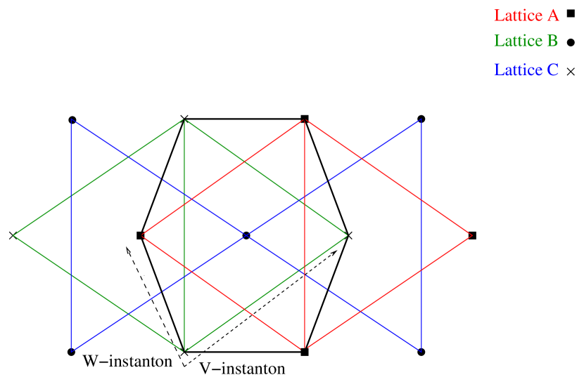
Figure 2: Points on the three triangular sublattices A, B and C: at $\gamma=(2k+1)\pi/3$, the energies of two sublattices are degenerate and the minima of the boundary potential span a honeycomb lattice, whose sites are connected by W-instanton trajectories, shorter than the V-instanton trajectories, connecting sites on the same sublattice. The black honeycomb is an elementary cell of the lattice of the minima emerging at $\gamma=\pi/3$.

$$\langle\tilde{V}^{\pm}_{j}(\tau)\tilde{V}^{\mp}_{i}(\tau^{\prime})\rangle\propto\delta_{j,i}\left[e^{\frac{\pi v\tau}{L}}-e^{\frac{\pi v\tau^{\prime}}{L}}\right]^{-\frac{8g}{3}}\>\>\>\>,$$ (25)

and, thus, the scaling dimension of $\tilde{V}^{\pm}_{j}(\tau),j=1,2,3$, is given by $h_{S}(g)=\frac{4g}{3}$. As a result, the SFP is stable for $g>3/4$ and for $\gamma\neq(2k+1)\pi/3$. Thus, for $3/4<g<1$ and for $\gamma\neq(2k+1)\pi/3$, both the WFP, and the SFP are stable and, accordingly, the phase diagram allows for a repulsive FFP. For $g>1$ and for $\gamma\neq(2k+1)\pi/3$, the SFP is the only IR stable fixed point: the set of the allowed eigenvalues of $(P_{1},P_{2})$ depends upon the value of $\gamma$, as discussed above. Accordingly, the fixed point partition function is given by ${\bf Z}_{\ell}[\vec{\mu}]$ in Eq.(22), for a pertinent choice of $\ell$. Remarkably, this shows that the SFP is time-reversal invariant, even if the “bare” value of $\gamma$ breaks this symmetry. This is not surprising, though, as the symmetry of the system at the IR stable fixed-point is usually higher than the symmetry of the microscopic system.

For $\gamma=(2k+1)\pi/3$, the sets of minima belonging to two sublattices have the same energy. As a result, the eigenvalues of the zero-mode operators lie all on a honeycomb lattice obtained by merging two triangular sublattices, as sketched in Fig.2 for $\gamma=\pi/3$, at which point the sublattices A and B merge into a honeycomb lattice. The leading perturbation near the Dirichlet fixed point contains, now, operators representing “shorter” jumps between neighboring minima on the honeycomb lattice (“W-instantons”).

Following Ref.[15], one may describe these instantons by introducing an isospin operator $\vec{\tau}$, acting on a pertinent two-component spinor . As a result, the leading boundary perturbation may now be written as

$$H_{B}=-\xi\sum_{i=1}^{3}\{\tau^{+}W_{i}^{\dagger}(\tau)+\tau^{-}W_{i}(\tau)\}\>\>\>\>,$$ (26)

with $W_{j}(\tau)=:\exp\left[\frac{2}{3}i\vec{\alpha}_{j}\cdot\vec{\psi}(\tau)\right]:$ and $\xi\sim E_{J}-E_{W}$. Since the boundary interaction contains the isospin operators $\vec{\tau}$, the relevant O.P.E.’s are obtained by combining the multiplication rules for the isospin operators

$$\tau^{z}\tau^{\pm}=\pm\tau^{\pm}\;\;\;;\;\;\tau^{\pm}\tau^{\mp}=1\pm\tau^{z}\;\;\>\>,$$ (27)

with the O.P.E.’s of the bosonic vertex operators

$$\left\{:e^{\left[\pm\frac{2}{3}i\vec{\alpha}_{j}\cdot\vec{\psi}(\tau)\right]}::e^{\left[\mp\frac{2}{3}i\vec{\alpha}_{j}\cdot\vec{\psi}(\tau^{\prime})\right]}:\right\}_{\tau^{\prime}\to\tau^{-}}\approx\left[\frac{\pi v(\tau-\tau^{\prime})}{L}\right]^{-\frac{4g}{9}}\left[1\pm\frac{2}{3}(\tau-\tau^{\prime})\vec{\alpha}_{j}\cdot\frac{\partial\vec{\psi}(\tau)}{\partial\tau}\right]\>\>\>\>.$$ (28)

Terms proportional to $\frac{\partial\vec{\psi}(\tau)}{\partial\tau}$, which could be generated to second-order in $\xi$, are suppressed by the condition $\sum_{j=1}^{3}\vec{\alpha}_{j}=0$. As a result, higher-order contributions to the $\beta$-function of the running coupling strength $\zeta=L\xi$ only appears to order $\zeta^{3}$. The RG equation for $\zeta$ is then given by

$$\frac{d\zeta}{d\ell}=[1-h_{F}(g)]\zeta-2\zeta^{3}\>\>\>\>.$$ (29)

For $\gamma=\pi/3$ the scaling dimension of the boundary interaction, $h_{F}(g)$, gets renormalized as

$$\frac{dh_{F}(g)}{d\ell}=-h_{F}(g)\zeta^{3}\>\>\>\>.$$ (30)

For a small enough value of $\zeta$, the renormalization of $h_{F}(g)$ may be safely neglected, since it appears only to the third-order in $\zeta$, and one may substitute $h_{F}(g)$ in Eq.(29) with its bare value $\frac{4g}{9}$. Thus, the leading boundary perturbation at the SFP is irrelevant for $g>9/4$, while it is relevant for $g<9/4$. As a result, for $\gamma=\frac{\pi}{3}$, there is a range of values of $g$ -namely, $1<g<9/4$- where neither the WFP, or the SFP, are stable. The flow diagram then implies the existence of a FFP in the phase diagram. In Fig.3, the phase diagram is sketched for different values of $g$: because of the periodicity in $\gamma$, only the stripe $0\leq\gamma\leq 2\pi/3$ is drawn.

The new attractive FFP emerges as a result of the combined effect of the design of the YJJN and of the possibility of tuning the frustration parameter $\gamma$ by setting the dimensionless flux $f$ to $\pi$. Since the circular array C can have a very small diameter, self-impedance effects should be negligible. For $Y$-shaped bosonic networks realized with neutral atomic systems [2], the FFP is always repulsive, since those systems are insensitive to external magnetic fluxes.

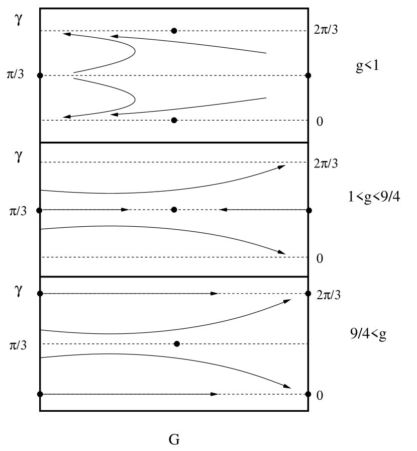
Figure 3: Phase diagram of a YJJN for (from top to bottom): $g<1$ (the only IR stable fixed point is at $G_{*}=0$); $1<g<9/4$ (the IR stable fixed point is either at $G_{*}=\infty$, or at a finite $G_{*}$, according to the initial value of $\gamma$); $9/4<g$ (the only fixed point is at $G_{*}=\infty$).

4 The Josephson currents

In this section, we probe the behavior of a YJJN near each one of its fixed points by computing the current-phase relation of the Josephson currents along the three arms of a YJJN.

We find that, for any value of $g$ and for $\gamma\neq\frac{\pi}{3}$, the current-phase relation is the same as the one of a Josephson junction chain with a weak link analyzed in Ref.[11] while, for $\gamma=\frac{\pi}{3}$, one finds new and unexpected behaviors.

The Josephson currents in the three arms of a $Y$-shaped JJN are given by

$$I_{1} = \frac{e^{*}}{\beta g}\left[\frac{1}{\sqrt{2}}\frac{\partial\ln{\bf Z}}{\partial\mu_{1}}+\frac{1}{\sqrt{6}}\frac{\partial\ln{\bf Z}}{\partial\mu_{2}}\right]$$

$$I_{2} = \frac{e^{*}}{\beta g}\left[-\frac{1}{\sqrt{2}}\frac{\partial\ln{\bf Z}}{\partial\mu_{1}}+\frac{1}{\sqrt{6}}\frac{\partial\ln{\bf Z}}{\partial\mu_{2}}\right]$$

$$I_{3} = -\sqrt{\frac{2}{3}}\frac{e^{*}}{\beta g}\frac{\partial\ln{\bf Z}}{\partial\mu_{2}}\>\>\>\>,$$ (31)

where ${\bf Z}$ is the partition function describing the thermodynamical behavior of the YJJN, $\vec{\mu}$ are the phase differences introduced in section 2.2, and $e^{*}=2e$ is the charge of a Cooper pair. In the following, we shall provide the explicit form of Eq.(31) near each one of the three accessible fixed points analyzed in section 3.

4.1 The weakly coupled fixed point

At the WFP, for $g<1$, $H_{B}$ is an irrelevant perturbation and, thus,

$${\bf Z}={\rm Tr}\biggl{\{}e^{-\beta H_{0}}{\bf T}_{\tau}\exp\left[i\int_{0}^{\beta}\>d\tau\>H_{B}(\tau)\right]\biggr{\}}\>\>\>\>,$$ (32)

may be safely computed using a mean-field approximation. In Eq.(32), $H_{0}=\frac{\pi v}{L}\sum_{j=1,2}\>\sum_{n=1}^{\infty}\alpha_{j}(-n+1)\alpha_{j}(n)$, and the boundary interaction Hamiltonian has been defined in Eq.(9). As a result, one gets

$${\bf Z}\approx{\bf Z}_{0}\exp\left[-\int_{0}^{\beta}\>d\tau\>\langle H_{B}(\tau)\rangle_{0}^{(W)}\right]={\bf Z}_{0}\exp\left[2\beta\bar{E}_{W}\sum_{i=1}^{3}\cos[\vec{\alpha}_{i}\cdot\vec{\mu}+\gamma]\right]\>\>\>\>,$$ (33)

where $\langle\ldots\rangle_{0}$ denotes the thermal average with Boltzmann weight $e^{-\beta H_{0}}$, and ${\bf Z}_{0}={\rm Tr}[e^{-\beta H_{0}}]=1/\{\prod_{n=0}^{\infty}[1-\bar{q}^{n+\frac{1}{2}}]^{2}\}$. From Eqs.(31,33), one gets

$$I_{1} = \frac{2e^{*}\bar{E}_{W}}{g}\{\sin[\vec{\alpha}_{1}\cdot\vec{\mu}+\gamma]-\sin[\vec{\alpha}_{3}\cdot\vec{\mu}+\gamma]\}$$

$$I_{2} = \frac{2e^{*}\bar{E}_{W}}{g}\{\sin[\vec{\alpha}_{2}\cdot\vec{\mu}+\gamma]-\sin[\vec{\alpha}_{1}\cdot\vec{\mu}+\gamma]\}$$

$$I_{3} = \frac{2e^{*}\bar{E}_{W}}{g}\{\sin[\vec{\alpha}_{3}\cdot\vec{\mu}+\gamma]-\sin[\vec{\alpha}_{2}\cdot\vec{\mu}+\gamma]\}\>\>\>\>.$$ (34)

Eqs.(34) explicitly show the dependence of the current’s patterns along the arms of the YJJN on both the phase differences $\vec{\mu}$ and the parameter $\gamma$.

4.2 The strongly coupled fixed point

In order to compute the Josephson currents across the three arms of a YJJN at the SFP, one has now to account for the contribution coming from the zero modes. In order to do so, one should use Eqs.(31), with the appropriate expression for the partition function ${\bf Z}_{\ell}[\vec{\mu}]$ given by Eq.(22). The zero modes affect the total energy by the amount

$$E_{n_{12},n_{13}}[\vec{\mu}]=\frac{\pi vg}{L}\left[\left(n_{12}+\frac{\mu_{1}}{2\pi}+\frac{2\epsilon_{\ell}}{3}\right)^{2}+\frac{4}{3}\left(n_{13}+\frac{n_{12}}{2}+\frac{\sqrt{3}}{4\pi}\mu_{2}\right)^{2}\right]\>\>\>\>,$$ (35)

which is a function of $n_{12},n_{13},\vec{\mu}$. At very low temperature and at fixed $\vec{\mu}$, one may approximate the free energy ($-\frac{1}{\beta}\ln{\bf Z}$) with the lowest value of the energies $E_{n_{12},n_{13}}[\vec{\mu}]$, given in Eq.(35). For the zero mode eigenvalues belonging to sublattice A, for instance, the Josephson currents turn out to be given by

$$I_{1} = \frac{e^{*}vg}{L}\left[\frac{1}{\sqrt{2}}\left(\frac{\mu_{1}}{2\pi}+n_{12}\right)+\frac{1}{\sqrt{6}}\left(\frac{\mu_{2}}{2\pi}+\frac{2n_{13}+n_{12}}{\sqrt{3}}\right)\right]$$

$$I_{2} = \frac{e^{*}vg}{L}\left[-\frac{1}{\sqrt{2}}\left(\frac{\mu_{1}}{2\pi}+n_{12}\right)+\frac{1}{\sqrt{6}}\left(\frac{\mu_{2}}{2\pi}+\frac{2n_{13}+n_{12}}{\sqrt{3}}\right)\right]$$

$$I_{3} = -\frac{e^{*}vg}{L}\sqrt{\frac{2}{3}}\left(\frac{\mu_{2}}{2\pi}+\frac{2n_{13}+n_{12}}{\sqrt{3}}\right)\>\>\>\>.$$ (36)

Eqs.(36) show the usual [11] sawtooth dependence on the phase difference $\vec{\mu}$, exhibited by the Josephson current at the SFP. As $\vec{\mu}$ varies within one periodicity interval, the integers $n_{12},n_{13}$ change by $\pm 1$. For instance, for $-\frac{1}{6}<\frac{\mu_{1}}{2\pi}<\frac{1}{6}$, from $\frac{\mu_{2}}{2\pi}=\frac{\mu_{2}^{*}}{2\pi}-\delta=-\frac{1}{\sqrt{3}}-\delta$ to $\frac{\mu_{2}}{2\pi}=\frac{\mu_{2}^{*}}{2\pi}+\delta$ ($\delta/\pi\ll 1$), the Josephson currents undergo an abrupt jump from

$$I_{1}=\frac{e^{*}v}{\sqrt{2}(2\pi)L}\left(\frac{\mu_{1}}{2\pi}-\frac{1}{3}\right)\>\>\>,\>\>I_{2}=\frac{e^{*}v}{\sqrt{2}(2\pi)L}\left(-\frac{\mu_{1}}{2\pi}-\frac{1}{3}\right)\;\;\;,\;\;I_{3}=\frac{\sqrt{2}e^{*}v}{6\pi L}\>\>\>\>,$$ (37)

to

$$I_{1}=\frac{e^{*}v}{\sqrt{2}(2\pi)L}\left(\frac{\mu_{1}}{2\pi}+\frac{1}{3}\right)\>\>\>,\>\>I_{2}=\frac{e^{*}v}{\sqrt{2}(2\pi)L}\left(-\frac{\mu_{1}}{2\pi}+\frac{1}{3}\right)\;\;\;,\;\;I_{3}=-\frac{\sqrt{2}e^{*}v}{6\pi L}\>\>\>\>,$$ (38)

corresponding to the shift $(n_{12},n_{13})\longrightarrow(n_{12},n_{13}+1)$.

It should be noticed that, for $\frac{\mu_{1}}{2\pi}=-\frac{1}{3}$, the current in arm 1 switches from 0 to a finite value, while the current in arm 2 does the opposite. This suggests that a YJJN may be useful as a switch commuting between two states macroscopically distinguishable by the value of the Josephson current across the circuit branches. Finally we mention that, as it usually happens in superconducting networks [12, 14], the V-instantons near the Dirichlet fixed point round off the spikes of the sawtooth function describing the Josephson current phase relationship. This effect is discussed in detail in appendix B.

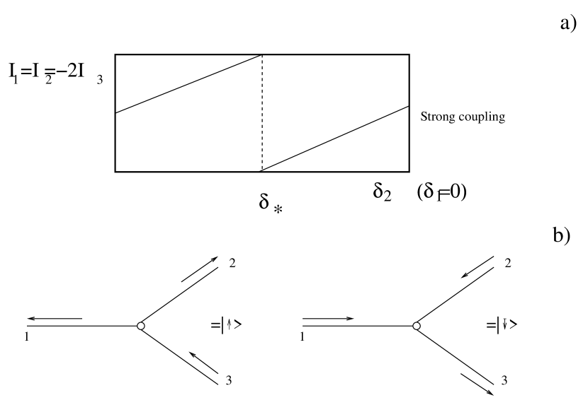
Figure 4: a): Behavior of the Josephson current across the three chains near the SFP, with the phases $\mu_{1},\mu_{2}$ chosen as in section 4.2. b): Sketch of the Josephson current pattern in the YJJN corresponding to the current patterns across $\mu_{2}=\mu_{2}^{*}$.

4.3 Instanton effects for $\gamma=\pi/3$ at the finite coupling fixed point

For $\gamma=\pi/3$, near the FFP, new more dramatic instanton effects take place in a YJJN. Indeed, for $\gamma=\pi/3$, two triangular sublattices become degenerate and shorter instanton paths are allowed. As evidenced in section 3, the operators $W_{j},W_{j}^{\dagger}$ representing these paths, become relevant for $1<g<\frac{9}{4}$, and drive the system away from the Dirichlet point. Here we evidence the remarkable effects of W-instantons on the distribution of the Josephson currents in the arms of a YJJN.

For $\gamma=\frac{\pi}{3}$, the minima of the boundary interaction lie on the honeycomb lattice depicted in Fig.2. Their position is given by

$$(p_{1},p_{2})=\sqrt{2g}\left(\left[n_{12}+\frac{\mu_{1}}{2\pi}+\frac{2\epsilon}{3}\right],\left[\frac{\mu_{2}}{2\pi}+\frac{2}{\sqrt{3}}\left(n_{13}+\frac{n_{12}}{2}\right)\right]\right)\>\>\>\>,$$ (39)

with $\epsilon=0,1$. Setting $\mu_{1}\sim\mu_{1}^{*}+\delta=-\frac{\pi}{3}-\delta$, and $-\frac{\pi}{\sqrt{3}}<\mu_{2}<\frac{\pi}{\sqrt{3}}$, with $|\delta|/\pi\ll 1$, the state $|\uparrow\rangle=|0,0\rangle_{A}$ and the state $|\downarrow\rangle=|0,0\rangle_{B}$ are quasidegenerate (indeed, they become exactly degenerate for $\delta=0$). For this choice of the quasidegenerate states, the W-instantons are described by $W(0)=-2\zeta:\cos\left[\frac{2}{3}\psi_{1}(0)\right]:$. Substituting Eq.(66) into Eq.(67) allows to write their contribution to the partition function as

$${\bf Z}[\delta,\mu_{2}] = \sum_{\sigma}\int_{-\infty}^{\infty}\>dx\>\frac{e^{i\frac{g\pi v\beta}{2L}x}}{2\pi}\biggl{\{}ix+e_{0}+{\rm sg}(\sigma)\alpha\delta-\zeta^{2}\Gamma[1-2h_{F}(g)][ix+e_{0}+{\rm sg}(\sigma)\alpha\delta]^{2h_{F}(g)-1}\biggr{\}}\biggl{/}$$ (40)

$$\biggl{\{}[ix+e_{0}]^{2}-[\alpha^{2}\delta^{2}+\zeta^{2}]-\zeta^{2}\Gamma[1-2h_{F}(g)]\sum_{\gamma}[ix+e_{0}+{\rm sg}(\gamma)\alpha\delta]^{2h_{F}(g)}$$

$$- \zeta^{4}\Gamma^{2}[1-2h_{F}(g)][(ix+e_{0})^{2}-\alpha^{2}\delta^{2}]^{2h_{F}(g)-1}\biggr{\}}\>\>\>\>,$$

where $\alpha=g/(6\pi)$, $e_{0}\equiv e_{0}(\delta,\mu_{2})=g\left(\frac{1}{9}+\frac{\delta^{2}}{4\pi^{2}}+\frac{\mu_{2}^{2}}{4\pi^{2}}\right)$, $x=\frac{2L}{\pi v}\omega$, and ${\rm sg}(\sigma)=1$ if $\sigma=\uparrow$, $=-1$, if $\sigma=\downarrow$.

To compute Eq.(40) is quite a formidable task: however, an approximate computation can be carried out, for $g=\frac{9}{4}-\epsilon$ ($\epsilon\ll 1$), near the FFP $\zeta_{*}=(1-\frac{4g}{9})^{\frac{1}{2}}$. Indeed, since = $\zeta_{*}\sim\epsilon^{\frac{1}{2}}\ll 1$, neglecting $O(\zeta_{*}^{4})$-terms in Eq.(40), leads to

$${\bf Z}[\delta,\mu_{2}]\approx\exp\left[-\beta\frac{\pi v}{L}e_{0}(\delta,\mu_{2})\right]\left\{\cosh\left[\beta\frac{\pi v\alpha}{L}\delta\right]+\cosh\left[\beta\frac{\pi v\alpha}{L}\sqrt{\alpha^{2}\delta^{2}+3\zeta_{*}^{2}}\right]\right\}\>\>\>\>,$$ (41)

from which, for $\beta v/L\gg 1$, one gets

$$I_{1} \approx \frac{e^{*}v}{2\pi L}\left\{\frac{\delta}{\sqrt{2}}\left[-1+\frac{4\pi^{2}\alpha^{2}}{\sqrt{\alpha^{2}\delta^{2}+3\zeta_{*}^{2}}}\right]-\frac{\mu_{2}}{\sqrt{6}}\right\}$$

$$I_{2} \approx \frac{e^{*}v}{2\pi L}\left\{-\frac{\delta}{\sqrt{2}}\left[-1+\frac{4\pi^{2}\alpha^{2}}{\sqrt{\alpha^{2}\delta^{2}+3\zeta_{*}^{2}}}\right]-\frac{\mu_{2}}{\sqrt{6}}\right\}$$

$$I_{3} \approx \frac{e^{*}v}{2\pi L}\sqrt{\frac{2}{3}}\mu_{2}\>\>\>\>.$$ (42)

Eqs.(42) yield the current-phase relations near the attractive FFP shown in Fig.5. The typical sawtooth behavior of the Josephson current-phase relation is now associated to a stable attractive FFP in the phase diagram.

Usually, in superconducting systems, such as SQUIDs [14, 12] and Josephson chains with localized impurities [13, 11], either the smoothening of the spikes of the sawtooth function describing the Josephson current-phase relationship at strong coupling is a perturbative effect, or the SFP is unstable, since quantum fluctuations drive the system to the WFP. At variance, for a YJJN at the FFP, the smoothening of the spikes of the Josephson current due (now) to the W-instantons is a nonperturbative effect and the FFP is a stable attractive fixed point in the phase diagram. Since a sawtooth behavior of the Josephson current is usually associated [14, 11, 12] to the emergence of a macroscopically quantum coherent two-level system in the superconducting device [17], one may safely expect that an effective macroscopic two-level quantum system -this time robust against quantum fluctuations- may emerge in a YJJN, as well. This issue has been addressed in Ref.[21] and will be revisited in the next section.

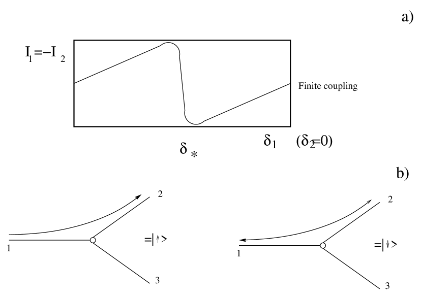
Figure 5: a): Behavior of the Josephson current across the chains 1 and 2 near the FFP, with the phases $\mu_{1},\mu_{2}$ chosen as discussed in section 4.3. b): Sketch of the Josephson current pattern in the YJJN associated to the macroscopic states $|\sigma(=\uparrow,\downarrow)\rangle$ introduced in section 4.3.

5 A quantum two-level system emerging in a YJJN

In this section, we revisit the arguments given in Ref.[21] to show that an effective quantum two-level system with frustrated decoherence [22] may emerge from a YJJN near the FFP.

As evidenced in appendix A, the energy of the long-wavelength excitations of the YJJN is given by

$$E=\frac{\pi v}{2L}[\vec{p}]^{2}+E^{\prime}\;\;\;\;,$$ (43)

where $\vec{p}=(p_{1},p_{2})$ is the eigenvalue of the zero-mode operators $\vec{P}=(P_{1},P_{2})$, introduced in section 3, and $E^{\prime}$ accounts for the energy of the plasmon modes described by the TLL Hamiltonian given by Eq.(7). Plugging Eqs.(19,20) into Eq.(43) yields the explicit dependence of the energy on the minima on the phases $\varphi_{j}$ of the three bulk superconductors.

It is easy to see that, for any value of $\gamma$ and for all possible values of the Luttinger parameter $g$, it is always possible, for a finite YJJN, to choose the phase differences $\mu_{1}$ and $\mu_{2}$ to obtain two low-energy quasidegenerate states, well separated from the rest of the spectrum. Slightly generalizing the notation introduced in Section 4, we still denote the two quasidegenerate states by $|\uparrow\rangle$ and $|\downarrow\rangle$ and observe that, for $\gamma\neq(2k+1)\pi/3$, both states belong to the same triangular sublattice (A, B or C), while, for $\gamma=(2k+1)\pi/3$, they belong - as in Section 4- to two different sublattices.

The dynamics of the two states $|\uparrow\rangle$ and $|\downarrow\rangle$ interacting with the plasmon modes residing on the three chains of the Y-junction may be written as

$$H_{2}=[E_{\uparrow}(\vec{\mu})-E_{\downarrow}(\vec{\mu})]\sigma^{z}-Y{\bf O}(0)\sigma^{-}-Y{\bf O}^{\dagger}(0)\sigma^{+}\>\>\>\>,$$ (44)

where ${\bf O}$ is one of the vertex operators $V_{j}$ (if the states lie on the same triangular sublattice), or $W_{j}$ (if the states lie on the honeycomb lattice obtained by merging two triangular sublattices), and $\sigma^{z}=\sum_{\sigma=\uparrow,\downarrow}\frac{1}{2}{\rm sg}(\sigma)|\sigma\rangle\langle\sigma|$, $\sigma^{+}=|\uparrow\rangle\langle\downarrow|$, $\sigma^{-}=|\downarrow\rangle\langle\uparrow|$. In Eq.(44), $E_{\uparrow}(\vec{\mu})$ and $E_{\downarrow}(\vec{\mu})$ are the energies associated to the states $|\uparrow\rangle$ and $|\downarrow\rangle$, respectively. The $\sigma^{z}$-term contributes only if the $|\uparrow\rangle$ and the $|\downarrow\rangle$ states are quasidegenerate, which may be achieved by a slight detuning of the phase differences $\mu_{1}$ and $\mu_{2}$ by an amount $\delta$ ($\ll 2\pi$). The terms proportional to $Y$ describe an effective field in the $x$-direction and, at the same time, the coupling between the transverse components of the spin and the bath provided by the plasmon modes of the three chains: on one hand they determine a $Y$-dependent renormalization of the energies of the effective two-level system -the tunnel splitting of the energies of the states $|\sigma\rangle$-, on the other hand, they may lead to the formation of an entangled state between the two-level system and the bath formed by the plasmon modes in the network. This latter effect is a main source of decoherence in a two-level system interacting with one (or more) baths [22, 21].

Depending on whether $\gamma\neq(2k+1)\pi/3$, or $\gamma=(2k+1)\pi/3$ and on the value of the Luttinger parameter $g$ the interaction of the system with the bath provided by the plasmon modes of the network leads to different coherent behaviors of the YJJN [21]. In the following we shall compute the spectral density of the two level system near the SFP and the FFP; as pointed out in Ref.[22], the spectral density provides a measure of the amount of entanglement between a two level system and the pertinent environmental modes.

5.1 Spectral density of the two-level system near the strongly-coupled fixed point

As evidenced in section 3, for $1<g<9/4$ and $\gamma\neq(2k+1)\pi/3$, or for $g>9/4$ and $\forall\gamma$, the YJJN exhibits an IR stable SFP in its phase diagram. If $-\pi/3<\gamma<\pi/3$, Eq.(19) implies that the quasidegenerate states $|\uparrow\rangle$ and $|\downarrow\rangle$ lie on the triangular sublattice A and that Eq.(44) may be explicitly written as

$$H_{2,{\rm SFP}}=[E_{\uparrow}(\vec{\mu})-E_{\downarrow}(\vec{\mu})]\sigma^{z}-YV(0)\sigma^{-}-YV^{\dagger}(0)\sigma^{+}\>\>\>\>,$$ (45)

where $V(0)$ is the V-instanton vertex operator.

To compute the spectral density of the two-level system in Eq.(45) one needs to evaluate $\chi^{``}_{\perp}(\Omega)/\Omega$ vs. $\Omega$, where $\chi^{``}_{\perp}(\Omega)$ is the imaginary part of the transverse dynamical spin susceptibility. Since V-instantons are an irrelevant perturbation, by neglecting higher-order corrections in $Y$ (see appendix B), one gets

$$\frac{\chi^{``}_{\perp}(\Omega)}{\Omega}\propto\delta(\Omega-2\Delta(\vec{\mu}))+\delta(\Omega+2\Delta(\vec{\beta}))\>\>\>\>,$$ (46)

with $\Delta(\vec{\mu})=\sqrt{[E_{\uparrow}(\vec{\mu})]^{2}+Y^{2}}$. From Eq.(46) one sees that the spectrum of Eq.(45) is given by two classical states, with $\Omega=\pm\Delta(\vec{\mu})$. As pointed out in ref. [21] this behavior signals that there is no entanglement between the two level quantum system and the plasmon modes. Since $Y$ is irrelevant (i.e., its fixed point value is $Y_{*}=0$), there is not even tunnel splitting between the two degenerate states, no quantum coherence may emerge in this regime [21]

5.2 Spectral density of the two-level system near the finite-coupling fixed point

For $1<g<9/4$ and $\gamma=\pi/3$, the two states $|\uparrow\rangle$ and $|\downarrow\rangle$ lie on nearest neighboring sites on the honeycomb lattice obtained by merging the sublattices A and B. As evidenced in section 3, short W-instantons are a relevant perturbation at the SFP and render the FFP IR stable. Near the FFP, the two-level system is described by

$$H_{2,{\rm FFP}}=[E_{\uparrow}(\vec{\mu})-E_{\downarrow}(\vec{\mu})]\sigma^{z}-\xi W(0)\sigma^{-}-\xi W^{\dagger}(0)\sigma^{+}\>\>\>\>,$$ (47)

where, now, $W(0)$ is a W-instanton operator. The computation of the spectral density $\chi_{\perp}^{``}(\Omega)$ is detailed in appendix B using a self-consistent RPA approximation. As a result, the spectral density has now two peaks centered at $\pm\Delta_{*}(\vec{\mu})=\pm\sqrt{[E_{\uparrow}(\vec{\mu})]^{2}+(\zeta_{*}/L)^{2}}$, with a finite width $\propto\frac{\pi v}{L}(\zeta_{*})^{1+\frac{8}{9}g}$, where $\zeta_{*}$ is the finite fixed point value of the running coupling constant, determined in section 3. The spectral density is plotted in Fig.6, where we report, for completeness, also the spectral density arising near the WFP [21].

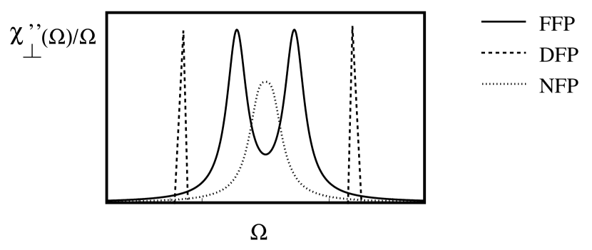
Figure 6: Behavior of the spectral density $\chi^{``}_{\perp}(\Omega)/\Omega$ vs. $\Omega$ near the WFP, the SFP, and the FFP.

6 Concluding remarks

We showed that, for $1<g<9/4$ and for $f=\pi$, an attractive FFP emerges in the phase diagram accessible to a YJJN. The new fixed point does not break time-reversal invariance, and it is a stable, attractive fixed point only when the dimensionless flux threading the cental loop equals $\pi$; for $f\neq\pi$, we have shown that only the SFP survives as a stable attractive fixed point. Our results show remarkable similarities between the phase diagram accessible to a YJJN and the one arising in the analysis of the quantum Brownian motion on a frustrated triangular lattice [15, 16].

Crucial to our analysis is the fact that, at $f=\pi$ - for $1<g<9/4$ - the W-instantons become a relevant perturbation and, thus, destabilize the SFP. These instantons emerge ultimately as a result of the Y-shaped geometry of the network, since they arise when the minima of the boundary potential span the honeycomb lattice depicted in Fig.2. Intuitively, they may be regarded as the result of the “deconfinement” of the V-instantons in its elementary constituents happening- when $1<g<9/4$- only at $f=\pi$. A Coulomb gas approach could be a very helpful tool to further clarify the nature of the FFP.

We computed the current-phase relations along the arms of the YJJN near each one of the allowed fixed points. We evidenced the parameter regions where a YJJN may be operated as a Josephson switch and we showed the different effects of the instantons on the current pattern near the SFP and the FFP. In particular, in a YJJN at the FFP, the smoothening of the spikes of the sawtooth dependence of Josephson current on the phase differences $\vec{\mu}$ is a nonperturbative effect, due to the attractive nature of this fixed point.

Finally, we provided additional arguments confirming that, near the FFP, a YJJN supports a quantum coherent two-level system with frustrated decoherence [21].

In order to set a YJJN to be a quantum device either acting as a Josephson current switch or modeling an effective two level quantum system one needs, first of all, to promote the phase differences $\mu_{1},\mu_{2}$ to control parameters. This may be achieved by resorting, for instance, to multipolar magnetic coils [23] inserted in external loops connecting the bulk superconductors at the outer boundary of the YJJN: indeed, for sufficiently long chains, the localized magnetic fields generated by the multipolar magnetic coil may be engineered to avoid variations in the flux threading the circular Josephson junction array C. Furthermore, when the YJJN has a finite size $L$, it is easy to convince oneself that the FFP is stable against small fluctuations of the flux $f$, provided that $v/L$ is sufficiently big: for instance, if the point $\gamma=\pi/3$ is displaced by a small amount $\nu$, $v/L$ needs to be larger than the energy splitting $\bar{E}_{W}\sin(\nu)$ between the minima of two triangular sublattices. At variance, when $v/L<\bar{E}_{W}\sin(\nu)$, there is a flow towards the SFP and, depending on ${\rm sgn}(\nu)$, the minima of the boundary potential lie on either one of the triangular A and B sublattices [21]. Finally, today ’s technology allows to fabricate superconducting devices with values of $g$ ranging from $g<1$, to $g\sim 2$ [24].

Josephson networks where $n$ finite chains are connected to a central circular array ${\bf C}$ may be analyzed with tools similar to those used in this paper. Of interest is also the JJ network with $n=4$ since it corresponds to the tetrahedral qubit proposed in Ref.[25].

Acknowledgments : We thank I. Affleck, C. Chamon, R. Russo and A. Trombettoni for fruitful discussions and correspondence. We thank the Particle Theory Sector of S.I.S.S.A. - I.S.A.S. and the High Energy Theory Group of I.C.T.P. for hospitality during the final stages of our work.

Appendix A Tomonaga-Luttinger description of superconducting Josephson junction arrays

Here, we briefly review the derivation of the effective TLL Hamiltonian, describing one-dimensional arrays of Josephson junctions. For this purpose, in Eq.(6) one should assume that $E_{J}/E_{c}\ll 1$ and ${\bf N}=2n+1+2h$, with $n$ integer and $|h|\ll 1$ [13, 11]; then, if one defines effective lattice spin-1/2 operators as

$$S_{j}^{z}={\bf P}_{G}\left[-i\frac{\partial}{\partial\phi_{j}}-\frac{{\bf N}}{2}\right]{\bf P}_{G}\;\;\;,\;\;S_{j}^{\pm}={\bf P}_{G}e^{\pm i\phi_{j}}{\bf P}_{G}\;\;\;\;,$$ (48)

with ${\bf P}_{G}$ the operator projecting onto the subspace of the charge eigenstates with the charge at any site either equal to $n$ or to $n+1$, one may present Eq.(6) as

$$P_{\bf G}^{\dagger}H_{\rm chain}P_{\bf G}\equiv H_{\rm spin}=-\frac{E_{J}}{2}\sum_{j=1}^{L/a-1}[S_{j}^{+}S_{j+1}^{-}+S_{j+1}^{+}S_{j}^{-}]$$

$$+\left[E_{z}-\frac{3}{16}\frac{(E_{J})^{2}}{E_{c}}\right]\sum_{j=1}^{L/a-1}S_{j}^{z}S_{j+1}^{z}-H\sum_{j=1}^{L/a}S_{j}^{z}\>\>\>\>.$$ (49)

Eq.(49) is the Hamiltonian for an XXZ-chain in an external magnetic field $H=hE_{c}$ [13, 11]: to map it onto an effective TLL Hamiltonian, one needs to write the spin operators in terms of lattice Jordan-Wigner fermions $a_{j}$. Upon defining the lattice Fourier modes $a_{k}$ as

$$a_{k}=\sqrt{\frac{a}{L}}\sum_{j=1}^{L/a}a_{j}e^{-ik(ja)}\>\>\>;\>\>(k=\frac{2\pi n}{L}\>,\;n=1,\ldots,L/a)\>\>\>\>,$$ (50)

$P_{\bf G}^{\dagger}H_{\rm chain}P_{\bf G}$ in Eq.(49) is given by

$$H_{\rm JW}=\sum_{k}[-E_{J}\cos(ka)-H]a^{\dagger}_{k}a_{k}+\left[E_{z}-\frac{3}{16}\frac{(E_{J})^{2}}{E_{c}}\right]\sum_{j=1}^{L/a-1}(a_{j}^{\dagger}a_{j}-\frac{1}{2})(a_{j+1}^{\dagger}a_{j+1}-\frac{1}{2})\>\>\>\>.$$ (51)

From Eq.(51), one see that two ”band-insulating” phases open up when $|H|\geq E_{J}$ [13, 11]. In spin coordinates, they correspond to fully polarized spin phases which are the Coulomb blockade insulating phases setting in the chain when the gate voltage is tuned far from charge degeneracy point.

For $|H|<E_{J}$, Eq.(51) describes a one-dimensional conductor. By keeping only long-wavelength modes around the Fermi points $k_{f}^{\pm}=\pm\frac{1}{a}{\rm arccos}(H/E_{J})$, and by bosonizing Eq.(51) one gets the Sine-Gordon Hamiltonian

$$H^{b}=\frac{g}{4\pi}\>\int_{0}^{L}\>dx\>\left[\frac{1}{v}\left(\frac{\partial\Phi}{\partial t}\right)^{2}+v\left(\frac{\partial\Phi}{\partial x}\right)^{2}\right]-G_{U}\>\int_{0}^{L}\>dx\>\cos[2\sqrt{2}g\Phi(x)+4k_{f}x]\>\>\>\>,$$ (52)

with the Luttinger parameter defined in section 2 and $G_{U}\propto\left[E^{z}-\frac{3}{16}\frac{(E_{J})^{2}}{E_{c}}\right]$. When $g>1/2$, the last term in Eq.(52) may be neglected, in the thermodynamic limit and $H^{b}$ reduces to the Hamiltonian of a spinless TLL. $g$ may either be $<1$, or $>1$, depending on whether $\Delta(=\left[E^{z}-\frac{3}{16}\frac{(E_{J})^{2}}{E_{c}}\right])>0$ (repulsive TLL), or $\Delta<0$ (attractive TLL) [11].

The normal modes of a spinless TLL may be constructed by introducing the dual field $\psi$, related to $\Phi$ by $\frac{1}{v}\frac{\partial\psi}{\partial t}=\frac{\partial\Phi}{\partial x}$ and $\frac{1}{v}\frac{\partial\Phi}{\partial t}=\frac{\partial\psi}{\partial x}$, and by introducing two chiral bosonic fields, $\phi_{R},\phi_{L}$, as

$$\phi_{R}(x)=\sqrt{\frac{g}{2}}\Phi(x)+\frac{1}{\sqrt{2g}}\psi(x)\;\;\;;\;\;\phi_{L}(x)=\sqrt{\frac{g}{2}}\Phi(x)-\frac{1}{\sqrt{2g}}\psi(x)\;\;\;\;.$$ (53)

In terms of $\phi_{R},\phi_{L}$, $H^{b}$ is given by

$$H^{b}=\frac{v}{4\pi}\>\int_{0}^{L}\>dx\>\left[\left(\frac{\partial\phi_{R}}{\partial x}\right)^{2}+\left(\frac{\partial\phi_{L}}{\partial x}\right)^{2}\right]\>\>\>\>.$$ (54)

The normal mode expansion of $\phi_{R}(x-vt),\phi_{L}(x+vt)$ may be written in terms of the Fubini-Veneziano chiral fields [26] as

$$\phi_{R}(x-vt)=q_{R}-\frac{2\pi}{L}P_{R}(x-vt)+i\sum_{n\neq 0}\frac{\alpha_{R}(n)}{n}e^{ik_{n}(x-vt)}$$

$$\phi_{L}(x+vt)=q_{R}+\frac{2\pi}{L}P_{L}(x+vt)+i\sum_{n\neq 0}\frac{\alpha_{L}(n)}{n}e^{ik_{n}(x+vt)}\>\>\>\>,$$ (55)

with

$$[q_{R},P_{R}]=[q_{L},P_{L}]=i\;\;\;;\;\;[\alpha_{R}(n),\alpha_{R}(m)]=-[\alpha_{L}(n),\alpha_{L}(m)]=n\delta_{n+m,0}\;\;\;\;,$$ (56)

with all the other commutators vanishing. As a result:

$$H^{b}=\frac{\pi v}{L}[(P_{R})^{2}+(P_{L})^{2}]+\frac{\pi v}{L}\sum_{n\neq 0}[\alpha_{R}(-n)\alpha_{R}(n)+\alpha_{L}(n)\alpha_{L}(-n)]\>\>\>\>.$$ (57)

To construct the Fock space, one needs to define a vacuum $|(p_{R},p_{L}),0\rangle$ for any allowed pair of eigenvalues of the zero-mode operators $P_{R},P_{L}$, and then act with creation operators $\alpha_{R}(n),\alpha_{L}(-n)$ ($n<0$) on the states $|(p_{R},p_{L}),0\rangle$, which obey the conditions

$$P_{R}|(p_{R},p_{L}),0\rangle=p_{R}|(p_{R},p_{L}),0\rangle\;\;\;,\;\;P_{L}|(p_{R},p_{L}),0\rangle=p_{L}|(p_{R},p_{L}),0\rangle\>\>\>\;,$$

$$\alpha_{R}(n)|(p_{R},p_{L}),0\rangle=\alpha_{L}(-n)|(p_{R},p_{L}),0\rangle=0\;\;\;(n>0)\;\;\;\;,$$ (58)

In a system with boundaries, the boundaries conditions may be accounted for by means of pertinent relations between the _R and the _L modes. For instance, Neumann boundary conditions at $x=0$, that is, $\frac{\partial\Phi(0)}{\partial x}=0$, imply

$$P_{R}-P_{L}=0\;\;\;,\;\;\alpha_{R}(n)+\alpha_{L}(-n)=0\;\;,\;\forall n\;\;\;\;,$$ (59)

while Dirichlet boundary conditions at $x=0$, that is, $\Phi(0)=0$, imply

$$P_{R}+P_{L}=0\;\;\;,\;\;\alpha_{R}(n)-\alpha_{L}(-n)=0\;\;,\;\forall n\;\;\;\;.$$ (60)

Appendix B The partition function and the spectral density of the effective two-state system

Here we set up the general formalism needed to include the instanton contributions to the partition function of the effective two-level system described in section 5. In doing so, it is most convenient to write the spin-1/2 operators introduced in Eq.(44) by means of two pairs of fermionic operators, $a_{\sigma},a^{\dagger}_{\sigma}$, such that $\sigma^{z}=\frac{1}{2}\sum_{\sigma=\uparrow\downarrow}{\rm sg}(\sigma)a_{\sigma}^{\dagger}a_{\sigma}$, $\sigma^{+}=a_{\uparrow}^{\dagger}a_{\downarrow}$. When doing so, the imaginary time action of the effective two-level system reads as

$$S_{E}=\int_{0}^{\beta}\>d\tau\>\left\{\sum_{\sigma}\>a_{\sigma}^{\dagger}\left[\frac{\partial}{\partial\tau}-i\omega_{0}-E_{\sigma}(\vec{\mu})\right]a_{\sigma}+[a_{\uparrow}^{\dagger}a_{\downarrow}{\bf O}(\tau)+{\rm h.c.}]\right\}+S_{E}^{(0)}\>\>\>\>,$$ (61)

where $S_{E}^{(0)}$ is the Euclidean action for the plasmon field, given by

$$S_{E}^{(0)}=\sum_{j=1,2,3}\frac{g}{4\pi}\>\int_{0}^{\beta}\>d\tau\>\>\int_{0}^{L}\>dx\>\left[\frac{1}{v}\left(\frac{\partial\Phi_{j}}{\partial\tau}\right)^{2}+v\left(\frac{\partial\Phi_{j}}{\partial x}\right)^{2}\right]\;\;\;\;,$$ (62)

while the chemical potential is $i\omega_{0}=i\frac{\pi}{\beta}$ [22].

At low temperature ($\beta\frac{v}{L}\gg 1$), one may approximate the partition function of the effective two-level system as

$${\bf Z}_{\rm Eff}\approx\sum_{\sigma}{\bf Z}_{\sigma\sigma}(\beta)\;\;\;\;,$$ (63)

with ${\bf Z}_{\sigma\sigma^{\prime}}(\tau)=\langle a_{\sigma}(\tau)a_{\sigma^{\prime}}^{\dagger}(0)\rangle$.

The diagrams used to compute ${\bf Z}_{\sigma\sigma^{\prime}}(\omega)=\int_{0}^{\infty}\>d\tau\>e^{-i\omega\tau}{\bf Z}_{\sigma\sigma^{\prime}}(\tau)$ are schematically depicted in Fig.7; there, the solid thin line corresponds to the propagator of a fermion $a_{\sigma}$, given by $g^{(0)}_{\sigma}(\omega)=1/[i(\omega-\omega_{0})+E_{\sigma}(\vec{\mu})]$, and the dashed line corresponds to the propagator for the $Y$-vertex. The pertinent Dyson’s equations yielding ${\bf Z}_{\sigma\sigma^{\prime}}(\omega)$ are given by

$${\bf Z}_{\sigma\sigma}(\omega) = g_{\sigma}^{(0)}(\omega)\left\{1+Y{\bf Z}_{\bar{\sigma}\sigma}(\omega)+Y^{2}\gamma_{\bar{\sigma}}(\omega){\bf Z}_{\sigma\sigma}(\omega)\right\}$$

$${\bf Z}_{\bar{\sigma}\sigma}(\omega) = g_{\bar{\sigma}}^{(0)}(\omega)\left\{Y{\bf Z}_{\sigma\sigma}(\omega)+Y^{2}\gamma_{\sigma}(\omega){\bf Z}_{\bar{\sigma}\sigma}(\omega)\right\}\;\;\;\;,$$ (64)

where $\bar{\sigma}$ is $\uparrow(\downarrow)$ if $\sigma$ is $\downarrow(\uparrow)$, $\gamma_{\sigma}(\omega)$ corresponds to the “bubble” diagram in Fig.7 given by

$$\gamma_{\sigma}(\omega)=\int_{0}^{\infty}\>d\tau\>\theta(\tau)\>e^{-i\omega\tau}\>\gamma_{\sigma}(\tau)$$

$$=\frac{2L}{\pi v}\>\left[\frac{\Gamma[1-2h(g)]}{\frac{2L}{\pi v}(i(\omega-\omega_{0})+E_{\sigma}(\vec{\mu}))-h(g)}\right]\left[\frac{\Gamma[\frac{2L}{\pi v}(i(\omega-\omega_{0})+E_{\sigma}(\vec{\mu}))+h(g)]}{\Gamma[\frac{2L}{\pi v}(i(\omega-\omega_{0})+E_{\sigma}(\vec{\mu})-h(g)]}\right]\>\>\>\>,$$ (65)

with $h(g)=h_{S}(g)=\frac{4}{3}g$ for V-instantons, while $h(g)=h_{F}(g)=\frac{9}{4}g$ for W-instantons. When $L\omega/v\gg 1$, Eq.(65) may be approximated as

$$\gamma_{\sigma}(\omega)\approx\left(\frac{2L}{\pi v}\right)^{2h(g)}\>\Gamma[1-2h(g)]\>[i(\omega-\omega_{0})+E_{\sigma}(\vec{\mu})]^{2h(g)-1}\>\>\>\>.$$ (66)

From Eqs.(64), one obtains

$${\bf Z}_{\sigma\sigma}(\omega)=\{[g_{\bar{\sigma}}^{(0)}]^{-1}(\omega)-Y^{2}\gamma_{\sigma}(\omega)\}\biggl{/}$$

$$\left\{[g_{\bar{\sigma}}^{(0)}]^{-1}(\omega)[g_{\sigma}^{(0)}]^{-1}(\omega)-Y^{2}\left[1+\frac{\gamma_{\sigma}(\omega)}{g_{\sigma}^{(0)}(\omega)}+\frac{\gamma_{\bar{\sigma}}(\omega)}{g_{\bar{\sigma}}^{(0)}(\omega)}\right]+Y^{4}\gamma_{\sigma}(\omega)\gamma_{\bar{\sigma}}(\omega)\right\}\>\>\>\>.$$ (67)

Eq.(67) has been used in section 4 to compute the Josephson currents near the FFP. If $1<g<9/4$, for $\gamma=(2k+1)\pi/3$, ${\bf O}$ is the relevant W-instanton operator while, for $\gamma\neq(2k+1)\pi/3$, ${\bf O}$ is the irrelevant V-instanton operator. In the latter situation, the $O(Y^{2})$-approximation to Eq.(67) allows to compute the smoothening induced by the V-instantons on the sawtooth behavior of the Josephson current. Setting, for instance, $-\frac{\pi}{3}<\gamma<\frac{\pi}{3}$, $\frac{\mu_{2}}{2\pi}\sim\frac{\mu_{2}^{*}}{2\pi}=-\frac{1}{\sqrt{3}}$, and $-\frac{1}{6}<\frac{\mu_{1}}{2\pi}<\frac{1}{6}$, the states $|\uparrow\rangle$ and $|\downarrow\rangle$ belong both to sublattice A, and ${\bf O}=-2Y:\cos\left[2\sqrt{\frac{2}{3}}\psi_{2}(0)\right]:$. In this case, Eq.(67) may be approximated as

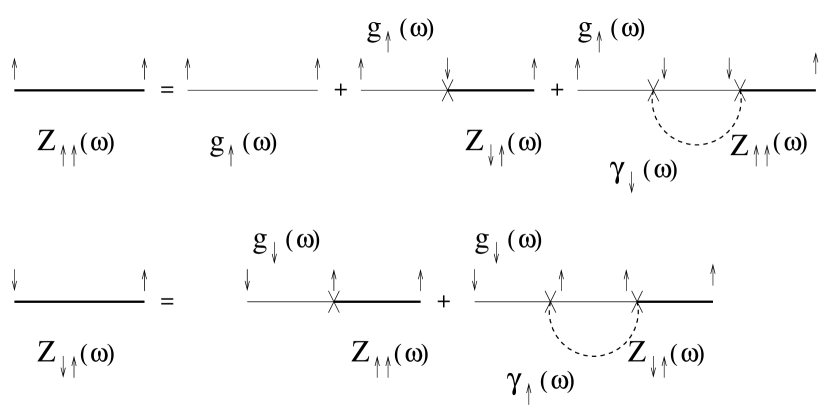
Figure 7: Diagrams contributing to the Dyson equations for ${\bf Z}_{\uparrow\uparrow}$ and for ${\bf Z}_{\downarrow\uparrow}$.

$${\bf Z}_{\sigma\sigma}(\omega)\approx\frac{i(\omega-\omega_{0})+E_{\bar{\sigma}}(\vec{\beta})}{[i(\omega-\omega_{0})+E_{\sigma}(\vec{\beta})][i(\omega-\omega_{0})+E_{\bar{\bar{\sigma}}}(\vec{\beta})]-Y^{2}}\>\>\>\>.$$ (68)

The partition function is then given by

$${\bf Z}[\mu_{1},\mu_{2}^{*}]\approx 2\exp\left\{-\beta\frac{g\pi v}{L}\left[\left(\frac{\mu_{1}}{2\pi}\right)^{2}+\left(\frac{\mu_{2}-\mu_{2}^{*}}{2\pi}\right)^{2}+\frac{1}{3}-\sqrt{\left(\frac{\mu_{2}-\mu_{2}^{*}}{2\pi}\right)^{2}+\frac{y^{2}}{2\pi vg}}\right]\right\}\>,$$ (69)

with $y=LY\sim L^{1-h_{S}(g)}$. From Eq.(69), one may derive the Josephson current distribution in the three arms of the YJJN

$$I_{1} = \frac{e^{*}v}{L}\left\{\frac{1}{\sqrt{2}}\left(\frac{\mu_{1}}{2\pi}\right)+\frac{1}{\sqrt{6}}\left(\frac{\mu_{2}-\mu_{2}^{*}}{2\pi}\right)\left[1+\frac{1}{2}\left[\left(\frac{\mu_{2}-\mu_{2}^{*}}{2\pi}\right)^{2}+\left(\frac{y}{\pi vg}\right)^{2}\right]^{-\frac{1}{2}}\right]\right\}$$

$$I_{2} = \frac{e^{*}v}{L}\left\{-\frac{1}{\sqrt{2}}\left(\frac{\mu_{1}}{2\pi}\right)+\frac{1}{\sqrt{6}}\left(\frac{\mu_{2}-\mu_{2}^{*}}{2\pi}\right)\left[1+\frac{1}{2}\left[\left(\frac{\mu_{2}-\mu_{2}^{*}}{2\pi}\right)^{2}+\left(\frac{y}{\pi vg}\right)^{2}\right]^{-\frac{1}{2}}\right]\right\}$$

$$I_{3} = -\frac{e^{*}v}{L}\sqrt{\frac{2}{3}}\left(\frac{\mu_{2}-\mu_{2}^{*}}{2\pi}\right)\left[1+\frac{1}{2}\left[\left(\frac{\mu_{2}-\mu_{2}^{*}}{2\pi}\right)^{2}+\left(\frac{y}{\pi vg}\right)^{2}\right]^{-\frac{1}{2}}\right]\>\>\>\>.$$ (70)

The formalism developed in this appendix allows also to compute the (transverse part of the) dynamical spin susceptibility of the emerging two-level system, $\chi_{\perp}(\Omega)$. As discussed in section 5, the imaginary part of $\chi_{\perp}(\Omega)/\Omega$ is the place to look at, in order to analyze the entanglement between the system and the environmental modes.

The starting point to derive the _xx and the _yy-components of $\chi_{\perp}(\Omega)$ is the computation of $\chi_{\perp}^{+-}(\Omega)$ and $\chi_{\perp}^{-+}(\Omega)$, that is, of the Fourier transforms of the imaginary time dynamical susceptibilities $\chi_{\perp}^{+-}(\tau)$, and $\chi_{\perp}^{-+}(\tau)$, respectively given by

$$\chi_{\perp}^{+-}(\tau)=\langle{\bf T}_{\tau}[\sigma^{+}(\tau)\sigma^{-}(0)]\rangle\;\;\;,\;\;\chi_{\perp}^{-+}(\tau)=\langle{\bf T}_{\tau}[\sigma^{-}(\tau)\sigma^{+}(0)]\rangle\;\;\;\>.$$ (71)

The approximate computation of $\chi_{\perp}^{+-}(\Omega)$ is graphically shown in Fig.8a). To lowest order in $Y$, $\chi_{\perp}^{+-}(\Omega)$ is computed as a loop defined by the $|\uparrow\rangle$-state propagating forward in (imaginary) time, and by the $|\downarrow\rangle$-state propagating backward, while $\chi_{\perp}^{-+}(\Omega)$ is computed in the same way, by just exchanging $\uparrow$ and $\downarrow$. Accordingly, $\chi_{\perp}^{+-}(\Omega)$ and $\chi_{\perp}^{-+}(\Omega)$, are given by

$$[\chi_{\perp}^{+-}]^{(0)}(i\Omega)\approx\int\>\frac{d\omega}{2\pi}\>{\bf Z}_{\uparrow\uparrow}(\omega){\bf Z}_{\downarrow\downarrow}(\omega+\Omega)\;,\;[\chi_{\perp}^{-+}]^{(0)}(i\Omega)\approx\int\>\frac{d\omega}{2\pi}\>{\bf Z}_{\uparrow\uparrow}(\omega+\Omega){\bf Z}_{\downarrow\downarrow}(\omega)\>,$$ (72)

where the functions ${\bf Z}_{\sigma\sigma}(\omega)$ have been defined in Eq.(68). As a result, one obtains

$$[\chi_{\perp}^{+-}]^{(0)}(i\Omega)=\frac{i\Omega[\Delta(\vec{\mu})+E_{\downarrow}(\vec{\mu})]-Y^{2}}{4\Delta^{2}(\vec{\mu})}\frac{1}{i\Omega-2\Delta(\vec{\mu})}$$

$$+\frac{i\Omega[\Delta(\vec{\mu})+E_{\uparrow}(\vec{\mu})]-Y^{2}}{4\Delta^{2}(\vec{\mu})}\frac{1}{i\Omega+2\Delta(\vec{\mu})}\>\>\>\>,$$ (73)

with $\Delta(\vec{\mu})=\sqrt{[E_{\uparrow}(\vec{\mu})]^{2}+Y^{2}}$. A similar formula holds for $[\chi_{\perp}^{+-}]^{(0)}(i\Omega)$, provided one exchanges $\uparrow$ with $\downarrow$, and vice versa, in Eq.(73). For $1<g<9/4$ and $\gamma\neq(2k+1)\pi/3$, and for $g>9/4$, one may safely neglect higher order corrections in $Y$ to $\chi_{\perp}(\Omega)$, so that Eq.(73) provides a reliable estimate of the transverse dynamical spin susceptibility. Both the _xx and the _yy components of $\chi_{\perp}(\Omega)$ are obtained from Eq.(73), and from the analogous one for $\chi_{\perp}^{-+}(\Omega)$. Their imaginary part is computed via the replacement $\Omega\longrightarrow-i\Omega+0^{+}$: in both cases it is equal to $\chi^{``}_{\perp}(\Omega)$, given by

$$\frac{\chi^{``}_{\perp}(\Omega)}{\Omega}\propto\delta(\Omega-2\Delta(\vec{\mu}))+\delta(\Omega+2\Delta(\vec{\beta}))\>\>\>\>.$$ (74)

Eq.(74) is the estimate of $\chi^{``}_{\perp}(\Omega)/\Omega$ near the SFP, quoted in section 5.1.

For $g<1$, the instantons provide a relevant perturbation: thus, higher-order contribution in $Y$ to Eq.(72) cannot be neglected. By taking the large-$Y$ limit of the fully dressed expression for ${\bf Z}_{\sigma\sigma}(\omega)$ derived in Eq.(67), one gets, for the imaginary part of the transverse dynamical spin susceptibility

$$\frac{\chi^{``}_{\perp}(\Omega)}{\Omega}\propto[|2E_{\uparrow}(\vec{\mu})+\Omega|^{3-\frac{16}{9}g}-|2E_{\uparrow}(\vec{\mu})-\Omega|^{3-\frac{16}{9}g}]/\Omega\>\>\>\>.$$ (75)

Eq.(75) shows that the largest part of the spectral weight is now in the region around $\Omega=0$: this signals the onset of a fully entangled state between the two state system and the bath formed by the plasmon modes [21, 22].

For $1<g<9/4$ and $\gamma=(2k+1)\pi/3$, the behavior of the system is ruled by the IR stable FFP. An estimate of $\chi_{\perp}^{+-}(\Omega)$ may now be done, for instance, when $g=\frac{9}{4}-\epsilon$, with $\epsilon\ll 1$: since the FFP is at $\zeta_{*}\sim\epsilon^{\frac{1}{2}}$, using the effective Hamiltonian in Eq.(47), one may resort to the RPA computation of the dynamical spin susceptibility, graphically drawn in Fig.8b), to get

$$[\chi_{\perp}^{+-}]_{\rm RPA}(\Omega)\approx\frac{1}{\Omega-\Delta_{*}(\vec{\mu})-\zeta^{2}\Gamma[-1-\frac{8}{9}\epsilon](-\Omega)^{1+\frac{8}{9}\epsilon}}$$

$$+\frac{1}{\Omega+\Delta_{*}(\vec{\beta})-\zeta^{2}\Gamma[-1-\frac{8}{9}\epsilon](-\Omega)^{1+\frac{8}{9}\epsilon}}\>\>\>\>,$$ (76)

with $\Delta_{*}(\vec{\mu})=\sqrt{[E_{\uparrow}(\vec{\beta})]^{2}+(\zeta_{*}/L)^{2}}$. Computing $\chi^{``}(\Omega)/\Omega$ From Eq.(76), one sees that, on one hand, the energies of the two-level quantum system are renormalized by $\zeta$ to $\pm\Delta_{*}(\vec{\mu})$, on the other hand, that the two peaks at the renormalized energies now display a finite width $\propto\frac{\pi v}{L}(\zeta_{*})^{1+\frac{8}{9}g}$, which is the result quoted in section 5.2.

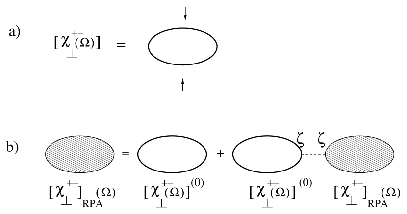
Figure 8: Diagrams contributing to the RPA computation of the dynamical spin susceptibility: the dashed line represents the propagation of the W-instanton.

References

- [1] C. Chamon, M. Oshikawa and I. Affleck, Phys. Rev. Lett. 91, (2003), 206403; M. Oshikawa, C. Chamon and I. Affleck, Journal of Statistical Mechanics JSTAT/2006/P02008; Chang-Yu Hou and Claudio Chamon, Phys. Rev. B 77, (2008), 155422.
- [2] A. Tokuno, M. Oshikawa and E. Demler, Phys. Rev. Lett. 100, (2008), 140402.
- [3] K. Kazymyrenko and B. Douçot, Phys. Rev. B 71, (2005), 075110; K. Kazymyrenko, S. Dusuel, and B. Douçot, Phys. Rev. B 72, (2005), 235114; S. Lal, S. Rao and D. Sen, Phys. Rev. B 66 (2002), 165327; S. Das, S. Rao and D. Sen, Phys. Rev. B 70 (2004), 085318; Phys. Rev. B 74 (2006), 045322; V. R. Chandra, S. Rao, and D. Sen, Phys. Rev. B 75, (2007), 045435; S. Das and S. Rao, arXiv preprint/0807.0804.
- [4] H. Guo and S. R. White, Phys. Rev. B 74, (2006), 060401(R).
- [5] S. A. Reyes and A. M. Tsvelik, Phys. Rev. 95, (2005), 186404.
- [6] A. M. Tsvelik and P. B. Wiegmann, Adv. Phys. 32, (1983), 453; P. Schlottmann, Phys. Rep. 181, (1989), 1; P. Nozieres and A. Blandin, J. Phys. (France), 41, (1980), 193; I. Affleck and A. W. Ludwig, Phys. Rev. B 48, (1993), 7297.
- [7] S. Eggert and I. Affleck, Phys. Rev. B 46, (1992), 10866.
- [8] P. Fendley. A. W. W. Ludwig, and H. Saleur, Phys. Rev. Lett. 74, (1995), 3005; A. M. Chang, Rev. Mod. Phys. 75, (2003), 1449.
- [9] See, for instance, A. O. Gogolin, A. A. Nersesyan, and A. M. Tsvelik, Bosonization and Strongly Correlated Systems, Cambridge University Press. (2004).
- [10] C.L. Kane and M. P. Fisher, Phys. Rev. Lett. 68, (1992), 1220; Phys. Rev. B46, (1992), 15233.
- [11] D. Giuliano and P. Sodano, Nucl. Phys. B 711, (2005), 480.
- [12] D. Giuliano and P. Sodano, Nucl. Phys. B 770, (2007), 332.
- [13] L. I. Glazman and A. I. Larkin, Phys. Rev. Lett. 79, 3736-3739 (1997).
- [14] F. W. J. Hekking and L. I. Glazman, Phys. Rev. B 55, (1997), 6551.
- [15] H.Yi and C.L.Kane, Phys.Rev.B 57,R5579-R5582(1998).
- [16] I. Affleck, M. Oshikawa and H. Saleur, Nucl. Phys. B594, (2001), 535.
- [17] Y. Makhlin, G. Shön, and A. Shnirman, Rev. Mod. Phys. 73, (2001), 357.
- [18] J. R. Schrieffer and P. A. Wolff, Phys. Rev. 149, (1966), 491.
- [19] J. M. Luttinger, J. Math. Phys. 4, (1963) 1154; S. Tomonaga, Prog. Theor. Phys. 5, (1950) 544.
- [20] See, for example, P. Ginsparg, “Applied Conformal Field Theory”, in Field, Strings and Critical Phenomena, Les Houches, Section XLIX, (1988), Edited by E. Brézin and P. Zinn-Justin.
- [21] D. Giuliano and P. Sodano, New Journal of Physics 10, (2008) 093023.
- [22] E. Novais, A. H. Castro Neto, L. Borda, I. Affleck, and G. Zarand, Phys. Rev. B 72, (2005), 014417.
- [23] C. Granata, A. Vettoliere and M. Russo, Appl. Phys. Lett. 88, (2006) 212506.
- [24] D. B. Haviland, K. Andersson, and P. Agren, J. Low Temp. Phys. 124,(2001) 291.
- [25] M. V. Feigel’man, L. B. Ioffe, V. B. Geshkenbern, P. Dayal, and G. Blatter, Phys. Rev. Lett 92, 098301 (2004); Phys. Rev. B 70, 224524 (2004).
- [26] S. Fubini and G. Veneziano, Nuovo Cimento A67, 29 (1970); Ann. Phys. 63, 12 (1970).