Quantum properties of a superposition of squeezed displaced two-mode vacuum and single-photon states

Abstract

In this paper, we study some quantum properties of a superposition of displaced squeezed two-mode vacuum and single-photon states, such as the second-order correlation function, the Cauchy-Schwartz inequality, quadrature squeezing, quasiprobability distribution functions and purity. This type of states includes two mechanisms, namely, interference in phase space and entanglement. We show that these states can exhibit sub-Piossonian statistics, squeezing and deviate from the classical Cauchy-Schwartz inequality. Moreover, the amount of entanglement in the system can be increased by increasing the squeezing mechanism. In the framework of the quasiprobability distribution functions we show that the single-mode state can tend to thermal state based on the correlation mechanism. Generation scheme for such states is given.

I Introduction

Developing new states beside the traditional ones is an important topic in quantum optics and quantum information theories. Fock state $|n\rangle$ and coherent state $|\alpha\rangle$ are the most commonly used states in these theories. The single-mode squeezed states of electromagnetic field are purely quantum states since they have less uncertainty in one quadrature than the vacuum noise level. Additionally, these states exhibit a variety of nonclassical effects, e.g. sub-Poissonian statistics har and oscillatory behavior in the photon-number distribution pho . These states can be generated via a degenerate parametric amplifier wu . The third type of states given in the literature is the two-mode squeezed states two , which contain quantum correlations between two different modes of the field. The importance of these states comes from their connection to the two-photon nonlinear processes, e.g. non-degenerate parametric amplifier dege . These states have been used in the continuous-variable teleportation [7] , quantum key distribution [9] , verification of EPR correlations [12] , etc. The single-mode state–obtained from the two-mode squeezed state by tracing out the other mode–cannot exhibit squeezing bern ; rabha1 . Precisely, because of the correlation between modes in the two-mode squeezed operator, the squeezing of the quantum fluctuations does not occur in the individual modes but it occurs in the superposition of the two modes.

A great attention has been devoted to produce mesoscopic superposition states. These states have interesting distinct characteristics than the classical ones such as interference in phase space, squeezing and quantum entanglement quan1 . These remarkable properties present the mesoscopic superposition states as powerful tools in quantum information processing, metrology raimond ; Glancy and experimental studies of decoherence zurek . The most famous superimposed state in the literature is the Schrödinger-cat state sch1 . There are several proposals for generating superposition of optical coherent states in the literature. For recent review the reader can consult Glancy and the references cited therein. Besides the Schrödinger-cat states various types of superposition have been developed, e.g. the superposition of squeezed and displaced number states without oba1 and with thermal noise elo1 . Moreover, the superposition of multiple mesoscopic states is given in agar , and has been generated using resonant interaction between atoms and the field in a high quality cavity. The superposition of the two-mode states is discussed in chin . These states–under certain conditions become very close to the well-known Bell-states quan1 and they can be generated by a resonant bichromatic excitation of $N$ trapped ions solano . The entanglement of a superposition of two bipartite states in terms of the correlation of the two states constituting the superposition has been discussed in gilad .

Developing new states is an important topic for understanding the boundary between the classical and quantum mechanics as well as to cover the needs of the progress in the quantum information theory. Moreover, the investigation of nonclassical effects of the quantum states is of considerable and continuing interest, since it plays an important role both fundamentally and practically in the quantum information theory. Throughout this paper we study the quantum properties of the superposition of squeezed displaced two-mode number states (STDSN), in particular, the vacuum and single-photon states. In these states the squeezing mechanism is involved via non-degenerate squeezed operator. These states are different from the superposition of the single-mode states oba1 ; elo1 in the following sense: They include two mechanisms: (i) entanglement and/or correlation between the two-modes. (ii) Two-mode interferences in phase space. These states can be generated via two-mode trapped ions trapa , as we will show in section VI. For STDSN we study the single-mode second-order correlation, Cauchy-Schwartz inequality, quadrature squeezing, quasiprobability functions and purity. We show that the nonclassical effects are remarkable in the different quantities. Also the single-mode state tends to the thermal state based on the correlation mechanism and the amount of entanglement can be increased by increasing the squeezing mechanism.

We perform this investigation in the following order. In section II we introduce the state formalism and comment on its photon-number distribution. In section III we discuss the second-order correlation function and Cauchy-Schwartz inequality. In section IV the quadrature squeezing in the framework of principal squeezing is investigated. In section V quasiprobability distribution functions and the purity are investigated. The generation of the STDSN is discussed in section VI, however, the conclusions are summarized in section VII.

II State formalism

The correlated two-mode squeezed states are connected with the two-mode squeeze operator, which has the form:

$$\hat{S}(r)=\exp[\frac{r}{2}(\hat{a}\hat{b}-\hat{a}^{{\dagger}}\hat{b}^{{\dagger}})],$$ (1)

where $\hat{a}\quad(\hat{a}^{\dagger})$ and $\hat{b}\quad(\hat{b}^{\dagger})$ denote the annihilation (creation) operators of the first (signal) and second (idler) mode, respectively. By means of this operator and the superposition principle we develop a new class of states, namely, superposition of squeezed displaced two-mode number states (STDSN) as:

$$|\psi\rangle=|r,\alpha,\beta\rangle_{\epsilon}=\lambda_{\epsilon}[\hat{D}(\alpha_{1},\alpha_{2})+\epsilon\hat{D}(-\alpha_{1},-\alpha_{2})]\hat{S}(r)|n,m\rangle,$$ (2)

where $\epsilon=|\epsilon|\exp(i\phi),\hat{S}(r)$ is given by (1) and $\hat{D}(\alpha_{1},\alpha_{2})$ is the two-mode displaced operator defined as:

$$\hat{D}(\alpha_{1},\alpha_{2})=\hat{D}(\alpha_{1})\hat{D}(\alpha_{2})=\exp(\alpha_{1}\hat{a}^{{\dagger}}-\alpha_{1}^{*}\hat{a})\exp(\alpha_{2}\hat{b}^{{\dagger}}-\alpha_{2}^{*}\hat{b})$$ (3)

and $\alpha_{j}$ is generally a complex parameter (a field amplitude), however, throughout the investigation in this paper it will be considered real. Also the prefactor $\lambda_{\epsilon}$ is the normalization constant, which can be easily evaluated as:

$$|\lambda_{\epsilon}|^{-2}=1+|\epsilon|^{2}+2|\epsilon|\mu{\rm L}_{n}(4t_{1}^{2}){\rm L}_{m}(4t_{2}^{2})\cos\phi,$$ (4)

where

$$t_{1}=\alpha_{1}C_{r}+\alpha_{2}S_{r},\quad t_{2}=\alpha_{2}C_{r}+\alpha_{1}S_{r},\quad S_{r}=\sinh r,C_{r}=\cosh r,\quad\mu=\exp[-2(t^{2}_{1}+t^{2}_{2})]$$ (5)

and ${\rm L}_{n}(.)$ is the Laguerre polynomial of order $n$ (see (8) below). Throughout the paper we study only two choices for the parameter $|\epsilon|$, namely, $1$ and $0$, however, for the parameter $\phi$ we take the values $0,\pi$ and $\pi/2$. Precisely, when $|\epsilon|=1$ and $\phi=0,\pi,\pi/2$ the states (2) are called even-type, odd-type and Yurke-type states, respectively.

When $|n,m\rangle=|0,0\rangle$ the states (2) can be expressed in a closed form in terms of the Fock states cave as:

$$|\psi\rangle=\sum\limits_{n_{1},n_{2}=0}^{\infty}C(n_{1},n_{2})|n_{1},n_{2}\rangle,$$ (6)

where

$$\begin{array}[]{lr}C(n_{1},n_{2})=\lambda_{\epsilon}[1+(-1)^{n_{1}+n_{2}}\epsilon]\frac{1}{\cosh r}\exp[-\frac{1}{2}(\alpha_{1}\mu_{1}+\alpha_{2}\mu_{2})]\sqrt{\frac{M!}{N!}}(\mu_{1})^{n_{1}-M}(\mu_{2})^{n_{2}-M}\\ \\ \times(\tanh r)^{M}{\rm L_{M}^{N-M}}\left(-\frac{\mu_{1}\mu_{2}}{\tanh r}\right),\\ \\ \mu_{1}=\alpha_{1}-\alpha_{2}\tanh r,\quad\mu_{2}=\alpha_{2}-\alpha_{1}\tanh r,\quad M=min(n_{1},n_{2}),\quad N=max(n_{1},n_{2})\end{array}$$ (12)

and ${\rm L}_{k}^{\upsilon}(.)$ is the associated Laguerre polynomial having the form:

$${\rm L}_{k}^{\upsilon}(x)=\sum\limits_{l=0}^{k}\frac{(\upsilon+k)!(-x)^{l}}{(\upsilon+l)!(k-l)!l!}.$$ (13)

The photon-number distribution of (6) can be evaluated as:

$$P(m_{1},m_{2})=|C(m_{1},m_{2})|^{2},$$ (14)

where $C(m_{1},m_{2})$ is given by (12). It is obvious that $P(m_{1},m_{2})$ can exhibit pairwise oscillations based on the values of the sum $m_{1}+m_{2}$, even if $r=0$. We have to remark that the components of the STDSN can exhibit oscillatory behavior in $P(m_{1},m_{2})$ cave , apart from the superposition mechanism, which can make this behavior more or less pronounced. Moreover, the single-mode photon-number distribution can be obtained via the relation:

$$P(m_{1})=\sum\limits_{m_{2}=0}^{\infty}|C(m_{1},m_{2})|^{2}.$$ (15)

In $P(m_{1})$ the occurrence of the oscillatory behavior results from the interference mechanism. We can explain this fact for the simplest case $r=0,n=m=0,\epsilon=\exp(i\phi)$ and hence (15) reduces to

$$P(m_{1})=2|\lambda_{\epsilon}|^{2}\exp(-\alpha_{1}^{2})\frac{\alpha_{1}^{2m_{1}}}{m_{1}!}[1+(-1)^{m_{1}}\exp(-2\alpha_{2}^{2})\cos\phi].$$ (16)

The oscillatory behavior in $P(m_{1})$ depends on the values of $\alpha_{2}$ and $\phi$, i.e. for large values of $\alpha_{2}$, $P(m_{1})$ tends to that of the coherent state. This means that one can use the second mode to control the nonclassical effects in the first mode and vice versa.

In the following sections we investigate the properties of the state (2). For the sake of simplicity we treat the second-order correlation function, Cauchy-Schwartz inequality, squeezing and purity using the form (6) (,i.e., $|n,m\rangle=|0,0\rangle$), however, the quasiprobability functions are given for the case $|n,m\rangle=|0,1\rangle$. This is to estimate a global information on the generic form.

III Second-order correlation function and Cauchy-Schwartz inequality

In this section we investigate the behavior of the second-order correlation function and Cauchy-Schwartz inequality for the state (6). These two quantities can give information on the correlation between the modes in the quantum system. The second-order correlation function for the first mode, e.g. $\hat{a}$, is defined by

$$g^{(2)}(0)=\frac{\langle\hat{a}^{\dagger 2}\hat{a}^{2}\rangle}{\langle\hat{a}^{\dagger}\hat{a}\rangle^{2}}-1,$$ (17)

where $g^{(2)}(0)=0$ for Poissonian statistics (standard case), $g^{(2)}(0)<0$ for sub-Poissonian statistics (nonclassical effects) and $g^{(2)}(0)>0$ for super-Poissonian statistics (classical effects). The second-order correlation function can be measured by a set of two detectors mandl , e.g. the standard Hanbury Brown-Twiss coincidence arrangement. For this quantity we restrict the discussion to the first-mode only. For this mode one can easily obtain:

$$\langle\hat{a}^{{\dagger}}\hat{a}\rangle=|\lambda_{\epsilon}|^{2}\{(S_{r}^{2}+\alpha_{1}^{2})(1+|\epsilon|^{2})+2|\epsilon|\mu\cos\phi\left[S^{2}_{r}-4t_{1}t_{2}S_{r}C_{r}+2\alpha_{1}t_{2}S_{r}-2\alpha_{1}t_{1}C_{r}+\alpha_{1}^{2}\right]\},$$ (18)

$$\begin{array}[]{lr}\langle\hat{a}^{{\dagger}2}\hat{a}^{2}\rangle=|\lambda_{\epsilon}|^{2}\{(\alpha_{1}^{4}+2S^{4}_{r}+4\alpha_{1}^{2}S^{2}_{r})(1+|\epsilon|^{2})+2|\epsilon|\mu\cos\phi\left[4\alpha^{2}_{1}C_{r}^{2}t^{2}_{1}+16S_{r}^{2}C_{r}^{2}t^{2}_{1}t^{2}_{2}\right.\\ +16\alpha_{1}S_{r}C_{r}^{2}t^{2}_{1}t_{2}+\alpha^{4}_{1}+4\alpha^{2}_{1}S_{r}^{2}t^{2}_{2}+2S_{r}^{4}+8\alpha_{1}S_{r}^{3}t_{2}+4\alpha^{3}_{1}S_{r}t_{2}-8\alpha^{2}_{1}S_{r}^{2}t_{2}-4\alpha^{3}_{1}C_{r}t_{1}\\ \left.-16\alpha_{1}S_{r}^{2}C_{r}t_{1}t^{2}_{2}-16S_{r}^{3}C_{r}t_{1}t_{2}-16\alpha^{2}_{1}S_{r}C_{r}t_{1}t_{2}-8\alpha_{1}S_{r}^{2}C_{r}t_{1}\right]\}.\end{array}$$ (22)

It is worth mentioning that the most general cases for equations (18) and (22) have been given in mank for the multimode squeezed cat states but with different parameterizations.

Substituting (18), (22) into (17) and taking $r=0$ we obtain

$$g^{(2)}(0)=\frac{[1+|\epsilon|^{2}+2|\epsilon|\exp[-2(\alpha_{1}^{2}+\alpha_{2}^{2})]\cos\phi]^{2}}{[1+|\epsilon|^{2}-2|\epsilon|\exp[-2(\alpha_{1}^{2}+\alpha_{2}^{2})]\cos\phi]^{2}}-1.$$ (23)

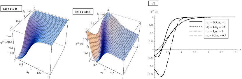
Figure 1: The second-order correlation function of the first mode for $(|\epsilon|,\phi)=(1,\pi)$ against $(\alpha_{1},\alpha_{2})$ (a)–(b) and $r$ (c) for different values of the parameters as indicated.

From (23) it is obvious that the sub-Poissonian statistics can occur only for $\phi=\pi$ and $2(\alpha_{1}^{2}+\alpha_{2}^{2})$ being small. This means that the odd-type state can exhibit nonclassical effects in the framework of $g^{(2)}(0)$. In this case, the mode under consideration reduces to the standard odd-coherent state with the components $|\pm\sqrt{\alpha_{1}^{2}+\alpha_{2}^{2}}\rangle$. The obvious remark is: when the mode $\hat{a}$ is prepared in the vacuum state $|0\rangle$, its $g^{(2)}(0)$ can exhibit sub-Poissonian statistics based on the values of $\alpha_{2}$ of the second mode. Similar argument can be given to the second mode. This reflects the role of the correlation between the modes in the system, which leads to the possibilities of controlling one mode by the other one. Now we draw the attention to the general case when the squeezing mechanism is involved. We have noted that the even-type and the Yurke-type states cannot exhibit sub-Poissonian statistics. Information about $g^{(2)}(0)$ of the odd-type states is depicted in Figs. 1(a)–(c) for given values of the parameters $\alpha_{1}$ and $\alpha_{2}$. From Fig. 1(a) one can observe the occurrence of the sub-Poissonian statistics, in particular, for small values of $\alpha^{,}s$. When the squeezing mechanism is involved, the amounts of the nonclassical effects in $g^{(2)}(0)$ decrease and eventually vanish for large value of $r$ (see Fig. 1(b)). For $\alpha_{1}=\alpha_{2}=0$ and $r\neq 0$ state (6) reduces to the two-mode squeezed vacuum state. In this case we have $g^{(2)}(0)=1$, which is independent of $r$. This is remarkable in Fig. 1(b), which shows sub-Poissonian statistics only when one or both of $\alpha_{j}>0$. Fig. 1(c) gives the range of the parameter $r$ (for certain values of $\alpha_{j}$) for which the sub-Piossonian statistics occur. It is obvious that the smaller the values of $\alpha_{j}$, the greater this range is.

Figure 2: The factor $V$ against the parameter $r$ for $(|\epsilon|,\phi,\alpha_{1})=(1,\pi/2,0.5)$ (a) and $(1,\pi,0.5)$ (b) for $\alpha_{2}=0.2$ (solid), $0.3$ (short-dashed curve), $0.4$ (long-dashed curve) and $0.5$ (star-centered curve).

We conclude this section by investigating the intermodal correlations in terms of the deviation from the classical Cauchy-Schwarz inequality. Classically, Cauchy-Schwarz inequality has the form [32] :

$$\langle I_{1}I_{2}\rangle\leq\langle I_{1}\rangle\langle I_{2}\rangle,$$ (24)

where $I_{j},j=1,2$ are classical intensities of light measured by different detectors in a double-beam experiment. In quantum theory, the deviation from this classical inequality can be represented as $V<0$, where the factor $V$ takes the form agrw :

$$V=\frac{\sqrt{\langle\hat{a}^{{\dagger}2}\hat{a}^{2}\rangle\langle\hat{b}^{{\dagger}2}\hat{b}^{2}\rangle}}{\langle\hat{a}^{{\dagger}}\hat{b}^{{\dagger}}\hat{a}\hat{b}\rangle}-1.$$ (25)

Occurrence of negative values in $V$ means that the intermodal correlation is larger than the correlation between photons in the same mode kinn and this indicates strong deviation from the classical Cauchy-Schwartz inequality. The origin in this deviation is that in the quantum mechanical treatment we involve pseudodistributions instead of the true ones. This implies that the Glauber-Sudarshan $P$-function possesses strong quantum properties agrw . Moreover, the deviation from the Cauchy-Schwarz inequality can be observed in a two-photon interference experiment mand . For completeness, the expectation value $\langle\hat{a}^{{\dagger}}\hat{b}^{{\dagger}}\hat{a}\hat{b}\rangle$ for the state (6) can be easily evaluated as:

$$\begin{array}[]{lr}\langle\hat{a}^{{\dagger}}\hat{a}\hat{b}^{{\dagger}}\hat{b}\rangle=|\lambda_{\epsilon}|^{2}\left\{[S^{4}_{r}+(S_{r}C_{r}-\alpha_{1}\alpha_{2})^{2}+(\alpha_{1}^{2}+\alpha_{2}^{2})S^{2}_{r}](1+|\epsilon|^{2})\right.\\ \\ +2|\epsilon|\mu\cos\phi\left[S^{2}_{r}\cosh(2r)-\alpha_{1}\alpha_{2}\sinh(2r)+(\alpha_{2}^{2}+\alpha_{1}^{2})S_{r}^{2}\right.\\ \\ -2t_{1}t_{2}[\sinh(2r)(2S^{2}_{r}+\alpha^{2}_{1}+\alpha^{2}_{2}+\cosh(2r))-2\alpha_{1}\alpha_{2}\cosh(2r)]+4\sinh^{2}(2r)t^{2}_{1}t^{2}_{2}\\ \\ +2t_{2}[-S_{r}\sinh(2r)\alpha_{2}+\alpha_{1}S_{r}\cosh(2r)-\alpha_{1}\alpha_{2}(\alpha_{1}C_{r}-\alpha_{2}S_{r})]\\ \\ -2t_{1}[(\alpha_{1}C_{r}-\alpha_{2}S_{r})S^{2}_{r}+(\alpha_{1}S_{r}-\alpha_{2}C_{r})(S_{r}C_{r}-\alpha_{1}\alpha_{2})]\\ \\ -\left.4\sinh(2r)(\alpha_{1}C_{r}-\alpha_{2}S_{r})(t_{2}-t_{1})t_{1}t_{2}-2\alpha_{1}\alpha_{2}\sinh(2r)(t^{2}_{1}+t^{2}_{2})+\alpha^{2}_{1}\alpha^{2}_{2}\right\}.\end{array}$$ (37)

The expectation value $\langle\hat{b}^{{\dagger}2}\hat{b}^{2}\rangle$ can be obtained from (22) using the interchange $\alpha_{1}\longleftrightarrow\alpha_{2}$. One can easily find $V=0$ for $r=0$. Generally, we have noted that $V<0$ only when $\alpha_{j}$ are small (see Figs. 2). Fig. 2(a) is given for the Yurke-type state which is identical to that of the two-mode squeezed displaced states (cf. (22) and (37) for $\phi=\pi/2$). From these figures the strongest deviation from the classical inequality occurs for $\alpha_{j}(\neq 0)$ and $r$ small, i.e. the photons are more strongly correlated than it is classically possible, and then the curve monotonically increases as $r$ increases. As the values of $\alpha_{2}$ increase the negative values in the factor $V$ decrease and eventually disappear (compare different curves in these figures). Also a comparison between Fig. 2(a) and Fig. 2(b) shows that the nonclassical effects occurred in the factor $V$ for the odd-type state are greater than those in the state with Yurke-type state.

IV Quadrature squeezing

In this section we discuss the quadrature squeezing for the state under consideration. As it is well known, the quadrature squeezing can be measured by a homodyne detector in which the signal is superimposed on a strong coherent beam of the local oscillator homo . Here we use the notion of the principal squeezing princ , which can give one form for the single-mode and two-mode cases. In this respect, we define the two quadratures in the following forms:

$$\hat{X}=\hat{X}_{1}\cos\nu+\hat{X}_{2}\sin\nu,\quad\hat{Y}=\hat{Y}_{1}\cos\nu+\hat{Y}_{2}\sin\nu,$$ (38)

where the subscripts $1$ and $2$ stand for the first and second mode, respectively, and $\nu$ is a rotation angle. When $\nu=0,\pi/2,\pi/4$ the quadratures (38) yield those of the first mode, second mode and compound modes, respectively. For the first mode the quadrature operators can be defined as:

$$\hat{X}_{1}=\frac{1}{2}\left(\hat{a}+\hat{a}^{{\dagger}}\right),\quad\hat{Y}_{1}=\frac{1}{2i}\left(\hat{a}-\hat{a}^{{\dagger}}\right).$$ (39)

Similar definition can be quoted for the second mode via the interchange $\hat{a}\longrightarrow\hat{b}$. The quadratures (38) satisfy the following commutation rule:

$$\left[\hat{X},\hat{Y}\right]=\frac{i}{2}.$$ (40)

Therefore, the squeezing factors associated with the $\hat{X}$ and $\hat{Y}$ can be expressed as:

Figure 3: Squeezing factor $S$ for $(|\epsilon|,\phi)=(1,0)$ with $(r,\alpha_{1},\alpha_{2})=(0,\alpha,\alpha)$ (a) and $\alpha_{1}=\alpha_{2}=0.6$ (b).

$$\begin{array}[]{lr}F=\langle(\vartriangle\hat{X})^{2}\rangle-1\\ \\ =F_{1}\cos^{2}\nu+F_{2}\sin^{2}\nu+F_{c}\sin(2\nu),\\ \\ S=\langle(\vartriangle\hat{Y})^{2}\rangle-1\\ \\ =S_{1}\cos^{2}\nu+S_{2}\sin^{2}\nu+S_{c}\sin(2\nu).\end{array}$$ (48)

where $F_{j},S_{j},j=1,2,c$, take the forms:

$$\begin{array}[]{lr}F_{1}=2S_{r}^{2}+4\alpha_{1}^{2}|\lambda_{\epsilon}|^{2}[1+|\epsilon|^{2}-|\lambda_{\epsilon}|^{2}(1-|\epsilon|^{2})^{2}],\\ \\ S_{1}=2S_{r}^{2}-4|\lambda_{\epsilon}|^{2}|\epsilon|\mu(\alpha_{1}^{2}+4t_{1}t_{2}S_{r}C_{r})\cos\phi\\ \\ -4|\lambda_{\epsilon}|^{2}|\epsilon|\mu(2t_{1}C_{r}-\alpha_{1})^{2}\left(\cos\phi+4|\lambda_{\epsilon}|^{2}|\epsilon|^{2}\mu\sin^{2}\phi\right),\\ \\ F_{c}=4\alpha_{1}\alpha_{2}-2S_{r}C_{r}-8\alpha_{1}\alpha_{2}|\epsilon|\mu|\lambda_{\epsilon}|^{2}\cos\phi-4|\lambda_{\epsilon}|^{2}(1-|\epsilon|^{2})^{2}\alpha_{1}\alpha_{2},\\ \\ S_{c}=2C_{r}S_{r}-8|\epsilon||\lambda_{\epsilon}|^{2}\mu(2t_{1}C_{r}-\alpha_{1})(t_{1}S_{r}+t_{2}C_{r})\cos\phi-16|\epsilon|^{2}|\lambda_{\epsilon}|^{4}\mu^{2}(\alpha_{1}-2t_{1}C_{r})(\alpha_{2}-2t_{2}C_{r})\sin^{2}\phi.\end{array}$$ (58)

The expressions for $F_{2},S_{2}$ can be obtained from $F_{1},S_{1}$ via the interchange $(\alpha_{1},t_{1})\longleftrightarrow(\alpha_{2},t_{2})$. The system is said to be squeezed in $x$-quadrature or $y$-quadrature if $F<0$ or $S<0$, respectively. When $|\epsilon|=0$ or $\alpha_{1}=\alpha_{2}=0$ the expressions (48) reduce to

$$F=2S_{r}[S_{r}-C_{r}\sin(2\nu)],\quad S=2S_{r}[S_{r}+C_{r}\sin(2\nu)].$$ (59)

It is evident that for $\nu=0$ or $\pi$, we obtain $F=S=2S^{2}_{r}$, i.e. single-mode squeezing does not occur for these cases Loudon . On the other hand, for $\nu=\pi/4$ (, i.e. the compound squeezing factor) we have:

$$F=\exp(-2r)-1,\quad S=\exp(2r)-1.$$ (60)

Trivial remark from (60), squeezing occurs in the $x$-component only Loudon . This is related to strong correlation between the two modes. This behavior is reversed for the superposition state (, i.e., $|\epsilon|\neq 0$), where squeezing can occur in the $y$-component for certain values of $\alpha^{,}s$ and $r$. For $(|\epsilon|,r)=(1,0)$ the expressions (48) reduce to:

$$\begin{array}[]{lr}F=8|\lambda_{\epsilon}|^{2}[\alpha_{1}\cos\nu+\alpha_{2}\sin\nu]^{2},\\ \\ S=-8|\lambda_{\epsilon}|^{2}\mu(\alpha_{1}\cos\nu+\alpha_{2}\sin\nu)^{2}(\cos\phi+2|\lambda_{\epsilon}|^{2}\mu\sin^{2}\phi).\end{array}$$ (64)

It is evident that squeezing can occur only in the $y$-component for the cases $(|\epsilon|,\phi)=(1,0),(1,\pi/2)$. Moreover, to obtain squeezing from the single-mode case, the mode under consideration should be prepared in a state different from vacuum. When the values of $\alpha_{j}$ increase, i.e. the correlation between the two modes starts to play a role, the coefficient $\mu$ goes rapidly to zero decreasing squeezing inherited in the system. This shows how one can control the behavior of one of the modes by the other one. In Figs. 3 we give information on the even-type states for the given values of the parameters. In these figures we consider $0\leq\nu\leq\pi/2$, which is sufficient to obtain full information about the different quadratures. Additionally, the behavior of the quadratures in the range $\pi/2\leq\nu\leq\pi$ is just a mirror image to that in $0\leq\nu\leq\pi/2$. In figure (a) we take $\alpha_{1}=\alpha_{2}=\alpha$ and $r=0$. From this figure–regardless of the values of $\nu$–squeezing occurs within the range $0<\alpha\leq 1.5$ otherwise $S\geq 0$. Furthermore, the minimum value in $S$ is observable around $\nu=\pi/4$ and $\alpha\simeq 0.6$. On the other hand, we have noted that squeezing mechanism decreases the amount of squeezing involved in the system. This obvious in Fig. 3(b), which shows the range of $r$ over which squeezing is available, i.e. $0\leq r\leq 0.35$. In other words, $r=0.35$ is the critical value for $\alpha_{1}=\alpha_{2}=0.6$. This critical value is $\alpha$ dependent, however, we have found difficultly to obtain an analytical form for it. Comparison between Figs. 3(a) and (b) shows that involving the two mechanisms (i.e., squeezing and superposition) in the system destroys the nonclassical effects contributed by each one independently.

V Quasiprobability distribution function

Quasiprobability distribution functions, namely, Husimi function ($Q$), Wigner function ($W$), and Glauber $P$ functions wign , are important tools in quantum optics. Knowing these functions, all nonclassical effects can be predicted and the different moments of the operators can be evaluated. Most important, these functions can be measured by various means, e.g. photon counting experiments con , using simple experiments similar to that used in the cavity QED and ion traps ion1 ; ion2 , and homodyne tomography tom . In this section, we investigate the single-mode quasiprobability distribution functions, in particular, $W$ and $Q$ functions as well as the purity. We start with the symmetric characteristic function $C_{w}(\beta)$ of the first mode, which is defined as:

$$C_{w}(\beta)={\rm Tr}[\hat{\rho}\exp(\beta\hat{a}^{{\dagger}}-\beta^{*}\hat{a})],$$ (65)

where $\hat{\rho}$ is the density matrix of the system under consideration. It is mentioning worth that the moments of the bosonic operators in symmetric form can be evaluated from $C_{w}(\beta)$ by differentiation. From (2) and (65) one can easily obtain:

$$\begin{array}[]{lr}C_{w}(\beta)=|\lambda_{\epsilon}|^{2}|\{\exp\left(-\frac{|\beta|^{2}}{2}\cosh(2r)\right)\left[\exp((\beta-\beta^{*})\alpha_{1})+|\epsilon|^{2}\exp((\beta^{*}-\beta)\alpha_{1})\right]{\rm L}_{m}(S_{r}^{2}|\beta|^{2}){\rm L}_{n}(C_{r}^{2}|\beta|^{2})\\ \\ +|\epsilon|\left[\exp(-i\phi-\frac{k_{+}+k^{\prime}_{+}}{2}){\rm L}_{m}(k^{\prime}_{+}){\rm L}_{n}(k_{+})+\exp(i\phi-\frac{k_{-}+k^{\prime}_{-}}{2}){\rm L}_{m}(k^{\prime}_{-}){\rm L}_{n}(k_{-})\right]\},\end{array}$$ (69)

where

$$k_{\pm}=|\beta Cr\pm 2t_{1}|^{2},\quad k^{\prime}_{\pm}=|\beta^{*}Sr\pm 2t_{2}|^{2}$$ (70)

and ${\rm L}_{m}(.)$ is the Lagurre polynomial, which can be obtained from (13) by simply setting $\upsilon=0$. The $W$ and $Q$ functions can be evaluated, respectively, through the following relations:

$$\begin{array}[]{lr}W(z)=\pi^{-2}\int d^{2}\beta C_{w}(\beta)\exp(z\beta^{*}-\beta z^{*}),\\ \\ Q(z)=\pi^{-2}\int d^{2}\beta C_{w}(\beta)\exp(z\beta^{*}-\beta z^{*}-\frac{1}{2}|\beta|^{2}),\end{array}$$ (74)

where $z=x+iy$. Generally, it is difficult to obtain closed forms for these functions for $m\neq 0,n\neq 0$, however, the integration can be numerically treated. Therefore, we restrict ourselves to the case $n=0,m\neq 0$, which is sufficient to obtain information on the system. On substituting (69) into (74) and carrying out the integration we arrive at:

$$\begin{array}[]{lr}W(z)=\frac{2|\lambda_{\epsilon}|^{2}}{\pi\cosh^{m+1}(2r)}\{\exp[-\frac{2|z-\alpha_{1}|^{2}}{\cosh(2r)}]{\rm L}_{m}[-\frac{4S_{r}^{2}}{\cosh(2r)}|z-\alpha_{1}|^{2}]+|\epsilon|^{2}\exp[-\frac{2|z+\alpha_{1}|^{2}}{\cosh(2r)}]{\rm L}_{m}[-\frac{4S_{r}^{2}}{\cosh(2r)}|z+\alpha_{1}|^{2}]\\ \\ +2|\epsilon|\exp[-\frac{2}{\cosh(2r)}(\alpha_{2}^{2}+x^{2}+y^{2})]{\rm Re}\left[\exp\left(-i\phi+i\frac{4y\Lambda}{\cosh(2r)}\right){\rm L}_{m}(h)\right]\},\\ \\ Q(z)=\frac{|\lambda_{\epsilon}|^{2}}{\pi C^{2m+2}_{r}}\{\exp[-\frac{|z-\alpha_{1}|^{2}}{C_{r}^{2}}]{\rm L}_{m}[-|z-\alpha_{1}|^{2}\tanh^{2}r]+|\epsilon|^{2}\exp[-\frac{|z+\alpha_{1}|^{2}}{C_{r}^{2}}]{\rm L}_{m}[-|z+\alpha_{1}|^{2}\tanh^{2}r]\\ \\ +2|\epsilon|\exp[-\frac{1}{C_{r}^{2}}(\alpha_{1}^{2}+2t^{2}_{2}+x^{2}+y^{2})]{\rm Re}\left[\exp\left(-i\phi-i\frac{2y\Lambda}{C^{2}_{r}}\right){\rm L}_{m}(h^{\prime})\right]\},\end{array}$$ (82)

where

$$\begin{array}[]{lr}\Lambda=t_{1}C_{r}+t_{2}S_{r},\quad h=\frac{4}{\cosh(2r)}[\alpha_{2}^{2}C^{2}_{r}+iy\alpha_{2}\sinh(2r)-S_{r}^{2}|z|^{2}],\\ \\ h^{\prime}=\frac{1}{C^{2}_{r}}[(\alpha_{2}C_{r}+t_{2})^{2}+2iyS_{r}(2\alpha_{2}C_{r}+\alpha_{1}S_{r})-|z|^{2}S^{2}_{r}].\end{array}$$ (86)

Figure 4: The $W$ function of the STDSN for $(\alpha_{1},\alpha_{2},|\epsilon|,\phi)=(2,0.9,1,0)$ with $(r,m)=(0,0)$ (a),$(0.4,0)$ (b), $(0,1)$ (c) and $(0.4,1)$ (d).

In the derivation of (82) we have used the generating function of Laguerre polynomial scfr14 namely:

$$\frac{\exp(-\frac{ty}{1-t})}{1-t}=\sum^{\infty}_{n=0}t^{n}{\rm L}_{n}(y),$$ (87)

and the following identity perin :

$$\begin{array}[]{lr}\int\exp\left[-B|\beta|^{2}+(c/2)\beta^{*2}+(c_{1}/2)\beta^{2}+\gamma_{1}\beta+\gamma\beta^{*}\right]d^{2}\beta\\ \\ =\frac{\pi}{\sqrt{K}}\exp\left\{\frac{1}{K}[\gamma\gamma_{1}B+\gamma^{2}(c_{1}/2)+\gamma^{2}_{1}(c/2)]\right\},\end{array}$$ (91)

where $K=B^{2}-cc_{1}$ if ${\rm Re}[B+\frac{1}{2}(c+c_{1})]$ and ${\rm Re}K>0$. In the Appendix we show that the quasiprobability functions (82) are normalized. It is mentioning worth that the explicit analytical expressions for the $W$ and $Q$ functions of the even/odd superpositions of two-mode squeezed coherent states, which are special cases of (82) by simply setting $m=0$, were obtained earlier in manko . We start the investigation with the $W$ function. The $W$ function has taken a considerable interest in the literature since it can be implemented by various means, e.g., con ; ion1 ; ion2 ; tom , and it is sensitive to the interference in phase space, as we shall show below. From (82) we can extract several analytical facts. For instance, when $(r,m)=(0,0)$ and the value of $\alpha_{2}$ is very small, the $W$ function of the first mode exhibits the well-known shape of the cat-state function, i.e., two Gaussian bell and interference fringes in-between (we have checked this fact). This can be easily understood, where–in this case–the second mode is very close to the vacuum state and hence (2) reduces to $|\psi\rangle\simeq\lambda_{\epsilon}[|\alpha_{1}\rangle+\epsilon|-\alpha_{1}\rangle]\bigotimes|0\rangle$, i.e. the first mode evolves in the Shrödinger-cat state. Additionally, when $\alpha_{2}$ increases the negative values in $W$ function gradually decreases and eventually vanishes showing the $W$ function of the statistical mixture of coherent states. This is related to the fact that the interference term in the $W$ function includes the factor $\exp(-2\alpha_{2}^{2})$, which tends to zero for large values of $\alpha_{2}$. On the other hand, when $|\epsilon|=0,(r,m)\neq(0,0)$, the $W$ function cannot exhibit neither negative values nor stretching contour in phase space since ${\rm L}_{m}(-\kappa)>0$ as $\kappa\geq 0$. In this case, the behavior of the $W$ function is close to that of the thermal state for which the peak occurred in the $W$ function is greater than that of the coherent light.

Now we draw the attention to the general case (see Figs. 4 for even-type state). For $m=n=0$ we have numerically noted that the $W$ function exhibits negative values only when $\alpha_{1}\geq\alpha_{2}$. This condition can be analytically realized as follows. From (82) the interference term in the $W$ function includes $\cos(\phi-\frac{4y\Lambda}{\cosh(2r)})$, which is responsible for the occurrence of the negative values in the $W$ function. Assuming that we choose the values of the interaction parameters to verify $\cos(.)=-1$ and take $(|\epsilon|,x)=(1,0)$ to simplify the problem. Thus, the $W$ function reduces to

$$W(0,y)=\frac{4|\lambda_{\epsilon}|^{2}}{\pi\cosh(2r)}\{\exp[-\frac{2(y^{2}+\alpha_{1}^{2})}{\cosh(2r)}]-\exp[-\frac{2(\alpha^{2}_{2}+y^{2})}{\cosh(2r)}]\}.$$ (92)

The $W$ function involves negative values when $W(0,y)<0$. Solving this inequality yields the above mentioned condition. From Fig. 4(a) one can observe that the $W$ function has two-Gaussian bell and interference fringes in between but with negative values smaller than those of the standard cat states, e.g. vidi . These fringes can be amplified for certain values of the squeezing parameter (compare Figs. 4(a) and (b)). It is mentioning worth that the amplification of the cat states in the parametric down conversion has been discussed in filip . Now we draw the attention to the case in which the second mode includes Fock state $|1\rangle$ (see Fig. 4(c)). From this figure the $W$ function exhibits two-Gaussian bell around $(x,y)=(\pm\alpha_{1},0)$ and inverted peak in-between with maximum negative value. Comparison between Figs. 4(a) and (c) shows that the existence of Fock state in the second mode increases the amounts of the nonclassical effects in the first one. Precisely, the interference in phase space in the first mode can be controlled by the information involved in the second mode. In this respect the nonclassical effects can be transferred from one of the modes to the other through the entanglement process.

Figure 5: The $W$ function (a), (b) and the $Q$ function (c), (d) of the STDSN for $(\alpha_{1},\alpha_{2},|\epsilon|,\phi,m)=(2,0.9,1,\pi,1)$ with $r=0.4$ (a),(c) and $1.8$ (b), (d).

Furthermore, involving the squeezing mechanism in the system smoothes out the negative values in the $W$ function (compare Figs. 4(c) and (d)), which vanish for large values of $r$, we get back to this point shortly. In this case we found that the $W$ behaves quite similar as that of the thermal light. This is related to the correlation mechanism in the system. Comparison between Figs. 4(b) and (d) shows that the squeezing mechanism makes the interference fringes more or less pronounced based on the value of $m$. Now we draw the attention to Figs. 5 given for $W$ and $Q$ functions, as indicated, for the odd-type states. From Figs. 5(a) and (b) $W$ function exhibits negative values and with more structure compared to those of the even states (compare these figures with Figs. 4(a) and (b)). From Fig. 5(b) the negative values still exist even for large values of $r$. We use the expression ”the large values of $r$” when $r\geq 1$. This is inspired by the fact: one of the two-mode quadrature operators exhibits maximum squeezing (, i.e., $F\simeq-1$ (c.f. (60))) when $r\geq 1$. From Fig. 5(c) one can observe that $Q$ function exhibits a symmetric two-peak structure, which is representative to the cat states as well as the statistical mixture states vidi . Moreover, when the value of $r$ increases, i.e. the entanglement between the two modes becomes stronger, the $Q$ function exhibits a quite similar shape to that of the thermal light (see Fig. 5(d)), which is a single peak localized in the phase space origin with contour greater than that of the vacuum state. In the framework of $W$ ($Q$) function the first mode exhibits (nonclassical) super-classical light (compare Figs. 5(b) and (d)). This confirms the fact that: the $W$ function is more informative than the $Q$ function. Similar conclusions have been noticed for the case $(|\epsilon|,\phi)=(1,\pi/2)$. We conclude this part by investigating the relation between the occurrence of negative values in the $W$ function and the value of the squeezing parameter $r$. To do so we plot Fig. 6 for the $W$ function in terms of $r$ for the same values of the parameters as in Fig. 4(c) (dashed curve) and Fig. 5(b) (solid curve). The values of $x$ and $y$ have been chosen as they give maximum negative values in Fig. 4(c) and Fig. 5(b). From Fig. 6 we can obtain a rough information about the minimal value of $r$ for which the negative values in $W$ function vanish, e.g. for even-type and odd-type states it is $r=1$ and $r=2.3$, respectively. We have checked the behavior of the $W$ function for these values and found that the negative values are negligible. Furthermore, after plotting the $Q$ function for various values of $r$ (not detailed here) we observed that the exact minimal value for even-type state is $r=1.5$. Nevertheless, for the odd-type state we found that the negative values–even they are very small–are still observed for all values of $r$.

Figure 6: The $W$ function against $r$ for $(\alpha_{1},\alpha_{2},|\epsilon|,m)=(2,0.9,1,1)$ with $(x,y,\phi)=(0,0,0)$ (dashed curve) and $(3,0,\pi)$ (solid curve). The grid is given to show the bounds of $r$ for which $W=0$.

Entanglement is a global property of a system. For a bipartite pure state it has been proved that there is a unique measure of the entanglement, which is the von Neumann entropy of the reduced state of either of the parties Popescu . On the other hand, the purity, which gives information on the mixedness in the system, can be used to estimate some information on the entanglement in the system. In this respect, we can mention that the purity and the von Neumann entropy can give quite similar behavior for the quantum system bajer . Also for the Jaynes-Cummings model it has been shown that the von Neumann entropy and purity are equivalent ahmed . As the purity is easy to be calculated and can provide some exact information about the system, we use it here to study the mixedness and/or the entanglement in the state under consideration. The single-mode purity can be evaluated via the characteristic function through the relation:

$${\rm Tr}\hat{\rho}_{j}^{2}=\frac{1}{\pi}\int|C_{w}(\beta)|^{2}d^{2}\beta,$$ (93)

where $\hat{\rho}_{j}$ is the density matrix for the mode under consideration. For pure (mixed) state we have ${\rm Tr}\hat{\rho}_{j}^{2}=1(<1)$. From (69), (93) and setting $(|\epsilon|,m,n)=(1,0,0)$ we obtain:

$$\begin{array}[]{lr}{\rm Tr}\hat{\rho}_{1}^{2}=\frac{2|\lambda_{\epsilon}|^{4}}{\cosh(2r)}\{1+\mu^{2}\cos(2\phi)+\exp\left(-\frac{4\alpha_{1}^{2}}{\cosh(2r)}\right)\\ \\ +4\mu\cos\phi\exp\left[-\frac{(\alpha_{1}-\alpha_{2})(\alpha_{1}-\Lambda)}{\cosh(2r)}\right]+\mu^{2}\exp\left(\frac{4\Lambda^{2}}{\cosh(2r)}\right)\}.\end{array}$$ (97)

In Figs. 7 we have plotted ${\rm Tr}\hat{\rho}_{1}^{2}$ for the even-type states. From Fig. 7(a) it is obvious that for $\alpha_{1}=0$ or $\alpha_{2}=0$ the two modes are disentangled, where ${\rm Tr}\hat{\rho}_{1}^{2}=1$. When $\alpha_{j}$ increases the first mode abruptly tends to the partial mixed state (i.e., ${\rm Tr}\hat{\rho}_{1}^{2}=0.5$), which indicates strong entanglement between the two modes. In this case the behavior is quite similar to that of the thermal light with mean-photon number $\bar{n}=1$, which satisfies the inequality $\frac{1}{1+\bar{n}}\leq{\rm Tr}\hat{\rho}^{2}<1$. This behavior can be analytically realized by evaluating the limiting case $(\alpha_{1},\alpha_{2})=(\infty,\infty)$ for the purity (97), which gives:

$${\rm Tr}\hat{\rho}_{1}^{2}=\frac{1}{2\cosh(2r)}.$$ (98)

It is evident that ${\rm Tr}\hat{\rho}_{1}^{2}=0.5$ for $r=0$. When the squeezing mechanism is involved in the system the degree of mixedness and/or the amount of entanglement is increased and the purity becomes more structured (compare Fig. 7(a) and (b)). The purity tends to steady state for large values of $\alpha^{,}s$. The value of the purity at $(\alpha_{1},\alpha_{2})=(0,0)$ can be easily obtained from (97) as:

$${\rm Tr}\hat{\rho}_{1}^{2}=\frac{1}{\cosh(2r)}.$$ (99)

It is evident when the value of $r$ increases the amount of mixedness increases, too.

Figure 7: The purity of the first mode for $(|\epsilon|,\phi)=(1,0)$ with $r=0$ (a) and $0.5$ (b).

From the expressions (98) and (99) one can realize that the minimal value of the purity can be achieved for large $r$; e.g. for $(\alpha_{1},\alpha_{2},r)=(2,2,5)$ we have ${\rm Tr}\hat{\rho}_{1}^{2}\simeq 0.006$.

VI States generation

In this section we give a generation scheme for the states (2) in the frame work of the trapped ions. To do so we consider a two-level ion of mass $M$ moving in a $2-D$ harmonic potential of frequency $\omega_{x}$ in the $x$-direction and $\omega_{y}$ in the $y$-direction. Also $\hat{a}\quad(\hat{a}^{\dagger})$ and $\hat{b}\quad(\hat{b}^{\dagger})$ represent the annihilation (creation) operators for the vibronic quanta in the $x$- and $y$-directions, respectively. Then the position operators are given by $\hat{x}=\triangle x_{0}(\hat{a}+\hat{a}^{\dagger}),\quad\hat{y}=\triangle y_{0}(\hat{b}+\hat{b}^{\dagger})$, where $\triangle x_{0}=(2\omega_{x}M)^{-\frac{1}{2}},\triangle y_{0}=(2\omega_{y}M)^{-\frac{1}{2}}$ the width of the harmonic ground state. Six beams are used to drive the interaction with the ion in the cavity; two are propagating in the $x$-direction detuned by $\pm\omega_{x}$ from the transition frequency of the ion. Two are propagating in the $y$-direction detuned by $\pm\omega_{y}$ and two are propagating in the $x-y$ plane detuned by $\pm(\omega_{x}+\omega_{y})$. Thus the interaction Hamiltonian can be written in the form:

$$\hat{H}_{int}=-(\hat{\mu}.\hat{E}^{-}\hat{\sigma}_{-}+h.c),$$ (100)

where

$$\begin{array}[]{lr}\hat{E}^{-}=E_{1}\exp[i((\omega_{0}-\omega_{x})t-k_{1}x+\vartheta_{1})]+E_{2}\exp[i((\omega_{0}+\omega_{x})t-k_{2}x+\vartheta_{2})]\\ \\ +E_{3}\exp[i((\omega_{0}-\omega_{y})t-k_{3}y+\vartheta_{3})]+E_{4}\exp[i((\omega_{0}+\omega_{y})t-k_{4}y+\vartheta_{4})]\\ \\ +E_{5}\exp[i((\omega_{0}-\omega_{x}-\omega_{y})t-k_{5}x-k^{\prime}_{5}y+\vartheta_{5})]+E_{6}\exp[i((\omega_{0}+\omega_{x}+\omega_{y})t-k_{6}x-k^{\prime}_{6}y+\vartheta_{6})],\end{array}$$ (106)

with $\hat{\sigma}_{\pm}$ are the Puali spin operators, $E_{j},k_{j},\vartheta_{j}$ are the amplitudes, wave vectors, phases of the driving modes, and $\omega_{0}$ is the ionic transition frequency. Using the operator forms for $x,y$ and providing that, the field is resonant with one of the vibronic side - bands, then the ion-field interaction can be described by a nonlinear Jaynes-Cummings model vogel . In the interaction picture and in the Lamb-Dicke limit, it is sufficient to keep the first few terms. Thus we have the following effective Hamiltonian:

$$\begin{array}[]{lr}\hat{H}_{int}=\hat{H}_{1}+\hat{H}_{2},\\ \\ \hat{H}_{1}=-(g_{1}\hat{a}^{\dagger}+g_{2}\hat{a}+g_{3}\hat{b}^{\dagger}+g_{4}\hat{b})\hat{\sigma}_{-}+h.c,\\ \\ \hat{H}_{2}=-(g_{5}\hat{a}\hat{b}+g_{6}\hat{a}^{\dagger}\hat{b}^{\dagger})\hat{\sigma}_{+}+h.c\end{array}$$ (112)

where

$$\begin{array}[]{lr}g_{j}=i\Omega_{j}\eta_{j}\exp(i\vartheta_{j}-\frac{1}{2}\eta_{j}^{2}),\quad j=1,2,3,4\\ \\ g_{j}=-\Omega_{j}\eta_{j}\eta^{\prime}_{j}\exp[i\vartheta_{j}-\frac{1}{2}(\eta_{j}^{2}+\eta_{j}^{{}^{\prime}2})],\quad j=5,6,\end{array}$$ (116)

with $\Omega_{j}=\mu E_{j}$ and $\eta_{j}^{2}=k_{j}^{2}(\triangle x_{0})^{2},j=1,2,5,6,\quad\eta_{j}^{2}=k_{j}^{2}(\triangle y_{0})^{2},j=3,4,5,6$ and stand for the Rabi frequency and the Lamb-Dicke parameter. The motional and internal dynamics can be described in the last Hamiltonian by adding other interactions as discussed in stein to end up with

$$\begin{array}[]{lr}\hat{\bar{H}}_{1}=-[(g_{1}+g_{2}^{*})\hat{a}^{\dagger}+(g_{1}^{*}+g_{2})\hat{a}+(g_{3}+g_{4}^{*})\hat{b}^{\dagger}+(g_{3}^{*}+g_{4})\hat{b}](\hat{\sigma}_{-}+\hat{\sigma}_{+}),\\ \\ \hat{\bar{H}}_{2}=-[(g_{5}+g_{6}^{*})\hat{a}\hat{b}+(g_{5}^{*}+g_{6})\hat{a}^{\dagger}\hat{b}^{\dagger}](\hat{\sigma}_{-}+\hat{\sigma}_{+}).\end{array}$$ (120)

Under this Hamiltonian any particle prepared in the state $\frac{1}{\sqrt{2}}(|e\rangle+|g\rangle)$ will stay in this state and the dynamics is reduced to that of the motional degrees of freedom only. Now assuming that the system is initially prepared in the following state:

$$|\Psi(0)\rangle=(|e\rangle+|g\rangle)|n,m\rangle,$$ (121)

where $|e\rangle,|g\rangle$ denote the excited and the ground state of the ion. Also we have dropped the normalization constant in (121) since it has no effect in the following calculations. It is worth mentioning that the Fock state $|n\rangle$ can be prepared with very high efficiency according to the recent experiments Leib . We proceed, by applying the Hamiltonian $\hat{\bar{H}}_{2}$ on the state (121) for a duration time $\tau_{1}$ we get

$$|\Psi_{1}\rangle=\exp(-i\hat{\bar{H}}_{2}\tau_{1})|\Psi(0)\rangle=\hat{S}(r)|n,m\rangle(|e\rangle+|g\rangle).$$ (122)

Then we apply $\hat{\bar{H}}_{1}$ for a duration $\tau_{2}$ to get:

$$|\Psi_{2}\rangle=\exp(-i\hat{\bar{H}}_{1}\tau_{2})|\Psi_{1}\rangle=D(\alpha_{1},\alpha_{2})\hat{S}(r)|n,m\rangle(|e\rangle+|g\rangle),$$ (123)

where $r=i(g_{5}+g_{6}^{*})\tau_{1},\quad\alpha_{1}=-i(g_{1}+g_{2}^{*})\tau_{2}$ and $\alpha_{2}=-i(g_{3}+g_{4}^{*})\tau_{2}$. We choose the polarization in the quantized field so that it affects the excited state only Leib and apply the Hamiltonian $\hat{\bar{H}}_{1}$ for a duration $\tau_{3}$ we arrive at

$$|\Psi_{3}\rangle=\exp(-i\hat{\bar{H}}_{1}\tau_{3})|\Psi_{2}\rangle=[(D(\beta_{1},\beta_{2})|e\rangle+D(\alpha_{1},\alpha_{2})|g\rangle]\hat{S}(r)|n,m\rangle,$$ (124)

where $\beta_{1}=\alpha_{1}-i(g_{1}+g_{2}^{*})\tau_{3}$ and $\beta_{2}=\alpha_{2}-i(g_{3}+g_{4}^{*})\tau_{3}$. After that we apply a carrier pulse of Rabi frequency $\Omega_{0}$, whose evolution operator is

$$\hat{U}(t)=\cos(\Omega_{0}t)(|e\rangle\langle e|+|g\rangle\langle g|)-i\sin(\Omega_{0}t)(\exp(i\theta)|e\rangle\langle g|+\exp(-i\theta)|g\rangle\langle e|),$$ (125)

to the state $|\Psi_{3}\rangle$ to get

$$\begin{array}[]{lr}|\Psi_{4}\rangle=\hat{U}(\tau_{4})|\Psi_{3}\rangle=[D(\beta_{1},\beta_{2})\cos(\Omega_{0}\tau_{4})-i\exp(i\theta)\sin(\Omega_{0}\tau_{4})D(\alpha_{1},\alpha_{2})]\hat{S}(r)|n,m\rangle|e\rangle\\ \\ +\left[D(\alpha_{1},\alpha_{2})\cos(\Omega_{0}\tau_{4})-i\exp(-i\theta)\sin(\Omega_{0}\tau_{4})D(\beta_{1},\beta_{2})\right]\hat{S}(r)|n,m\rangle|g\rangle.\end{array}$$ (129)

Then detecting the particle in either of its states gives the states (2), where we can choose $\beta_{1}=-\alpha_{1},\beta_{2}=-\alpha_{2}$. Throughout the investigation of this paper we have considered that the parameters $\alpha_{j}$ and $r$ are real. This can be achieved in the above equations by simply setting, e.g., $\vartheta_{j}=0$ or $\pi,j=1,..,4$ and $\vartheta_{5}=\vartheta_{6}=\pi/2$.

VII Conclusion

The superposition principle is in the heart of quantum mechanics, which can produce new states having nonclassical effects greater than those attributed to the components. In this article we have studied the quantum properties for a new class of states, namely, superposition of squeezed displaced two-mode number states. Particular attention has been given to the two-mode vacuum and single-photon states of this class. These states include two mechanisms: interference in phase space and entanglement between the two modes of the system. We have studied the second-order correlation function, the Cauchy-Schwartz inequality, the quadrature squeezing, the quasiprobability distribution functions and the purity. We have shown that the system can exhibit sub-Piossonian statistics even if the mode under consideration is in the vacuum state. This reflects the role of entanglement in the system. The deviation from the classical Cauchy-Schwartz inequality has been investigated showing that the photons are more strongly correlated than it is allowed classically. For certain values of $\epsilon$ the system can exhibit squeezing provided that the values of $\alpha_{1}$ and $\alpha_{2}$ are small. From the $W$ function it has been shown that the single-mode state resulting from this class can behave as a thermal state as a result of the correlation process. Also for $m=n=0$ the $W$ function of the first mode provides negative values only when $\alpha_{1}\geq\alpha_{2}$. The interference in phase space of one of the subsystem can be controlled by the information involved in the other subsystem. Additionally, the squeezing mechanism can make the interference fringes more or less pronounced. The $W$ function is more informative than the $Q$ function in the description of the quantum systems. For the purity it has been shown when the values of $\alpha^{,}s$ increase the mode under consideration abruptly tends to the partially mixed state. The amount of entanglement in the system is increased when the value of $r$ is increased, too. Also we have discussed how this class of states can be generated by means of trapped ions and pulses for appropriate durations.

Appendix

In this Appendix we prove that the $W$ and $Q$ functions (82) are normalized. Precisely, we would like to prove the followings:

$$\int W(z)d^{2}z=1,\quad\int Q(z)d^{2}z=1.$$ (130)

To do so we use the generating function technique. We focus the attention on the $Q$ function only, where the $W$ function can be similarly treated. Moreover, we evaluate the integration for one of the interference terms in the $Q$ function, which we denote $I_{m}$ and has the form:

$$I_{m}=\frac{1}{\pi C^{2m+2}_{r}}\int\exp[-\frac{1}{C_{r}^{2}}(\alpha_{1}^{2}+2t^{2}_{2}+|z|^{2})]\exp\left(-i\phi-\frac{(z-z^{*})\Lambda}{C^{2}_{r}}\right){\rm L}_{m}(h^{\prime})d^{2}z$$ (131)

Multiply both sides of (131) by $t^{m}$, hence sum over index $m$ and use the identity (87) we obtain:

$$\sum\limits_{m=0}^{\infty}t^{m}I_{m}=\frac{\exp(-i\phi)}{\pi(1-t^{\prime})C_{r}^{2}}\exp\left[-\frac{(\alpha_{1}^{2}+2t_{2}^{2})}{C_{r}^{2}}\right]\int\exp\left[-\frac{|z|^{2}}{C_{r}^{2}}-\frac{\Lambda(z-z^{*})}{C_{r}^{2}}+\frac{h^{\prime}t^{\prime}}{t^{\prime}-1}\right]d^{2}z,$$ (132)

where $t^{\prime}=t/C_{r}^{2}$. Invoking the value of $h^{\prime}$ from (86) into (132) and apply the identity (91) we arrive at:

$$\begin{array}[]{lr}\sum\limits_{m=0}^{\infty}t^{m}I_{m}=\frac{\exp(-i\phi)}{1-t}\exp\left[-\frac{(\alpha_{1}^{2}+2t_{2}^{2})}{C_{r}^{2}}+\frac{t^{\prime}(\alpha_{2}C_{r}+t_{2})^{2}}{(t^{\prime}-1)C_{r}^{2}}\right]\\ \\ \times\exp\{-\frac{[S_{r}(2\alpha_{2}C_{r}+\alpha_{1}S_{r})t^{\prime}-\Lambda(t^{\prime}-1)]^{2}}{(t^{\prime}-1)(t-1)C_{r}^{2}}\}.\end{array}$$ (136)

The exponent in the above equation can be rewritten in terms of the parameter $t$ as:

$$\begin{array}[]{lr}\sum\limits_{m=0}^{\infty}t^{m}I_{m}=\frac{\exp(-i\phi)}{1-t}\exp\left[-\frac{(\alpha_{1}^{2}+2t_{2}^{2}+\Lambda^{2})}{C_{r}^{2}}-\frac{[2\alpha_{2}C_{r}+\alpha_{1}S_{r}+S_{r}\Lambda]^{2}t}{C_{r}^{4}(t-1)}\right]\\ \\ =\exp(-i\phi)\exp\left[-\frac{(\alpha_{1}^{2}+2t_{2}^{2}+\Lambda^{2})}{C_{r}^{2}}\right]\sum\limits_{m=0}^{\infty}t^{m}{\rm L}_{m}\left[\frac{(2\alpha_{2}C_{r}+\alpha_{1}S_{r}+S_{r}\Lambda)^{2}}{C_{r}^{4}}\right].\end{array}$$ (140)

The transition from the first line to the second one has been done by means of the identity (87). Now the value of the required integral is

$$I_{m}=\exp(-i\phi)\exp\left[-\frac{(\alpha_{1}^{2}+2t_{2}^{2}+\Lambda^{2})}{C_{r}^{2}}\right]{\rm L}_{m}\left[\frac{(2\alpha_{2}C_{r}+\alpha_{1}S_{r}+S_{r}\Lambda)^{2}}{C_{r}^{4}}\right].$$ (141)

Through minor treatments one can easily prove:

$$\frac{(\alpha_{1}^{2}+2t_{2}^{2}+\Lambda^{2})}{C_{r}^{2}}=2(t_{1}^{2}+t_{2}^{2}),\quad\frac{(2\alpha_{2}C_{r}+\alpha_{1}S_{r}+S_{r}\Lambda)^{2}}{C_{r}^{4}}=4t_{2}^{2}.$$ (142)

Therefore, the quantity $I_{m}$ takes the form:

$$I_{m}=\exp(-i\phi)\exp[-2(t_{1}^{2}+t_{2}^{2})]{\rm L}_{m}(4t_{2}^{2}).$$ (143)

The value of the integration of the second interference term is just the complex conjugate of (143). Similar procedures lead to the followings:

$$\frac{\pi}{C^{2m+2}_{r}}\int\exp[-\frac{|z-\alpha_{1}|^{2}}{C_{r}^{2}}]{\rm L}_{m}[-|z-\alpha_{1}|^{2}\tanh^{2}r]d^{2}z=\frac{\pi}{C^{2m+2}_{r}}\int\exp[-\frac{|z+\alpha_{1}|^{2}}{C_{r}^{2}}]{\rm L}_{m}[-|z+\alpha_{1}|^{2}\tanh^{2}r]d^{2}z=1.$$ (144)

From these results we conclude:

$$\int Q(z)d^{2}z=|\lambda_{\epsilon}|^{-2}|\lambda_{\epsilon}|^{2}=1.$$ (145)

Using procedures similar to those given above one can prove that the $W$ function is normalized (we have checked it).

References

References

• (1) Haroche S and Raimond J M 1985 ”Advances in Atomic and Molecular Physics”, ed. Bates D R and Bederson B (London, Academic press) Vol. 20 p. 347; Gerry C C and Knight P L ”Introductory Quantum Optics” (Cambridge University Press, 2005).
• (2) Kim M S, de Oliveira F A M and Knight P L 1989 Opt. Commun. 72 99; Kim M S, de Oliveira F A M and Knight P L 1989 Phys. Rev. A 40 2494.
• (3) Wu L-A, Kimble H J, Hall J L and Wu H 1986 Phys. Rev. Lett. 57 2520.
• (4) Caves M C and Schumaker B L 1985 Phys. Rev. 31 3068; Schumaker B L and Caves M C 1985 Phys. Rev. 31 3093.
• (5) Milburn G J and Walls D F 1981 Opt. Commun. 39 401.
• (6) Braunstein S L and Kimble H J 1998 Phys. Rev. Lett. 80 869.
• (7) Pereira S F, Ou Z Y and Kimble H J 2000 Phys. Rev. A 62 042311; Reid M D 2000 Phys. Rev. A 62 062308; Silberhorn C, Korolkova N and Leuchs G 2002 Phys. Rev. Lett. 88 167902.
• (8) Reid M D 1989 Phys. Rev. A 40 913; Ou Z Y, Pereira S F, Kimble H J and Peng K C 1992 Phys. Rev. Lett. 68 3663.
• (9) Barnett S M and Knight P L 1987 J. Mod. Opt. 34 841.
• (10) El-Orany F A A, Peřina J and Abdalla M S 2001 Opt. Commun. 187 199.
• (11) Hirota O and Sasaki M quant-ph/0101018.
• (12) Raimond J M, Brune M and Haroche S 2001 Rev. Mod. Phys. 73 565.
• (13) Glancy S and Vasconcelos H M 2008 J. Opt. Soc. Am. B 25 712.
• (14) Zurek W H 1991 Phys. Today October 36.
• (15) Schrödinger E 1935 Nature 23 844.
• (16) Obada A-S F and Abd Al-Kader G M 1998 J. Mod. Opt. 45 713; El-Orany F A A 1999 Czech J. Phys. 49 1145.
• (17) El-Orany F A A, Peřina J and Abdalla M S 1999 J. Mod. Opt. 46 1621.
• (18) Pathak P K and Agarwal G S 2005 Phys. Rev. A 71 043823.
• (19) Chai C-L 1992 Phys. Rev. A 46 7187.
• (20) Solano E, de Matos Filho R L and Zagury N 2002 J. Opt. B: Quantum Semiclass. Opt. 4 S324.
• (21) Linden N, Popescu S and Smolin J A 2006 Phys. Rev. Lett. 97 100502; Gour G 2007 Phys. Rev. A 76 052320.
• (22) Zeng H-S, Kuang L-M and Gao K-L 2002 Phys. Lett. A 300 427.
• (23) Caves C M, Zhu C, Milburn G J and Schleich W 1991 Phys. Rev. A 43 3854.
• (24) Dagenis M and Mandel L 1978 Phys. Rev. A 18 2217.
• (25) Dodonov V V, Man’ko V I and Nikonov D E 1995 Phys. Rev. A 51 3328.
• (26) Reid M D and Walls D F 1986 Phys. Rev. A 34 1260.
• (27) Agarwal G S 1988 J. Opt. Soc. Am. B 5 1940.
• (28) Gilles L and Kinght P L 1992 J. Mod. Opt. 39 1411.
• (29) Mandel L 1983 Phys. Rev. A 28 929; Ghosh R and Mandel L 1987 Phys. Rev. Lett. 59 1903.
• (30) Mandel L and Wolf E 1995 ”Optical Coherence and Quantum Optics” (Cambridge: University Press); Leonhardt U 1997 ”Measuring the Quantum State of Light” (Cambridge: University Press).
• (31) Lukš A, Peřinová V and Hradil Z 1988 Acta Phys. Pol. 74 713; Tanaś R, Miranowicz A and Kielich S 1991 Phys. Rev. A 43 4014.
• (32) Loudon R and Knight P L 1987 J. Mod. Opt. 34 709.
• (33) Wigner E 1932 Phys. Rev. 40 749; Cahill K E and Glauber R J 1969 Phys. Rev. 177 1882; Hillery M, O’Connell R F, Scully M O and Winger E P 1984 Phys. Rep. 106 121.
• (34) Banaszek K and Wódkiewicz k 1996 Phys. Rev. Lett. 76 4344; Wallentowitz S and Vogel W 1996 Phys. Rev. A 53 4528.
• (35) Lutterbach L G and Davidovich L 1997 Phys. Rev. lett. 78 2547.
• (36) Nogues G, Rauschenbeutel A, Osnaghi S, Bertet P, Brune M, Raimond J M, Haroche S, Lutterbach L G and Davidovich L 2000 Phys. Rev. A 62 054101.
• (37) Beck M, Smithey D T and Raymer M G 1993 Phys. Rev. A 48 890; Smithey D T, Beck M, Cooper J and Raymer M G 1993 Phys. Rev. A 48 3159; Beck M, Smithey D T, Cooper J and Raymer M G 1993 Opt. Lett. 18 1259; Smithey D T, Beck M, Cooper J, Raymer M G and Faridani M B A 1993 Phys. Scr. T 48 35.
• (38) I. S. G. Gradshteyn, and I. M. Ryzhik: Table of Integrals, Series, and Products (Boston: Academic 1994).
• (39) J. Peřina: Quantum Statistics of Linear and Nonlinear Optical Phenomena, 2nd ed. (Kluwer, Dordrecht, 1991).
• (40) Castaños O., López-Peña R. and Man ko V I, 1996 J. Phys. A 29 2091.
• (41) Bužek V, Vidiella-Barranco A and Knight P L 1992 Phys. Rev. A 45 6570.
• (42) Filip R and Peřina J 2001 J. Opt. B: Quant. Semiclass. Opt. 3 21.
• (43) Popescu S, Rohrlich D 1997 Phys. Rev. A 56 R3319; Bennett C H, Bernstein H J, Popescu S, Schumacher B 1996 Phys. Rev. A 53 2.
• (44) Bajer J, Miranowicz A and Andrzejewski M 2004 Quant. Semiclass. Opt. 6 387.
• (45) El-Orany F A A 2009 J. Mod. Opt. 56 117; quant-ph/0705.4373.
• (46) Vogel W and de Matos Filho R L 1995 Phys. Rev. A 52 4214; de Matos Filho R L and Vogel W 1996 Phys. Rev. Lett. 76 608.
• (47) Steinbach J, Twamlly J and Kinght P L 1997 Phys. Rev. A 56 4815; Obada A-S F and Abd Al-Kader G M 1998 Act. Phys. Slov. 48 583.
• (48) Leibfried D, Meekhof D M, King B E, Monroe C, Itano W M and Wineland D J 1996 Phys. Rev. Lett. 77 4281; Meekhof D M, Monroe C, King B E, Itano W M and Wineland D J 1996 Phys. Rev. Lett. 76 1796; Monroe C, Meekhof D M, King B E and Wineland D J 1996 Science 272 1131.