A tangential force model for interactions between bonded colloidal particles

Abstract

Recently, Pantina and Furst (Phys. Rev. Lett., 94(13), 138301, 2005) experimentally demonstrated the existence of tangential forces between bonded colloidal particles and the capability of these bonds to supporting bending moments. We introduce a model to be used in computer simulations that describes these tangential interactions. We show how the model parameters can be determined from experimental data. Simulations using the model are in agreement to the measurement by Pantina and Furst. Application of the model to an aggregate with fractal structure leads to more realistic behavior than using classical approaches only.

I Introduction

The structure of colloidal aggregates is important in various applications (e.g. pharmaceuticals, food processing, nano-particle synthesis). To address structural aspects micro-simulation of aggregating colloidal particles are an important and growing field in colloid science. Micro-simulation of aggregates allows to investigate the structural evolution of aggregates by tracking the trajectories of the constituent primary particles. These trajectories are obtained from solving Newton’s equation of motion for all the aggregates primary particles. In the future, insight in structure formation may be exploited to tailor aggregate structures by optimal process design. In the literature some work can be found on simulating aggregate structure evolution in hydrodynamic environments. Generally, one must distinguish the hydrodynamic and the particle interaction forces. Initial attempts of structural modeling have been carried out by Doi and Chen Doi and Chen (1989); Chen and Doi (1989). For the hydrodynamic forces they used the so-called free draining approximation according to which the hydrodynamics forces on the particles are strongly simplified. Each particle experiences only Stoke’s drag force. Thus, all flow field perturbations induced by the particles, which potentially affect the flow around neighboring particles, are neglected. For the particle interaction they also used a simple model where sticking particles can roll on each other and the bond between two particles breaks if the normal forces exceed a critical value. Higashitani et al. Higashitani et al. (2001) performed simulations, where the hydrodynamic and inter-particle forces are considered in much more detail. Inter-particle forces were obtained by the classical Derjaguin, Landau, Verwey, Oberbeek (DLVO) theory Hunter (1995). For particles in contact they used the model of Cundall and Strack Cundall and Strack (1979) which is widely used in Discrete Element Modeling of granular matter Poeschel and Schwager (2005).

Regarding the hydrodynamic forces they accounted for screening of inner particles from the flow field by means of detailed geometrical computations. Similar studies have been done by Fanelli et al. Fanelli et al. (2006a, b) who also used a Discrete Element Method (DEM) and DLVO forces to simulate dispersions of colloidal aggregates. Harada et. al. Harada et al. (2007) examined the structural change of non-fractal clusters. To compute the hydrodynamic forces they used Stokesian dynamics Durlofsky et al. (1987); Brady and Bossis (1988) which allow computation of the full, hydrodynamic interaction on the basis of the Stokes equation. As direct particle interactions they considered a retarded attractive van der Waals potential. Most of these studies assume normal forces between particles.

There are only a few simulation studies where non-normal forces are included. In the work by Higashitani et al. Higashitani et al. (2001) the contact model of Cundall and Strack Cundall and Strack (1979) is employed. That model is designed to capture sticking and sliding friction. However, as it will be shown, the classical Cundall-Strack model is not capable of qualitatively describing the experimentally observed behavior of bonded colloidal particles. In the field of disordered networks, e. g. gels and glassy structures, some models for tangential forces capable to supporting bending moments were derived (see e. g. Feng et al. (1984); Feng and Sen (1984); Kantor and Webman (1984); Schwartz et al. (1985)). Potanin Potanin (1992) adopted the main ideas of these models to apply them in the context of colloidal aggregates. He used a Hamiltonian used in Born’s Model for the elasticity of microscopic networks Born (1954). This model was applied to the simulation of aggregates under static conditions but is not suited to describe the dynamic behavior, e. g. the rotation of an aggregate, correctly. In subsequent work Potanin (1993), the author calculated the tangential forces based on a Hamiltonian derived by Kantor and Webman Kantor and Webman (1984). This Hamiltonian based on a three body approach. The bending energy is proportional to the variation of the angle between two neighboring bonds. With this approach the breakage behavior of aggregates formed by diffusion limited cluster aggregation (DLCA) was investigated. However, this approach does not allow irreversible rearrangement of particles. Thus, the approach is restricted to situations where restructuring effects are irrelevant. West, Melrose and Bell West et al. (1994) presented another approach to include tangential and bending forces. They replaced the particles by a stiff trimer of particles and the basic colloidal bond was taken as a superimposition of 3x3 sphere interactions. Botet and Cabane Botet and B. (2004) introduced a model where the bond between two spherical colloidal particles is described by springs which connect pins on the spheres surface. These pins are randomly distributed over the spheres. Whenever the distance between two pins on different spheres is smaller than a characteristic threshold, a spring between these pins will be initiated. The two pins cannot form another bond as long as the bond is present. If a spring exceeds a maximum elongation the spring will be destroyed. That springs causes both normal and tangential interaction between the spheres. A comparison of that model to the one proposed in this work will be given in section IV.3.

Recently, experimental evidence of bending moments has been published by Pantina and Furst Pantina and Furst (2005). They measured that even a single bond is capable of supporting a bending moment. Except the model of Botet and Cabane Botet and B. (2004), none of the above mentioned models can describe both observed effects. In this paper we present a model to be used in DEM simulations which is able to describe the phenomena found by Pantina and Furst Pantina and Furst (2005). We furthermore show that all necessary model parameters can directly be obtained from their experiments. We will show that in some special cases our model reproduce the Hamiltonian used in Kantor and Webman (1984) and we will compare our model to the models mentioned above.

The organization of the paper is as follows. Section II summarizes the basic experimental findings of Pantina and Furst regarding tangential forces as they are of major importance to the model developed in this contribution. In section III we will briefly revisit the classical DLVO forces. Section IV introduces the novel model for tangential forces, presents the method to determine the model parameters and compares our model to previous ones. Section V explains the basic simulation technique and shows simulation results. Finally, section VI summarizes our findings and draws some conclusions.

II Experimental observations by Pantina and Furst

In their experiments Pantina and Furst Pantina and Furst (2005) used a linear chain of polymethylmethacrylate (PMMA) particles immersed in an ${\rm MgCl_{2}}$ aqueous solution. The terminal particles of the chain were fixed by optical tweezers and the mid particle was pulled by another optical tweezers perpendicular to the chain direction. If only central forces acted between the particles the formation of a triangular structure can be expected. However, it turned out that the positions of the particles are in good agreement with the shape expected from a thin elastic rod:

$$\frac{y(x)}{F_{\rm Bend}}=-\frac{1}{EI}\left(\frac{L}{4}x^{2}-\frac{|x|}{6}^{3}\right)~{}.$$ (1)

Here $y(x)$ is the deflection as function of the position $x$, $L$ is the length of the aggregate, $E$ is the Young modulus and $I$ the second moment of area. This is clear evidence that bonds between colloidal particles are capable of supporting bending moments. Furthermore, they measured the bending rigidity, $\kappa$, defined as the constant of proportionality between the deflection $\delta$ of the aggregate and the applied force:

$$F_{\rm Bend}=\kappa\delta~{}.$$ (2)

Additionally, they found that $\kappa\propto L^{-3}$ as expected from equation (1). The bending rigidity can be expressed by the relation

$$\kappa=\kappa_{0}\left(\frac{a}{L}\right)^{3}~{},$$ (3)

where $a$ is the particle radius and $\kappa_{0}$ is the bending rigidity per bond. They measured these quantities as functions of the ${\rm MgCl_{2}}$ concentration. Furthermore they found that there is a critical bending moment $M_{c}$, above which the particle begin to slide and rearrangements of particles occurs.

Pantina and Furst Pantina and Furst (2005) presented a possible explanation for the tangential forces in terms of the Johnson Kendall Roberts (JKR) theory for adhesive surfaces. They related the single bond rigidity $\kappa_{0}$ to the work of adhesion $W_{sl}$ derived from the JKR theory and to the Young modulus of the particles. In subsequent work, Pantina and Furst Pantina and Furst (2006) generalized that theory to the case that divalent ions are present. In that case ion bridges between the spheres appear which increases the attraction between the particles and leads to a higher bending rigidity.

III DLVO Forces

Let us briefly revisit the DLVO theory. The first ingredient of the DLVO theory are Van der Waals forces. In the framework of the non-retarded Hamaker approximation, the mutual interaction potential between two particles can be found in standard textbooks (e. g. Israelachvili (1994); Hunter (1995)):

$$V(R)_{\rm vdw}=-\frac{A}{6}\left\{\frac{2a^{2}}{R^{2}-4a^{2}}+\frac{2a^{2}}{R^{2}}+\ln\left(\frac{R^{2}-4a^{2}}{R^{2}}\right)\right\}~{},$$ (4)

where $R$ is the center-center distance between two particles and $A$ is the Hamaker constant, depending on particles’ and fluid’s properties. The second ingredient is the electrostatic double layer theory. Here we use the Derjaguin approximation with the assumption of constant surface potential. The mutual interaction potential can again be found in the literature Israelachvili (1994); Hunter (1995):

$$V(R)=2\pi\epsilon a\phi_{0}^{2}\ln[\exp(-\lambda(R+a))]~{}.$$ (5)

Here $\epsilon$ is the electric permittivity of the carrier fluid, $\phi_{0}$ is the surface Potential and $\lambda$ is the Debye-Hueckel parameter defined as

$$\lambda=\sqrt{\frac{e^{2}}{\epsilon k_{\text{B}}T}\sum_{i=1}^{N}n_{i}z_{i}^{2}}~{},$$ (6)

where $e$ is the elementary charge, $k_{\text{B}}$ is the Boltzmann constant, $T$ is the temperature, $n_{i}$ is the ion concentration of the $i$’th ion species and $z_{i}$ is the corresponding valency. The inverse of the Debye-Hueckel parameter is a measure for the magnitude of the screening length for electric fields in an electrolyte solution. Besides these standard ingredients we use an additionally repulsive short range force (Born repulsion force), making sure that particles cannot collide. We use a formula derived by Feke et al. Feke et al. (1984):

$$V_{\text{Born}}=\frac{AN}{\tilde{R}}\left(\frac{\tilde{R}^{2}-14\tilde{R}+54}{(\tilde{R}-2)^{7}}+\frac{60-2\tilde{R}^{2}}{\tilde{R}^{7}}\right.\\ \left.+\frac{\tilde{R}^{2}+14\tilde{R}+54}{(\tilde{R}+2)^{7}}\right)~{}.$$ (7)

In this expression $\tilde{R}=R/a$ is the ratio of the center-center distance and the particle radius. As discussed by Feke et al. Feke et al. (1984) $N$ lies in the interval $10^{-18}$ to $10^{-23}$. In our simulations we used $N=10^{-23}$. Figure 1 shows the interaction potential between two particles for conditions corresponding to the experiments by Pantina and Furst Pantina and Furst (2005). As expected for this parameter set, the aggregation of particles is not hindered by an energy barrier and the colloid is in the regime of fast coagulation Hunter (1995). The equilibrium surface-surface distance, that is the position of the potential minimum, is typically in the order of some Angstrom.

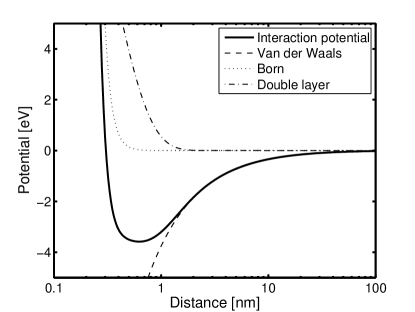
Figure 1: Interaction potential between two equal spherical particles of radius $a=0.735~{}\mathrm{\mu m}$. The potential comprises attractive Van der Waals interactions with a Hamaker constant of $A=0.062~{}{\rm eV}$, repulsive electrostatic interactions in an $150~{}\mathrm{mM}$ $\mathrm{MgCl_{2}}$ aqueous solution, a surface potential of $\phi_{0}=40\text{mV}$ and the Born repulsion where $N$ is assumed to be $N=10^{-23}$

IV Novel Tangential force model

IV.1 The model

There is quite a number of tangential force models available for DEM simulations. For example the models by Haff and Werner Haff and Werner (1986), Walton and Brown Walton and Braun (1986) or Cundall and Strack Cundall and Strack (1979). For some detail on these models the reader is referred to Kruggel-Emden et al. (2008). For this work the main deficiency of all these models is that most of them are not capable of supporting bending moments between bonded particles, except the ones which will be discussed and compared to our model in section IV.3. In the following we propose a novel tangential force model, similar to that by Cundall and Strack, which can reproduce the phenomena described in section II. In the Cundall-Strack model a spring $\boldsymbol{\xi}_{ij}$ with rigidity $k_{t}$ will be initialized when two particles, $i$ and $j$, get into contact. This spring grows proportional to the relative tangential velocity at the contact point:

$$\boldsymbol{\xi}(t)=\int_{t_{0}}^{t}dt^{\prime}\boldsymbol{v}_{t}(t^{\prime})\quad\Rightarrow\quad\dot{\boldsymbol{\xi}}=\boldsymbol{v}_{t}.$$ (8)

Here $t_{0}$ is the time when the particles get into contact. The relative tangential velocity is given by

$$\boldsymbol{v}_{t}=(\boldsymbol{v}_{j}-\boldsymbol{v}_{i})_{t}+a\left(\boldsymbol{\omega_{j}}+\boldsymbol{\omega_{i}}\right)\times\boldsymbol{n}_{ij}~{},$$ (9)

where $\boldsymbol{n}_{ij}$ is defined as $(\boldsymbol{r}_{j}-\boldsymbol{r}_{i})/|\boldsymbol{r}_{j}-\boldsymbol{r}_{i}|$. The subscript $t$ denotes the projection of the relative velocity onto the tangential plane. If the force due to the tangential spring exceeds an upper bound, which in the work by Cundall and Strack Cundall and Strack (1979) is the Coulomb friction $\mu F_{n}$, the spring will be set to

$$\boldsymbol{\xi}=\mu\frac{F_{n}}{k_{t}}\frac{\boldsymbol{\xi}}{|\boldsymbol{\xi}|}~{},$$ (10)

where $\mu$ is the friction coefficient. To make sure that the tangential force acts only in tangential direction, the Cundall-Strack spring is mapped to the tangential plane perpendicular to $\boldsymbol{n}_{ij}$ after each time-step. The tangential forces and torques acting on the $i$’th and the $j$’th particle are given by

$$\boldsymbol{F}_{t,i} =k_{t}\boldsymbol{\xi} \boldsymbol{M}_{i} =\hskip 7.11317ptR_{i}\boldsymbol{F}_{t,i}\times\boldsymbol{n}_{ij}$$ (11)

$$\boldsymbol{F}_{t,j} =-k_{t}\boldsymbol{\xi} \boldsymbol{M}_{j} =-R_{j}\boldsymbol{F}_{t,j}\times\boldsymbol{n}_{ij}$$ (12)

This model is able to capture a lot of phenomena like sliding friction and sticking friction. However, it is not able to support a bending moment between two bonded particles, which becomes obvious by the following example. We assume a fixed (no translation or rotation) particle bonded to a second particle as sketched in figure 2. An external force perpendicular to the center-center line of the particles acts on the second particle. Now we look for a static solution of the evolution equations, in which all resulting forces and moments have vanished. From equations (11) and (12) immediately follows that this is only the case if $\boldsymbol{\xi}=0$. This in turn means that the whole external force must be equilibrated by the normal forces between the particles and this can only be the case if the center-center line is finally parallel to the direction of the external force. However, this means that the bond cannot support any bending moment.

Figure 2: Example for the bending torque, the lower particle is fixed and on the upper particle acts a tangential force (left side). If the bond between the particles is able to support a bending moment, a stationary angel $\phi<\pi/2$ between the original contact line and the stationary contact line should be reached.

In order to derive a similarly simple model, however capable of supporting bending moments, we use the following reasoning: When two particles get in contact, we introduce two thought rods rigidly connected to one particles center and reaching to the center of the other particle as sketched in figure 3. Between the end point of the rod and the center of the other particle a spring will be initialized. This spring grows proportional to the relative tangential velocity between the rods end points and the particle center. The evolution equations for the springs are then

Figure 3: Sketch of tangential force model. (a) When two particles get in contact two thought rods are initialized. The rods are rigidly connected to the center of one particle and reach the other particles center. (b) According to the tangential movement of the particles the springs $\boldsymbol{\xi}_{ij}$ and $\boldsymbol{\xi}_{ji}$ will elongated. The arrows denote the direction of the vectors $\boldsymbol{\xi}_{ij}$ and $\boldsymbol{\xi}_{ji}$

$$\dot{\boldsymbol{\xi}}_{ij} =(\boldsymbol{v}_{j}-\boldsymbol{v}_{i})_{t}-\left(\boldsymbol{\omega_{i}}\times\boldsymbol{n}_{ij}\right)2a~{},$$ (13)

$$\dot{\boldsymbol{\xi}}_{ji} =(\boldsymbol{v}_{i}-\boldsymbol{v}_{j})_{t}+\left(\boldsymbol{\omega_{j}}\times\boldsymbol{n}_{ij}\right)2a~{},$$ (14)

where $\boldsymbol{\xi}_{ij}$, $\boldsymbol{\xi}_{ji}$ are defined in figure 3. The forces and moments acting on the particles are therefore

$$\boldsymbol{F}_{i} =k_{t}\left(\boldsymbol{\xi}_{ij}-\boldsymbol{\xi}_{ji}\right)~{}, \boldsymbol{M}_{i} =2ak_{t}\boldsymbol{n}_{ij}\times\boldsymbol{\xi}_{ij}~{},$$ (15)

$$\boldsymbol{F}_{j} =k_{t}\left(\boldsymbol{\xi}_{ji}-\boldsymbol{\xi}_{ij}\right)~{}, \boldsymbol{M}_{j} =-2ak_{t}\boldsymbol{n}_{ij}\times\boldsymbol{\xi}_{ji}~{}.$$ (16)

Equivalent to the Cundall-Strack model both tangential springs are mapped to the plane perpendicular to $\boldsymbol{n}_{ij}$ after each time step. The springs stop extending if its elongation exceeds a maximum value $\xi_{\rm max}$. Unlike the model of Cundall and Strack, this model is able to support bending moments. Let us demonstrate that by the same example as above.

By solving the steady state equations one find in the case of small deflections for the reorientation angle $\phi$:

$$\phi=\frac{F_{\rm Bend}}{k_{t}2a}~{}.$$ (17)

Note that our model has some similarity to a theoretical approach introduced in Zaccone et al. (2007) where a random network of springs (normal and tangential) was used to predict the elastic moduli for disordered packings of interconnected spheres. Here the tangential spring stiffness was determined by the predictive model of Pantina and Furst Pantina and Furst (2005, 2006).

We assume the model to be valid also for non-tenuous aggregates as long as pairwise contact forces can be assumed. In this contribuition we content ourselves with polymeric primary particles as investigated in Pantina and Furst (2005). Whether our model is also applicable to other types of particles (e.g. inorganic and surfactant-coated colloids) can not be revealed by the model itself but has to be clarified experimentally.

IV.2 Parameter determination

The introduced model contains two parameters. The spring stiffness $k_{t}$ and the maximum spring length $\xi_{\rm max}$. Both parameters can be determined by the experiments presented in Pantina and Furst (2005). As shown in appendix B the static shape of a linear chain of particles under a bending stress is given in leading order approximation by

$$\frac{y(x)}{F_{\rm Bend}}=-\frac{1}{8a^{3}k_{t}}\left(\frac{L}{4}x^{2}-\frac{|x|^{3}}{6}\right)~{},$$ (18)

where $L$ is the center-center distance of the first and the last particle in the chain. By comparison with equation (1) one finds

$$EI=8a^{3}k_{t}~{}.$$ (19)

From the elongation of the chain, $\delta=y(0)-y(L/2)$, one finds by comparison with equation (2) $\kappa=192(a/L)^{3}k_{t}$ and therefore from (3):

$$k_{t}=\frac{\kappa_{0}}{192}~{}.$$ (20)

Using equation (20) one directly obtains the model parameter for the tangential stiffness $k_{t}$ from the measured value $\kappa_{0}$. The value of $\xi_{\rm max}$ can be obtained from the measurement of the critical bending moment $M_{c}$ in Pantina and Furst (2005). The bending torque acting on a particle is given by equation (15) or (16). Since $\boldsymbol{n}_{ij}$ and $\boldsymbol{\xi}_{ij}$ are perpendicular to each other $\xi_{\rm max}$ has to be

$$\xi_{\rm max}=\frac{M_{c}}{2ak_{t}}~{}.$$ (21)

Thus, all parameters of the force model can be determined from experimental data. Alternatively, the predictive formulas derived by Pantina and Furst Pantina and Furst (2005, 2006) for the single bend rigidity $\kappa_{0}$ may be used to estimate the model parameters.

IV.3 Comparison to other models

In Potanin (1993) a model derived by Kantor and Webman Kantor and Webman (1984) was applied to computer simulations of two dimensional colloidal aggregates in shear flows. That model assumes that the contribution of tangential deformation to the strain energy is proportianal to

$$E\propto\sum_{i,j,k}\delta\Phi_{ijk}^{2}~{},$$ (22)

where $\delta\Phi_{ijk}$ is the change in the angle between the bonds $(i,j)$ and $(i,k)$ connected to particle $i$. The contribution to the interaction force can be described by

$$\boldsymbol{F}_{ij}=-\beta\sum_{k}\delta\Phi_{ijk}\boldsymbol{n}_{ik}\cdot(\boldsymbol{n}_{ij}\cdot\boldsymbol{n}_{ik})~{}.$$ (23)

It is mentioned in Potanin (1993) that a chain of particles connected by such forces behaves like a thin elastic rod with the same length. As shown in appendix A, our model leads in the case of a linear structure (i. e. every particle is bonded to a maximum of two other particles) to an elastic equilibrium energy of

$$E=a^{2}k_{t}\sum_{i}\delta\Phi_{i}~{},$$ (24)

where $\delta\Phi_{i}$ denotes the change of the angle between the two bonds ending on particle $i$. Due to the fact that (24) and (22) are equivalent, the equilibrium elastic deformation of our model is also equivalent.

The main difference between the two models is that our model takes only pairwise interactions into account, while the model by Kantor and Webman Kantor and Webman (1984) is a three particle interaction model. The tangential forces and the bending energy are there related to the change of angles between neighboring bonds. However, one would expect that the energy is stored directly in the bonds. It remains unclear why the angle between two different bonds is the measure for the elastic energy. Although the same behavior is observed in our proposed model, the reason is quite obvious. The energy is directly stored in the bonds but neighboring bonds are related due to the equilibrium conditions. In contrast to the model of Kantor and Webman the proposed model is suited to describe non-elastic displacements of the bonds, which occur if the maximum supported bending moment is reached. Furthermore, the tracking of angles between all bonds ending on the same particle may cause much higher implementatory (and possibly computational) effort compared to the proposed model.

To avoiding the computational problems caused by tracking of the angles, West, Melrose and Ball West et al. (1994) proposed a model where the basic colloidal unit is replaced by a trimer of stiff spheres and the interactions are assumed as superposition of $3\times 3$ pairwise interacting central forces. Depending on the relative orientation of the trimers, bonds between two trimers are able to support bonding moments. Contrary to our proposed model this only provides qualitative information. Besides, no relation between experimental data and model parameters is available. Furthermore replacing one particle by three particles leads to a higher computational effort. Nevertheless, the ansatz of West, Melrose and Ball is probably superior to our model for the simulation of colloids containing non-spherical primary particles.

The model of of Botet and Cabane Botet and B. (2004) is in principle able to capture the effect observed by Pantina and Furst Pantina and Furst (2005). They modeled the interactions between two spheres by a number of springs connected to pins which are randomly distributed over the spheres. In comparison to our model the model of Botet and Cabane Botet and B. (2004) consumes much more computational resources in order to handle the pins and springs. Furthermore, the estimation of the model parameters, i. e. number of pins, spring stiffness, equilibrium and breakage lengths, seemed to be more difficult.

V Simulation method and results

We assume spherical mono-disperse colloidal particles immersed in an aqueous ${\rm MgCl_{2}}$ solution. Unless otherwise noted we used the parameters from Pantina and Furst (2005). The radius of the particles is $a=0.735~{}{\rm\mu m}$. The surface potential is $\phi_{0}=40~{}{\rm mV}$. We use the Discrete Element Method Cundall and Strack (1979); Poeschel and Schwager (2005) to simulate aggregate structure evolution. The main idea of this method is to track the trajectories of all primary particles by solving Newton’s equations of motion numerically. In general the state of the particle system is given by the particle positions $\left\{\boldsymbol{r}_{1},\boldsymbol{r}_{2}...\boldsymbol{r}_{N}\right\}$, velocities $\left\{\boldsymbol{v}_{1},\boldsymbol{v}_{2},...,\boldsymbol{v}_{n}\right\}$ and by the angular velocities $\left\{\boldsymbol{\omega}_{1},\boldsymbol{\omega}_{2},..\boldsymbol{\omega_{n}}\right\}$. Note that there is no need to track the particles’ orientation angles as we content ourselves with spherical particles. For the interactions between the fluid and the particles we use the free draining approximation: Every particle experiences the unperturbated flow field as if no other particle were in the flow. The drag force and torque acting on the $i$’th particle is then given by Stokes formulas: Landau and Lifschitz (1993)

$$\boldsymbol{F}_{{\rm drag},i} =6\pi\eta a(\boldsymbol{v}_{i}-\boldsymbol{u}(\boldsymbol{r}_{i}))\,,$$ (25)

$$\boldsymbol{M}_{{\rm drag},i} =8\pi\eta a^{3}(\boldsymbol{\omega}_{i}-\boldsymbol{\Omega}(\boldsymbol{r}_{i}))~{}.$$ (26)

With $\eta$, $\boldsymbol{v}_{i}$, and $\boldsymbol{u}(\boldsymbol{r}_{i})$ being the dynamic viscosity of the carrier fluid, the velocity of $i$’th particle and the fluid velocity at the position of $i$’th particle, respectively. $\Omega=1/2\nabla\times\boldsymbol{u}$ is the vorticity of the fluid velocity field. For the considered particles, effects of inertia can surely be neglected. Therefore, the particle dynamic is governed by the overdampded equations of motion:

$$\dot{\boldsymbol{r}}_{i} =\frac{1}{6\pi\eta a}\boldsymbol{F}_{i}+\boldsymbol{u}(\boldsymbol{r}_{i})~{},$$ (27)

$$\boldsymbol{\omega}_{i} =\frac{1}{8\eta\pi a^{3}}\boldsymbol{M}_{i}+\Omega(\boldsymbol{r}_{i})~{}.$$ (28)

The forces $\boldsymbol{F}_{i}$ and the torques $\boldsymbol{M}_{i}$ include all interaction effects acting on the $i$’th particle. For solving the equations of motion we use Heun’s method, which has a global error of order $\Delta t^{2}$ and is similar to the velocity-Verlet method, often used in molecular dynamics and DEM simulations Frenkel and Smit (2002). Note that the velocity-Verlet method itself is explicitly designed for solving Newton’s equations of motion and cannot be used in overdamped dynamics. In principle, we can use the force models described above to simulate the colloid. However, from the slope of the potential plot (figure 1) a computational problem becomes apparent. In the neighborhood of the potential minimum the interaction forces change rapidly on very small length scales. Therefore it is necessary to solve the equations of motion with very small time steps to track the details of motion and avoid instabilities of the numerical solution. We found that the magnitude of time-steps must approximately be $10^{-9}~{}{\rm s}$ to track particle motion correctly. However, if two particles are bonded to each other, the center-center distance remains approximately constant and only the angular orientation of the particles can change significantly. In order to avoid the need of such small time-steps we introduce a constraint if the distance between two particles $i$ and $j$ becomes smaller than a critical distance $d_{c}$. The equations of motion are then solved with the constraint $|\boldsymbol{r_{i}}-\boldsymbol{r_{j}}|=d_{c}$. For solving the constrained equations of motion, we adopted the RATTLE algorithm derived by Andersen Andersen (1983), which fulfills the constraint up to a given tolerance $tol$, to Heun‘s method. In this paper we used $d_{c}=1.1~{}{\rm nm}$ and $tol=0.1~{}{\rm nm}$. By careful investigation of numerical results we found that the value of $d_{c}$ has a negligible effect on the results to be presented below as long as $d_{c}$ is much smaller than the primary particles’ diameter $a$. With the chosen parameters we were able to use time-steps of the order of $10^{-6}~{}{\rm s}$, which leads to remarkable improvements in simulation time. However, the time needed by the Anderson algorithm is proportional to the number of bonds in the aggregate and especially for large compact structures the computation time may grow fast with the number of particles used in the simulation.

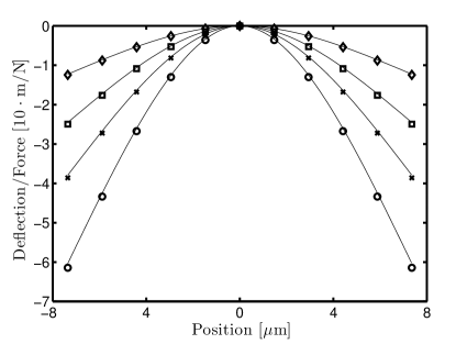
Figure 4: Simulated shape of a bended 11-particle aggregate for different material parameters. The used tangential stiffness are $k_{t}=0.785~{}{\rm mN/m}$ (circles), $k_{t}=1.1~{}{\rm mN/m}$ (crosses), $k_{t}=1.7~{}{\rm mN/m}$ (squares) and $k_{t}=3.4~{}{\rm mN/m}$ (diamonds). The Symbols are simulation results and the lines are obtained from (1).

In order to reproduce the results of Pantina and Furst, we performed simulations where a linear chain of particles is bended. We applied an external force $F_{\rm Bend}$ directed perpendicular to the chain of particles to the middle particle. We compensate this force by applying $-F_{\rm Bend}/2$ on the terminal particles of the chain. Then we run the simulation until the static shape is achieved. Note that the value of the fluid viscosity has no influence on the static solution, but only on the time needed to achieve it. Figure 4 shows simulated deflection curves for an aggregate comprising $11$ particles for different spring stiffness $k_{t}=0.69;~{}1.1;~{}1.7;~{}3.4~{}{\rm mN/m}$. These values correspond to the measured $\kappa_{0}$ for different ${\rm MgCl_{2}}$ concentrations ($150;~{}250;~{}375;~{}500~{}\rm{mM}$, respectively Pantina and Furst (2005). All four curves are well described by equation (1) (solid lines) with $EI$ obtained from equation (20).

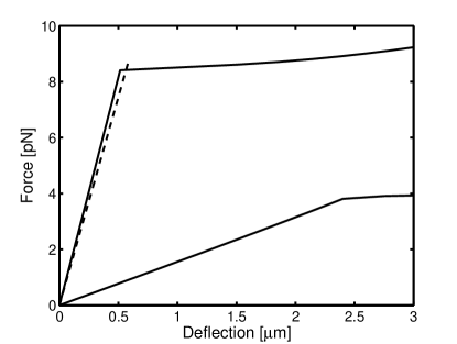
Figure 5: Typical deflection-force curves for a $11$ particle (upper line) and a 23 particle aggregate (lower curve). The parameters for the tangential force model are $k=0.69~{}{\rm mN/m}$ and $\xi_{\rm max}=30.48~{}{\rm nm}$ obtained from measured data in Pantina and Furst (2005) for a 150 ${\rm MgCl_{2}}$ solution. The dashed line shows the experimentally obtained linear part of deflection-force curve taken from a data plot (figure 2) presented by Pantina and Furst (2005).

Figure 5 shows typical deflection vs. force curves. Here the measured value of $\kappa_{0}=0.13~{}\rm{N/m}$ for a 150 mM ${\rm MgCl_{2}}$ concentration was used Pantina and Furst (2005). For small deflections, the aggregate is bended similar to a rigid rod as described above. In that regime the deflection vs. force curve shows a linear behavior. If the bending force exceeds a critical value, rearrangement of the particles occurs. Beyond this point, the particles form a near triangular structure. The simulation results in the linear regime and the critical force where the rearrangement occurs are in agreement with the experimental data presented in Pantina and Furst (2005) figure 2. Note that for experimental reasons the relevant part of the data presented by Pantina and Furst (2005) are on a deflection interval of approx. $1.5-2~{}{\rm\mu m}$. The reason is some tortouisity in the chains, which must be unbend before the linear elongation regime starts . The simulated behavior after reaching rearrangement is different from the experimental data. This is due to the fact that the terminal particles in the experiment are trapped by optical tweezers while in the simulation only a force perpendicular to the linear chain direction is applied. The behavior of both setups is comparable as long as particles’ displacements in $x$ direction are small. However, this is no longer the case if the rearrangement to triangular structures has occurred.

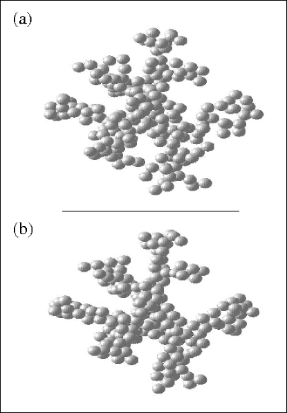
Figure 6: Compaction of an aggregate using central forces only. (a) The start configuration, generated by diffusion limited aggregation. (b) The configuration after a simulated time period of 25s, the structure is significantly more compact than the starting configuration.

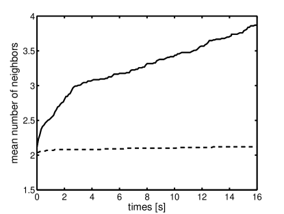
Figure 7: Time evolution of the average number of neighbors. The solid line shows simulation results where DLVO forces only were considered. The dashed line displays data obtained from simulations where the tangential force model was applied.

Finally, we used our simulation to track the time evolution of an aggregate comprising 200 primary particles in a resting fluid. The initial aggregate was obtained by diffusion-limited cluster particle aggregation Witten and Sander (1983). We compared the results by using the classical DLVO forces only with the results obtained using our tangential force model. Figure 6 shows the initial aggregate and the restructured aggregate after 25 seconds using DLVO forces only. It is remarkable that even in a resting fluid the aggregate collapses to more a compact structure. This behavior obviously is a result of the used force models. The van der Waals forces act over a relatively long range. As there is no resistance of single particle bonds against bending moments, the bonded particles can freely reorient. This behavior contradicts the observation that fractal structure are often stable over long times even in moderate shear flows Selomulya et al. (2001, 2002). This indicates that assuming purely central forces is an over-simplification which hinders prediction of realistic structure evolution. Under the same conditions, but using the introduced tangential force model, the compaction does not occur. In order to quantify the compaction of the aggregate we count the number of neighboring particles for each particle. The average number of neighbors is used as a measure for the compactness. Particles are considered to be neighbors if their surface-surface distance is below $10~{}$nm. Note that we deliberately do not use the fractal dimension as a measure for compactness because the aggregate looses the property of self-similarity during the compaction process. Figure 7 shows the time evolution of the average number of neighbors for the case of using DLVO forces only and for the case of using DLVO augmented with our tangential model. In case of using DLVO only, the number of neighbors grows continuously, while the compaction of the aggregate is negligible if the tangential model is used.

VI Summary and Conclusion

In this work we have introduced a new model for tangential interaction forces applicable in computer simulations. Our tangential force model is capable of supporting bending moments. This is an important quality as it has been recently shown experimentally that colloidal bonds actually support bending moments Pantina and Furst (2005). Our model is based on two tangential springs acting between bonded particles. The time evolution of these springs is determined by the relative tangential velocity between the particles. The spring elongation is constrained to a maximum elongation to account for sliding effects. The model contains two parameters: The stiffness of the springs and the maximum elongation. We showed that both parameters can be determined directly from the experiments shown in Pantina and Furst (2005) and simulations using our model are able to reproduce the experimental observations. We compared our model to former models which were used in computer simulations and are capable of supporting bending moments. Furthermore, we showed that even in the case of simulating a fractal aggregate in a resting fluid models without tangential forces lead to an unrealistic collapse of the aggregate. Using our tangential force model can remedy that flaw.

Appendix A Determination of the equilibrium bending energy in linear structures

Figure 8: Sketch for the calculation of the bending energy. The initial configuration is shown by solid lines. After the deformation process the three particles have new positions and orientations, shown by the dashed lines. The particles $l$ and $j$ are reoriented relative to particle $i$ by the angles $\delta\phi_{l}$ and $\delta\phi_{i}$, and particle $i$ was rotated around its center by the angle $\delta\varphi_{i}$. The springs $\xi_{i}j$ and $\xi_{i}l$ are deformed due to the particle motion.

In order to determine the bending energy in a linear structure of particles we consider three particles $l$, $i$ and $j$ of a structure which undergoes deformations as sketched in figure 8. The torque balance for particle $i$ follows from equation (15)

$$0=2ak_{t}\left(\boldsymbol{\xi}_{il}\times\boldsymbol{n}_{il}+\boldsymbol{\xi}_{ij}\times\boldsymbol{n}_{ij}\right)~{}.$$ (29)

Assuming small deformations, equation (29) can be rewritten as a scalar equation:

$$\xi_{il}-\xi_{ij}=0~{}.$$ (30)

Under the assumption that all deflections are small and no plastic deformation occurrs during deformation (i. e.  no spring length in the system exceeded $\xi_{max}$) one finds from equation (13):

$$\xi_{il}=2a\left(\delta\phi_{l}-\delta\varphi_{i}\right)~{},$$ (31)

$$\xi_{ij}=2a\left(\delta\phi_{j}+\delta\varphi_{i}\right).$$ (32)

Introducing this in equation (30) and solving the resulting equation for $\delta\varphi_{i}$ leads to

$$\delta\varphi_{i}=\frac{1}{2}(\delta\phi_{l}-\delta\phi_{j})~{}.$$ (33)

The energy stored in the springs $\xi_{il}$ and $\xi_{ij}$ is given by

$$E_{i}=\frac{1}{2}k_{t}\left(\xi_{il}^{2}+\xi_{ij}^{2}\right)$$ (34)

Introducing (31) and (32) in (34) leads to the equation

$$E_{i}=2a^{2}k_{t}\left(\delta\phi_{l}^{2}+\delta\phi_{j}^{2}+2\delta\varphi_{i}(\delta\phi_{j}-\delta\phi_{l})+2\delta\varphi_{i}^{2}\right)~{}.$$ (35)

By introducing equation (33) in (35) one obtain:

$$E_{i}=a^{2}k_{t}\left(\delta\phi_{l}+\delta\phi_{j}\right)^{2}~{}.$$ (36)

This in turn can be expressed as the change of the angle between the bond of particles $l$ and $i$ and particles $i$ and $j$: $\delta\Phi=\delta\phi_{1}+\delta\phi_{2}$. Therefore we get

$$E_{i}=a^{2}k_{t}\delta\Phi^{2}~{}.$$ (37)

By adding up $E_{i}$ for all particles in the chain one gets the whole elastic energy of the structure, except the contribution from rods rigidly connected to terminal particles to a particle within the structure. Therefore $E_{i}$ can be understood as the energy per particle in an elastic deformed linear structure of colloidal particles.

Appendix B Determination of the equilibrium shape

In order to calculate the shape of a bended chain of particles as described in IV.2, we minimize the elastic energy stored in such an elastic chain. From symmetry reasons it is sufficient to consider only half of the chain. As shown in figure 9 the change in the angle of the bonds connected to $n$’th particle is denoted as $\phi_{n}$. The bending energy per particle is therefore given by (37):

$$E_{n}=a^{2}k_{t}\phi_{n}^{2}$$ (38)

The elastic energy stored in the whole chain is therefore

$$E=2\sum_{i=1}^{N-1}a^{2}k_{t}\phi_{n}^{2}~{},$$ (39)

where $N$ is the number of particles in the half of the chain.

Figure 9: Sketch for the calculation of the equilibrium shape

In equilibrium this energy should be minimal. The position of the $n$’th particle is

$$y_{n}=-2a\sum_{i=1}^{n}\sin\left(\sum_{j=1}^{i}\phi_{j}\right)~{}.$$ (40)

Assuming small total deflection this reduces to

$$y_{n}=-2a\sum_{i=1}^{n}\sum_{j=1}^{i}\phi_{j}~{}.$$ (41)

Assuming that the total deflection of the rod is $\Delta s$ we have a constraint for the energy minimization:

$$\Delta s=2a\sum_{i=1}^{N-1}\sum_{j=1}^{i}\phi_{j}$$ (42)

Using the technique of Lagrangian multiplier we have to minimize the quantity.

$$E=\sum_{i=1}^{N-1}2a^{2}k_{t}\phi_{n}^{2}-\lambda\left(2a\sum_{i=1}^{N-1}\sum_{j=1}^{i}\phi_{j}+\Delta s\right)$$ (43)

where $\lambda$ is the Lagrangian multiplier. To minimize $E$ one has to solve

$$0=\frac{dE}{d\phi_{m}}=4a^{2}k_{t}\phi_{m}-2\lambda a\sum_{i=1}^{N-1}\sum_{j=1}^{i}\delta_{j,m}~{},$$ (44)

where $\delta_{j,m}$ is the Kronecker symbol which is equal to one if $j=m$ and zero elsewhere. The solution of this equation is

$$\phi_{m}=\frac{\lambda(N-m)}{2ak_{t}}~{}.$$ (45)

Introducing this in the constraint (42) one finds after some algebra

$$\frac{\lambda}{k_{t}}\left(\frac{1}{3}N^{3}-\frac{1}{2}N^{2}+\frac{1}{6}N\right)=\Delta s~{}.$$ (46)

Under neglecting all powers of N smaller then three one finds

$$\lambda=\frac{3k_{t}\Delta s}{N^{3}}~{},$$ (47)

and by introducing that in equation (45)

$$\phi_{m}=\frac{3}{2}\frac{\Delta s}{aN^{3}}(N-m)~{}.$$ (48)

Introducing this in equation (41), using $N=L/4a$, $m=x_{m}/a$ and neglecting all terms that vanish for $a\rightarrow 0$ one finds

$$y_{m}=\frac{\Delta s}{L^{3}}\left(6x_{m}^{2}-4|x_{m}|^{3}\right)$$ (49)

Introducing (45) in (39) results in an expression for the elastic energy as function of $N$ or $L$, respectively, and $\Delta s$. The bending force is related to that energy by

$$F_{\rm Bend}=\frac{dE}{d\Delta s}~{}.$$ (50)

Now one can eliminate $\Delta s$. After introducing $\Delta s$ in (49) the elongation is found:

$$y_{m}=\frac{F_{\rm Bend}}{8a^{3}k}\left(\frac{L}{4}x_{m}^{2}-\frac{1}{6}|x_{m}|^{3}\right)~{}.$$ (51)

References

- Doi and Chen (1989) M. Doi and D. Chen, J. Chem. Phys. 90, 5271 (1989).
- Chen and Doi (1989) D. Chen and M. Doi, J. Chem. Phys. 91, 2656 (1989).
- Higashitani et al. (2001) K. Higashitani, K. Iimura, and H. Sanda, Chem. Eng. Sci. 56, 2927 (2001).
- Hunter (1995) J. R. Hunter, Foundations of Colloid Science (Oxford Science Publications, 1995), 5th ed.
- Cundall and Strack (1979) P. A. Cundall and O. D. L. Strack, Geotechnique 29, 47 (1979).
- Poeschel and Schwager (2005) P. Poeschel and T. Schwager, Computational Granular Dynamics: Models and Algorithms (Springer, Berlin;, 2005), 2nd ed.
- Fanelli et al. (2006a) M. Fanelli, D. L. Feke, and I. Manas-Zloczower, Chem. Eng. Sci. 61, 4944 (2006a).
- Fanelli et al. (2006b) M. Fanelli, D. L. Feke, and I. Manas-Zloczower, Chem. Eng. Sci. 61, 473 (2006b).
- Harada et al. (2007) S. Harada, R. Tanaka, H. Nogmi, M. Sawada, and K. Asakura, Colloids Surfaces A Physicochem. Eng. Aspects 302, 396 (2007).
- Durlofsky et al. (1987) L. Durlofsky, J. F. Brady, and G. Bossis, J. Fluid Mech. 180, 21 (1987).
- Brady and Bossis (1988) J. F. Brady and G. Bossis, Annu. Rev. Fluid Mech. 20, 111 (1988).
- Feng et al. (1984) S. Feng, P. N. Sen, B. I. Halperin, and C. J. Lobb, Phys. Rev. B 30, 5386 (1984).
- Feng and Sen (1984) S. Feng and P. N. Sen, Phys. Rev. Lett. 52, 216 (1984).
- Kantor and Webman (1984) Y. Kantor and I. Webman, Phys. Rev. Lett. 52, 1891 (1984).
- Schwartz et al. (1985) L. M. Schwartz, S. Feng, M. F. Thorpe, and P. N. Sen, Phys. Rev. B 32, 4607 (1985).
- Potanin (1992) A. A. Potanin, J. Chem. Phys. 96, 9191 (1992).
- Born (1954) M. Born, K. Huang, Dynamical Theory of Crystal Lattices (Oxford University, New York, 1954).
- Potanin (1993) A. A. Potanin, J. Colloid Interface Sci. 157, 399 (1993).
- West et al. (1994) A. H. L. West, J. R. Melrose, and R. C. Ball, Phys. Rev. E 49, 4237 (1994).
- Botet and B. (2004) R. Botet and B. Cabane, Phys. Rev. E 70, 031403 (2004).
- Pantina and Furst (2005) J. P. Pantina and E. M. Furst, Phys. Rev. Lett. 94, 138301 (2005).
- Pantina and Furst (2006) J. P. Pantina and E. M. Furst, Langmuir 22, 5282 (2006).
- Israelachvili (1994) J. Israelachvili, Intermolecular & Surface Forces (Academic Press Limited, 1994), 2nd ed.
- Feke et al. (1984) D. L. Feke, N. D. Prabhu, and J. A. Mann, J. Chem. Phys. 88, 5735 (1984).
- Haff and Werner (1986) P. K. Haff and B. T. Werner, Powder Technology 48, 239 (1986).
- Walton and Braun (1986) O. R. Walton and R. L. Braun, Journal Of Rheology 30, 949 (1986).
- Kruggel-Emden et al. (2008) H. Kruggel-Emden, S. Wirtz, and V. Scherer, Chem. Eng. Sci. 63, 1523 (2008).
- Zaccone et al. (2007) A. Zaccone, M. Lattuada, H. Wu, and M. Morbidelli, J. Chem. Phys. 127, 174512 (2007).
- Landau and Lifschitz (1993) L. D. Landau and E. M. Lifschitz, Lehrbuch der theoretischen Physic, Band VI Hydrodymik (Akademie Verlag Gmbh, 1993), 5th ed.
- Frenkel and Smit (2002) D. Frenkel and B. J. Smit, Understanding Molecular Simulation (Academic Press, 2002).
- Andersen (1983) H. C. Andersen, J. Comput. Phys. 52, 24 (1983).
- Witten and Sander (1983) T. A. Witten and L. M. Sander, Phys. Rev. B 27, 5686 (1983).
- Selomulya et al. (2001) C. Selomulya, R. Amal, G. Bushell, and T. D. Waite, J. Colloid Interface Sci. 236, 67 (2001).
- Selomulya et al. (2002) C. Selomulya, G. Bushell, R. Amal, and T. D. Waite, Langmuir 18, 1974 (2002).