The Photometric Variability of HH 30

Abstract

HH 30 is an edge-on disk around a young stellar object. Previous imaging with the Hubble Space Telescope has show morphological variability that is possibly related to the rotation of the star or the disk. We report the results of two terrestrial observing campaigns to monitor the integrated magnitude of HH 30. We use the Lomb-Scargle periodogram to look for periodic modulation with periods between 2 days and almost 90 days in these two data sets and in a third, previously published, data set. We develop a method to deal with short-term correlations in the data. Our results indicate that none of the data sets shows evidence for significant periodic photometric modulation.

HH 30 es un disco visto casi de canto alrededor de un objeto estelar joven. Imágenes previas del Hubble Space Telescope muestran una variabilidad morfológica que posiblemente esté relacionada con la rotación de la estrella o el disco. Reportamos los resultados de dos campañas observacionales realizadas con un telescopio terrestre para monitorear la magnitud integrada de HH 30. Usamos el periodograma de Lomb-Scargle para buscar modulaciones periódicas con periodos entre 2 y casi 90 días en estos dos conjuntos de datos y en un tercer conjunto de datos previamente publicado. Desarrollamos un método para mitigar los efectos de las correlaciones de periodo corto en los datos. Nuestros resultados indican que ninguno de los conjuntos de datos muestra evidencia de una modulación periódica en su photometría.

accretion, accretion disks circumstellar matter stars: individual (HH 30) stars: pre-main sequence

0.1 Introduction

High-resolution images show that HH 30 is a compact bipolar reflection nebula bisected by a dark lane (Burrows et al. 1996). Its location in the L1551 molecular cloud and similarity to the model images of Whitney & Hartman (1992) led immediately to the conclusion that HH 30 is an optically-thick circumstellar disk seen almost edge-on around a young stellar object.

An interesting aspect of HH 30 is the prominent morphological variability (Burrows et al. 1996; Stapelfeldt et al. 1999; Cotera et al. 2001; Watson & Stapelfeldt 2007). This variability includes changes in the contrast between the brighter and fainter nebulae over a range of more than one magnitude; changes in the lateral contrast between the two sides of the brighter nebula over a range of more than one magnitude; and changes in the lateral contrast between the two sides of the fainter nebula over a range of about half a magnitude. It appears that the central source is acting as a lighthouse, preferentially illuminating different parts of the disk.

Two mechanisms have been suggested for the lighthouse. Wood & Whitney (1998) suggested non-axisymmetric stellar accretion hot-spots. Stapelfeldt et al. (1999) suggested voids or clumps in the inner disk. AA Tau seems to be a prototype for both mechanisms, apparently possessing both inclined hot spots and occulting inner-disk warps, both presumably the result of an inclined stellar magnetic dipole (Bouvier et al. 1999; Ménard et al. 2003; O’Sullivan et al. 2005).

The two mechanisms are likely to be periodic, as they are expected to be tied to stellar rotation and orbital motions. Therefore, there is a hope that we might see a periodic modulation in the integrated photometry of HH 30, as one might expect the nebulae to be observed to be brighter when the lighthouse beam is pointing towards the observer. In this work we report an unsuccessful attempt to detect such a periodic modulation in three data sets.

0.2 Observations

0.2.1 Data Set 1

We observed HH 30 with the 84 centimeter telescope of the Observatorio Astronómico Nacional on Sierra San Pedro Mártir on 24 of the 28 nights between 1999 January 29 and 1999 February 25. We used the SITe1 $1024\times 1024$ CCD binned $1\times 1$ with the observatory’s $R$ (2 mm KG3 and 2 mm OG570) and $I$ (4 mm RG9) filters.

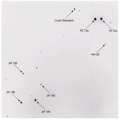
Figure 1: An image of the field of HH 30 in $I$ taken on 1999 January 29. North is approximately up and east is approximately left. The image is approximately $7^{\prime}$ to a side. This pointing is typical of those used to obtain data set 1. The local standard is 2MASS 04314544+1814359, which does not vary significantly with respect to the stars JH 192, 193, 194, and 195.

We selected the pointing to include both HH 30 and several stars to the south-east. A typical pointing is shown in Figure 1. We used roughly the same pointing each night, to minimize variations in residual flat field error. Each night we typically took two consecutive 600 second exposures in $R$ and two consecutive 300 second exposures in $I$, although on the night of 1999 February 11 we were able to observe only in $R$. The image quality was typically $2^{\prime\prime}$ FWHM, and we often observed through clouds.

We reduced each image by subtracting an offset calculated from the overscan, subtracting a residual bias image, and dividing by a twilight-sky flat field. We obtained instrumental magnitudes of all of the bright sources in the field using aperture photometry with an object aperture of diameter $8^{\prime\prime}$ and a sky annulus with an inner diameter of $8^{\prime\prime}$ and an outer diameter of $16^{\prime\prime}$. We averaged the instrumental magnitudes in the consecutive images in each filter.

8 $\Delta R$ $\Delta I$ JH 2MASS $\bar{m}$ $\sigma_{m}$ $\bar{m}$ $\sigma_{m}$ JH 192 J04315455+1809573 $+1.002$ 0.013 $+0.534$ 0.018 JH 193 J04315915+1810391 $+0.473$ 0.015 $-0.033$ 0.019 JH 194 J04315607+1808595 $-1.483$ 0.009 $-1.466$ 0.017 JH 195 J04315981+1808517 $-0.779$ 0.013 $-1.335$ 0.016

Table 1: Stability of the Local Standard in 1999 January and February

We adopted the star 2MASS 04314544+1814359 as a local standard. This star lies $131^{\prime\prime}$ north and $114^{\prime\prime}$ east of HH 30 and is marked in Figure 1. Table 1 shows differential photometry of stars JH 192, 193, 194, and 195 (Jones & Herbig 1979 and Figure 1) against the local standard. In Table 1, $\bar{m}$ is the mean magnitude difference over the run and $\sigma_{m}$ is the empirical estimate of the standard deviation of a single magnitude difference. The standard deviations are all less than 2%, and show that the local standard did not vary significantly during the course of our observations.

9

Table 2: Data Set 1: Photometry of HH 30 from 1999 January and February

		$\Delta R$				$\Delta I$
Date		JD	$m$	$\sigma_{m}$		JD	$m$	$\sigma_{m}$
1999 Jan 29		2451208.800	1.628	0.016		2451208.788	2.184	0.014
1999 Jan 30		2451209.648	1.726	0.047		2451209.626	2.210	0.011
1999 Jan 31		2451210.627	1.639	0.012		2451210.647	2.219	0.013
1999 Feb 01		2451211.661	1.604	0.013		2451211.644	2.124	0.011
1999 Feb 02		2451212.730	1.504	0.010		2451212.750	2.071	0.012
1999 Feb 03		2451213.682	1.743	0.011		2451213.664	2.236	0.011
1999 Feb 06		2451216.642	2.081	0.011		2451216.629	2.746	0.016
1999 Feb 07		2451217.618	2.069	0.011		2451217.603	2.746	0.019
1999 Feb 09		2451219.632	2.171	0.012		2451219.620	2.898	0.019
1999 Feb 11		2451221.672	2.089	0.020
1999 Feb 12		2451222.675	2.114	0.010		2451222.659	2.710	0.015
1999 Feb 13		2451223.756	1.769	0.008		2451223.740	2.320	0.011
1999 Feb 14		2451224.686	1.702	0.007		2451224.662	2.276	0.010
1999 Feb 15		2451225.617	1.627	0.008		2451225.605	2.195	0.010
1999 Feb 16		2451226.686	1.855	0.010		2451226.662	2.442	0.013
1999 Feb 17		2451227.628	1.978	0.012		2451227.619	2.586	0.017
1999 Feb 18		2451228.633	1.946	0.012		2451228.615	2.574	0.016
1999 Feb 19		2451229.688	1.849	0.010		2451229.664	2.405	0.012
1999 Feb 20		2451230.681	1.653	0.008		2451230.665	2.166	0.010
1999 Feb 21		2451231.686	1.741	0.009		2451231.669	2.270	0.010
1999 Feb 22		2451232.667	1.777	0.034		2451232.653	2.332	0.015
1999 Feb 23		2451233.698	1.859	0.043		2451233.685	2.349	0.042
1999 Feb 24		2451234.647	1.550	0.019		2451234.631	2.088	0.024
1999 Feb 25		2451235.680	1.562	0.011		2451235.673	2.055	0.011

In Table 2 we report differential photometry of HH 30 against the local standard in the instrumental $R$ and $I$ systems. In Table 2, $m$ is the relative magnitude of HH 30 (that is, the instrumental magnitude of HH 30 minus instrumental magnitude of the local standard) and $\sigma_{m}$ is the standard deviation in each relative magnitude estimated from photon statistics. The standard deviation of a single measurement about the mean is 0.242 in $R$ and 0.199 in $I$. These are an order of magnitude larger than the variations seen in Table 1 between the local standard and four field stars and an order of magnitude larger than the expected errors from photon statistics. This suggests that the variability of HH 30 in data set 1 is real.

0.2.2 Data Set 2

13

Table 3: Data Set 2: Photometry of HH 30 from 1999 September to 2000 February

		Instrumental $V$				Instrumental $R$				Instrumental $I$
Date		JD	$m$	$\sigma_{m}$		JD	$m$	$\sigma_{m}$		JD	$m$	$\sigma_{m}$
1999 Sep 07		2451428.9921	14.207	0.027		2451428.9960	13.390	0.039		2451428.9985	13.506	0.040
		2451429.0017	14.184	0.032		2451429.0055	13.414	0.039		2451429.0080	13.520	0.040
1999 Sep 08		2451429.9946	14.107	0.040		2451429.9984	13.345	0.052		2451430.0009	13.493	0.053
						2451430.0077	13.360	0.045		2451430.0103	13.487	0.051
1999 Sep 11		2451433.0002	13.838	0.041		2451433.0041	13.236	0.040		2451433.0066	13.415	0.041
		2451433.0107	13.877	0.026		2451433.0146	13.264	0.033		2451433.0171	13.469	0.042
1999 Sep 13		2451435.0059	14.076	0.037		2451435.0098	13.376	0.049		2451435.0123	13.551	0.053
1999 Sep 14		2451435.9991	14.647	0.054		2451436.0030	13.883	0.049		2451436.0055	14.057	0.060
1999 Sep 15		2451436.9653	14.982	0.046		2451436.9692	14.042	0.049		2451436.9717	14.275	0.066
1999 Oct 07		2451459.0033	15.242	0.086		2451459.0072	14.155	0.028		2451459.0097	14.497	0.027
		2451459.0131	15.182	0.023		2451459.0170	14.205	0.026		2451459.0195	14.506	0.028
1999 Oct 08						2451460.0157	14.111	0.017		2451460.0182	14.513	0.022
1999 Oct 09		2451460.9976	15.030	0.030		2451461.0018	14.090	0.021		2451461.0044	14.446	0.016
1999 Oct 12		2451463.9639	14.355	0.020		2451463.9678	13.623	0.027		2451463.9703	13.826	0.024
		2451463.9734	14.340	0.014		2451463.9772	13.634	0.022		2451463.9797	13.814	0.024
		2451463.9829	14.361	0.016		2451463.9875	13.641	0.022		2451463.9900	13.828	0.020
1999 Oct 30		2451481.9541	14.641	0.028		2451481.9580	13.787	0.020		2451481.9605	13.976	0.018
		2451481.9663	14.625	0.037		2451481.9702	13.741	0.015		2451481.9727	14.008	0.024
		2451481.9753	14.656	0.046		2451481.9792	13.757	0.019		2451481.9817	14.001	0.017
						2451481.9881	13.771	0.019
1999 Nov 05		2451487.9283	14.980	0.058		2451487.9322	13.996	0.067		2451487.9347	14.277	0.072
1999 Dec 03		2451515.7883	14.676	0.020						2451515.7947	14.078	0.018
1999 Dec 08		2451520.7739	14.814	0.029		2451520.7778	13.991	0.029		2451520.7803	14.266	0.036
		2451520.7929	14.816	0.031		2451520.7967	14.043	0.036		2451520.7992	14.357	0.041
2000 Jan 23						2451566.6145	13.345	0.041		2451566.6167	13.627	0.041
2000 Jan 26		2451569.6053	14.014	0.041		2451569.6000	13.264	0.041		2451569.6020	13.471	0.041
2000 Jan 30		2451573.5785	14.534	0.041		2451573.5729	13.660	0.041		2451573.5754	13.782	0.041
2000 Feb 28		2451602.6122	14.899	0.020		2451602.6153	13.990	0.029		2451602.6179	14.320	0.024

Wood et al. (2000) report observations of HH 30 with Harris $VRI$ filters at the 1.2 meter telescope of the F. L. Whipple Observatory on 18 nights between 1999 September 7 and 2000 February 28. HH 30 was observed more than once on 7 of these nights. These authors kindly made available their reduced photometry, and we reproduce it in Table 3 for posterity. The magnitudes in Table 3 are instrumental magnitudes. The standard deviation of a single measurement about the mean is 0.408 in $V$, 0.315 in $R$, and 0.378 in $I$.

0.2.3 Data Set 3

13

Table 4: Data Set 3: Photometry of HH 30 from 2005 September to 2006 February

		$I$
Date		JD	$m$	$\sigma_{m}$
2005 Sep 11		2453624.97	16.86	0.05
2005 Sep 13		2453626.95	17.53	0.05
2005 Sep 15		2453628.95	17.25	0.05
2005 Sep 16		2453629.93	16.86	0.05
2005 Sep 17		2453630.95	16.85	0.05
2005 Sep 18		2453631.94	17.10	0.05
2005 Sep 19		2453632.93	17.16	0.05
2005 Sep 25		2453638.94	16.48	0.05
2005 Sep 26		2453639.94	16.73	0.05
2005 Oct 22		2453665.87	17.71	0.05
2005 Oct 23		2453666.84	17.40	0.05
2005 Oct 24		2453667.85	17.02	0.05
2005 Oct 26		2453669.85	17.01	0.05
2005 Oct 27		2453670.85	17.25	0.05
2005 Oct 29		2453672.90	17.29	0.05
2005 Oct 31		2453674.84	16.83	0.05
2005 Nov 04		2453678.87	17.00	0.05
2005 Nov 05		2453679.87	17.15	0.05
2005 Nov 06		2453680.90	16.79	0.05
2005 Nov 13		2453687.89	17.43	0.05
2005 Nov 14		2453688.85	17.14	0.05
2005 Nov 15		2453689.84	16.67	0.05
2005 Nov 19		2453693.81	16.99	0.05
2005 Nov 20		2453694.81	17.46	0.05
2005 Dec 10		2453714.77	17.14	0.05
2006 Feb 01		2453767.74	16.68	0.05
2006 Feb 02		2453768.72	17.07	0.05
2006 Feb 11		2453777.71	17.13	0.05
2006 Feb 12		2453778.70	16.99	0.05

We observed HH 30 again with the 84 centimeter telescope of the Observatorio Astronómico Nacional on Sierra San Pedro Mártir on 29 nights between 2005 September 11 and 2006 February 12. We used the POLIMA imaging polarimeter (Hiriart et al. 2005) with the SITe1 $1024\times 1024$ CCD binned $2\times 2$ and the observatory’s $I$ (4 mm RG9) filter. In this paper we present photometric results from these observations; see Durán-Rojas et al. (2008) for more details and for polarimetric results.

The POLIMA instrument has a rotating Glan-Taylor prism that serves as a polarizing filter. Each night we obtained exposures of HH 30 with the prism orientated at 0, 45, 90, and 135. We typically obtained ten 120 second exposures per night at each position during 2005 September and ten 300 second exposures per night at each position after this. The image quality was typically $2^{\prime\prime}$ FWHM. The nights we present here are those that were adequate for polarimetry, which means that the transparency was stable over the whole night. Therefore, it is likely that these nights were also photometric.

We reduced each image by subtracting an offset calculated from the overscan, subtracting a residual bias image, and dividing by a twilight-sky flat field. We obtained instrumental magnitudes for HH 30 using aperture photometry with an object aperture of diameter $8^{\prime\prime}$ and a sky annulus with an inner diameter of $8^{\prime\prime}$ and an outer diameter of $16^{\prime\prime}$. We averaged the instrumental magnitudes in the 0 and 90 images to produce a magnitude in the total intensity.

We obtained an indirect photometric calibration of each night. Each night we observed the unpolarized standards Hiltner 960 and BD $+59\arcdeg$ 389 (Schmidt, Elston, & Lupie 1992). However, these standards are not photometric standards. Therefore, on three nights we observed standards from Landolt (1992) to determine the color terms for the $I$ filter and the standard magnitudes of Hiltner 960 ($I=9.07\pm 0.01$) and BD $+59\arcdeg$ 389 ($I=7.49\pm 0.01$). We then calibrated the photometry of HH 30 using a zero point determined for each night from our observations of these standards, a color correction assuming the color coefficient determined from our observations of Landolt standards and a color of $V-I=1.82$ for HH 30 (Watson & Stapelfeldt 2007), and an atmospheric extinction correction using the mean extinction curve of Schuster & Parrao (2001). The uncertainties in our magnitudes are thus dominated by systematic errors in this process, and we estimate them to be roughly 0.05 magnitudes. The standard deviation of a single measurement about the mean is 0.282 in $I$. This is much larger than the estimated uncertainty in single measurement. Our photometry is shown in Table 4.

0.3 Distribution Analysis

Figure 2: Distributions of the data about their means. Each panel shows the histogram for the data and a Gaussian distribution with the same standard deviation. K-S tests show that the distributions are consistent with Gaussian distributions.

In §0.4 we will use a null hypothesis that the data are independent and drawn from a Gaussian distribution. We will wish to use the rejection of this null hypothesis as evidence that the data are not independent. However, the data can fail this null hypothesis if they are not drawn from a Gaussian distribution. Therefore, we must first show that the data are indeed consistent with being drawn from a Gaussian distribution.

Figure 2 shows the distributions of the data about their means. Kolmogorov-Smirnov tests suggests that the null hypothesis that the data sets are drawn from Gaussian distributions with the same mean and standard deviation should be accepted with confidences of 0.76 (data set 1 filter $R$), 0.52 (data set 1 filter $I$), 0.91 (data set 2 filter $V$), 0.48 (data set 2 filter $R$), 0.59 (data set 2 filter $I$), and 0.95 (data set 3 filter $I$). Thus, all of the data sets are quite consistent with being drawn from Gaussian distributions.

0.4 Period Analysis Methodology

0.4.1 The Lomb-Scargle Normalized Periodogram

We have investigated the presence of a periodic signal in the data using the Lomb-Scargle normalized periodogram (Lomb 1976; Scargle 1982; Press et al. 1992, §13.8). Periodic signals tend to create peaks in the periodogram.

The data sets are characterized by separations close to multiples of 1 day and as such contain little information below the corresponding Nyquist period. Therefore, we searched for periods between 2 days and half of longest separation present in each data set (which would allow us to see two complete periods). We calculated the periodogram for 1000 periods per decade spaced evenly in the logarithm.

We characterized the significance of peaks in the periodogram against the null hypothesis that the data points were independent and drawn from a Gaussian distribution with mean $\bar{m}$ and variance $\sigma^{2}$. We generated 10,000 trials under this null hypothesis and determined the 50%, 90%, 95%, and 99% confidence levels.

0.4.2 Problems with Short-Term Correlations

HH 30 shows short-term photometric correlations. For example, the largest intra-night peak-to-valley variability in $I$ in data set 2 is 0.054 magnitudes (on the night of 1999 September 11), whereas the global standard deviation is 0.38 magnitudes. Less dramatically, the standard deviation in the difference of the $I$ magnitude between one night and the previous night in data set 1 is 0.16 magnitudes whereas the standard deviation of the $I$ magnitude of the same nights is 0.19 magnitudes.

Figure 3: Synthetic data and the resulting periodograms for a source that varies from night to night but is constant within a given night. The source is observed once per night. The first panel shows the data as a time series. The second panel shows the periodogram of the unbinned data and the 50%, 90%, 95%, and 99% confidence levels. The third panel shows the periodogram of the binned and the 50%, 90%, 95%, and 99% confidence levels. The last panel shows the number of effective data points in the periodogram of the binned data, with the dotted line referring to the unbinned data and the solid line referring to the binned data.

Figure 4: Synthetic data and the resulting periodograms for a source that varies from night to night but is constant within a given night. The source is observed twice per night. The panels are as in Figure 3. Comparing this to Figure 3, it is clear that the peaks in the unbinned periodogram do not correspond to periodic signals and that binning reduces them appropriately.

Short-term correlations can cause problems for period searches using the Lomb-Scargle normalized periodogram (Herbst & Wittenmyer 1996). To see this, consider a hypothetical source that varies in such a way that its magnitude over a single night is constant but the magnitude for a given night is independent of the other nights. Such as source exhibits perfect short-term correlation and perfect long-term independence.

Consider observing this source once per night every night for 101 nights. Furthermore, consider that the observations are noiseless. The first and second panels of Figure 3 show an example realization of this experiment and the corresponding periodogram calculated from periods of 2 days, the Nyquist period, up to 50 days, the longest period for which we could see two periods in the data. In the plot of the periodogram the horizontal lines indicate the 50%, 90%, 95%, and 99% confidence levels. As expected, there are no significant peaks in the periodogram; we accept the null hypothesis that the data are independent.

Now consider observing the same source twice per night, with observations separated by one hour. This generates two identical magnitudes for each night. The first and second panels of Figure 4 show an example realization of this experiment (with the same nightly magnitudes as Figure 3) and the corresponding periodogram. The structure in the periodogram is the same as in the Figure 3, but the peaks are higher by roughly a factor of two. This is expected from the expression for the periodogram with duplicate data. However, the values corresponding to the different confidence levels have hardly changed. Two of the peaks lie above the 99% confidence level, and, on this basis, we strongly reject the null hypothesis. This is not surprising; the null hypothesis is that the data are independent, but half of the data are equal to the other half and so clearly are not independent. However, we cannot interpret this rejection as evidence for the presence of a period.

Thus, short-term correlations can generate peaks in the periodogram that mimic those generated by periodic signals. Furthermore, periodic signals are correlated over intervals that are short compared to the period. Thus, a periodic signal that is finely sampled will have peaks in the periodogram that arise both from short-term correlations and from the periodic signal.

0.4.3 Mitigating Short-Term Correlations

We would like to distinguish peaks caused by short-term correlations from peaks caused by periodic signals. The most rigorous solution would probably be to use a null hypothesis that incorporated the short-term correlations in the data.

In a series of studies of stellar variability in the Orion Nebula, Stassun et al. (1999) use a null hypothesis with two Gaussians, one for intra-night variability and one for inter-night variability, Rebull (2001) uses a null hypothesis with correlated Gaussian noise, and Herbst et al. (2002) essentially modify the null hypothesis from “the data are independently distributed” to “the data are similar to the same data with the individual nights shuffled randomly”. These methods works work well provided one understands the timescale over which correlations occur. The photometric variability of young stars typically shows strong intra-night correlations but only weak inter-night correlations, so shuffling whole nights is appropriate. However, if the correlation were shorter or longer, one would need to shuffle groups of data shorter than or longer than a single night.

In the case of HH 30 we are studying the photometric variability of a young star, but one in which almost all of the light we see is scattered by the circumstellar disk. It is not clear if the dominant variability in HH 30 is the same as in other young stars that are seen directly. Therefore, we cannot assume that the correlations in HH 30 are necessarily similar to those seen in other stars and cannot without further investigation adopt the method of Herbst et al. (2002).

Instead, we suggest a different means to mitigate short-term correlations: we bin the data over intervals in which they are likely to be correlated if a periodic signal is present. We suggest binning the data in bins equal to a given fraction $f$ of the period being tested. We use adaptive bins; we start the first bin at the first data point and start subsequent bins at the first data point after the end of the previous bin. This binning has to be carried out anew for each period being tested. (An alternative approach would be to simply reject data within a certain interval of non-rejected data.) Even with binning, some correlations may well remain in the data. However, these correlations should be identical for all periodic signals that have the same form but different periods. In this sense, this procedure is uniformly biased rather than completely unbiased.

We need to select a suitable value for $f$; we have chosen 1/8 (i.e., we bin data in intervals covering 1/8 of a period). This is coarse enough to remove much of the correlations in a periodic signal but not too coarse as to completely eliminate the signal, at least for relatively smooth modulations. For data set 2, we will investigate other values of $f$ in §0.5.

The third panels of Figures 3 and 4 show periodograms calculated after binning the data into bins of $1/8$ of the period. The fourth panel in each figure shows the number of data points without binning as a dotted line and with binning as a solid line. In Figure 4, even though there are 202 unbinned measurements (two per night for 101 nights), the number of effective measurements is always 101 or less, as each night’s observations are separated by only 1 hour and the minimum binning interval is 6 hours (i.e., 1/8 of the minimum tested period of 2 days). At the longest tested periods, the number of effective measurements is about 16, which corresponds to 101 nights binned into intervals of about 6 days (i.e., 1/8 of the maximum tested period of 50 days). By binning, we ensure that the effective number of points at a given period is approximately the same in both Figures 3 and 4.

In the unbinned test, the confidence level is assumed to be independent of the period. Unfortunately, in the binned test, the confidence level is now a strong function of the period being tested. To calculate the confidence levels using the standard Monte Carlo method, we assume that the probability of a false positive is uniformly distributed in the logarithm of the period, which allows us to calculate the appropriate confidence for each interval in which the binning is constant. The results are shown in the third panels of Figures 3 and 4 as stepped horizontal lines at the 50%, 90%, 95%, and 99% confidence levels. The periodograms for the binned data show the peaks at the same periods as for the unbinned data, but none of the peaks is especially significant; the highest peak in the third panel of Figure 3 has a significance of less than 90%. Thus, by binning the data we have successfully eliminated the peaks created by short-term correlations.

Figure 5: Synthetic data and the resulting periodograms for a source with two components: a noise component that varies from night to night but is constant within a night and a periodic component with a period of 5 days. The source is observed twice per night. The peak-to-valley amplitude of the periodic component is equal to the standard deviation of the noise. The panels are as in Figure 3.

Figure 6: Synthetic data and the resulting periodograms for a source with two components: a noise component that varies from night to night but is constant within a night and a periodic component with a period of 20 days. The source is observed twice per night. The peak-to-valley amplitude of the periodic component is equal to 1.5 times the standard deviation of the noise. The panels are as in Figure 3.

Periodograms of binned data can still detect periodic signals. Figures 5 and 6 show binned and unbinned periodograms for data that are drawn from noisy periodic signals. To generate these, we added periodic component to the data used for Figure 4. In 5, the period component had a period of 5 days and peak-to-valley amplitude equal to the standard deviation of the noise. In 6, the periodic component had a period of 20 days and peak-to-valley amplitude equal to 1.5 times the standard deviation of the noise. The periodograms of the binned data correctly show the period at 5 days in Figure 5 and 20 days in Figure 6.

0.5 Period Analysis Results

Figure 7: Data set 1 and the resulting periodograms. Each row corresponds to a different photometric filter. In each row, the panels are as in Figure 3.

Figure 8: Data set II and the resulting periodograms. Each row corresponds to a different photometric filter. In each row, the panels are as in Figure 3.

Figure 9: Data set III and the resulting periodograms. The panels are as in Figure 3.

Figures 7, 8, and 9 show the data, periodograms, and number of effective points for data sets 1, 2, and 3. The periodograms are calculated at periods ranging from 2 days to 13 days (data set 1), 87 days (data set 2), and 77 days (data set 3). As in Figures 3 and 4, the first panel in each row shows the data, the second panel the periodogram calculated without binning, the third panel the periodogram with binning to $f=1/8$ of the period, and the fourth panel the number of data points without binning as a dotted line and with binning as a solid line. In Figures 7 and 8, each row corresponds to observations in a different filter.

The unbinned periodograms for data sets 1 and 3 show no strongly significant peaks. The highest peaks in $I$ have periods of 12.1 and 7.5 days and significances of only slightly more than 50%. However, the unbinned periodogram for data set 2 shows peaks at periods of about 11.6, 19.9, and 69.9 days with significances in $I$ of more than 95%, 99%, and 95% respectively. These peaks also appear to be present in $R$ at similar significances and in $V$ at reduced significances. The first two periods were reported by Wood et al. (2000).

However, the binned periodograms for data sets 1, 2, and 3 show no significant peaks. The highest peak in $I$ in data set 2 is still at 19.9 days but now with a significance of less than 50%. It appears that the strong peaks in the unbinned periodogram for data set 2 are entirely the result of short-term correlations in the data.

We mentioned above that the choice $f$, the bin size in units of the period being examined, is open to some debate. We used $f=1/8$ in the figures and obtained no significant peaks in the periodogram. One might ask if other values of $f$ might give different results. For example, in Figure 9, one might wonder if a slightly larger value of $f$ might increase the significance of the peak at about 7.5 days. In order to investigate the robustness of the lack of significant peaks, we repeated the analysis with $f=1/6$, 1/7, 1/8, 1/9, 1/10, 1/11, and 1/12, generating periodograms and confidence levels for each of these values. None of these periodograms showed a significant peak.

Recalculating the binned periodogram with $f=1/20$ yields a peak in $I$ in data set 2 at 19.9 days with a marginal significance of 90%. However, in order to accept this peak as indicative of a real periodic signal, we need to accept that samples of a periodic signal separated by only $1/20$ of the period are still effectively independent. This seems extremely unlikely.

We conclude that there is no significant evidence for a periodic photometric signal in any of the data sets.

0.6 Discussion

0.6.1 No Significant Periodic Photometric Variability

Our analysis indicates that HH 30 shows photometric variability in $V$, $R$, and $I$ (as previously reported), but that periodograms show no significant evidence for a periodic photometric signal between periods of 2 and 87 days. This result is in disagreement with Wood et el. (2000); we suggest that correctly accounting for short-term correlations explains this difference. Of course, this result does not mean that there is no periodic photometric signal present. Rather, it simply means that any periodic signal must be sufficiently weak that it is hidden in the non-periodic noise.

0.6.2 Origin of the Photometric Variability

The large amplitude of the variability in $I$ (0.8, 1.1, 1.2, and 1.4 magnitudes in data sets 1, 2, and 3 and in the observations reported by Watson & Stapelfeldt (2007) along with the lack of a detected period suggests that the photometric variability in HH 30 is related to Type II variability seen in other young stellar objects (Herbst et al. 1994). This is most common in classical T Tauri stars; Lamm et al. (2004) found that 61% of the stars in NGC 2264 show this sort of irregular variability whereas only 31% show significant periodic variability. Type II variability is thought to be caused by a variable accretion luminosity. This is consistent with the presence of strong collimated jets in HH 30 (Mundt et al. 1990; Burrows et al. 1996; Ray et al. 1996).

0.6.3 Simultaneous HST Imaging

Watson & Stapelfeldt (2007) observed HH 30 with the WFPC2 camera of the Hubble Space Telescope on 1999 February 3, coincidentally during the period in which data set 1 was obtained. At this epoch, HH 30 showed a strong lateral asymmetry in the upper nebula. The photometry of data set 1 shows that the magnitude of HH 30 was close to the minimum of its range at this time but rose to the maximum six days later. However, in the absence of evidence for a periodic photometric variability, we are not sure of the significance of these events.

- (1) Bouvier, J., Chelli, A., Allain, S., Carrasco, L., Costero, R., Cruz-Gonzalez, I., Dougados, C., Fernandez, M., Martin, E. L., Menard, F., Mennessier, C., Mujica, R., Recillas, E., Salas, L., Schmidt, G., & Wichmann, R. 1999, A&A, 349, 619.
- (2) Burrows, C. J., Stapelfeldt, K. R., Watson, A. M., Krist, J. E., Ballester, G. E., Clarke, J. T., Crisp, D., Gallagher, J. S., III, Griffiths, R. E., Hester, J. J., Hoessel, J. G., Holtzman, J. A., Mould, J. R., Scowen, P. A., Trauger, J. T., & Westphal, J. A. 1996, ApJ, 473, 437.
- (3) Cotera, A. S., Whitney, B. A., Young, E., Wolff, M. J., Wood, K., Povich, M., Schneider, G., Rieke, M., & Thompson, R. 2001, ApJ, 556, 958.
- (4) Durán-Rojas, M. C., Watson, A. M., Stapelfeldt K. R., & Hiriart, D. 2008 in preparation.
- (5) Herbst, W., Herbst, D. K., Grossman, E. J., & Weinstein, D. 1994, AJ, 108, 1906.
- (6) Herbst, W., & Wittenmyer, R. 1996, BAAS, 28, 1338
- (7) Herbst, W., Bailer-Jones, C. A. L., Mundt, R., Meisenheimer, K., & Wackermann, R. 2002, A&A, 396, 513.
- (8) Hiriart, D., Valdez, J., Quirós, F., García, B., & Luna, E. 2005, POLIMA Manual Usuario, OAN/SPM Technical Report.
- (9) Jones, B. F., & Herbig, G. H. 1979 AJ, 84, 1872.
- (10) Lamm, M. H., Bailer-Jones, C. A. L., Mundt, R., Herbst, W., & Scholz, A. 2004, A&A, 417, 557.
- (11) Landolt, A. U. 1992, AJ, 104, 340.
- (12) Lomb, N. R. 1976, Ap&SS, 39, 447.
- (13) Ménard, F., Bouvier, J., Dougados, C., Mel’nikov, S., & Grankin, K. N. 2003, A&A, 409, 163.
- (14) Mundt, R., Ray, T. P., Buhrke, T., Raga, A. C., & Solf, J. 1990, A&A, 232, 37.
- (15) O’Sullivan, M., Truss, M., Walker, C., Wood, K., Matthews, O., & Whitney, B. A. 2005, MNRAS, 358, 632.
- (16) Press, W. H, Teukolsky, S. A., Vetterling, W. T, & Flannery, B. T. 1992, Numerical Recipes in C, 2nd edition (Cambridge University Press).
- (17) Ray, T. P., Mundt, R., Dyson, J. E., Falle, S. A. E. G., & Raga, A. C. 1996, ApJ, 468, 103.
- (18) Rebull, L. 2001, AJ, 121, 1676.
- (19) Scargle, J. D. 1982, ApJ, 263, 835.
- (20) Schmidt, G. D., Elston, R., & Lupie, O. L. 1992, AJ, 104, 1563.
- (21) Schuster, W. J. & Parao, L. 2001, RMxAA, 37, 187.
- (22) Stapelfeldt, K. R., Watson, A. M., Krist, J. E., Burrows, C. J., Crisp, D., Ballester, G. E., Clarke, J. T., Evans, R. W., Gallagher, J. S. III, Griffiths, R. E., Hester, J. J., Hoessel, J. G., Holtzman, J. A., Mould, J. R., Scowen, P. A,& Trauger, J. T. 1999, ApJL, 516, 95.
- (23) Stassun, K., Matthieu, R. D., Mazeh, T., & Vrba, F. J. 1999, AJ, 117, 2941.
- (24) Watson, A. M., & Stapelfeldt, K. R. 2007, AJ, 133, 845.
- (25) Whitney, B. A., & Hartmann, L. 1992, ApJ, 395, 529.
- (26) Wood K., & Whitney B. A. 1998, ApJ, 506, 43.
- (27) Wood, K., Wolk, S. J., Stanek, K. Z., Leussis, G., Stassun, K., Wolff, M., & Whitney, B. A. 2000, ApJ, 542, 21.