BU-HEPP-08-12
Aug., 2008

Planck Scale Cosmology in Resummed Quantum Gravity^†

B.F.L. Ward
Department of Physics,
Baylor University, Waco, Texas, 76798-7316, USA

Abstract

We show that, by using resummation techniques based on the extension of the methods of Yennie, Frautschi and Suura to Feynman’s formulation of Einstein’s theory, we get quantum field theoretic predictions for the UV fixed-point values of the dimensionless gravitational and cosmological constants. Connections to the phenomenological asymptotic safety analysis of Planck scale cosmology by Bonanno and Reuter are discussed.

• Work partly supported by the US Department of Energy grant DE-FG02-05ER41399 and by NATO Grant PST.CLG.980342.

While the successes of the inflationary model [1, 2] of cosmology are well-known, there remains the deeper question of the origin of the special scalar (inflaton) field required for its realization. It opens the discussion for the possible fundamental dynamical mechanism that may lead to the same realization and, thereby, provide a deeper insight into the very origin of our Universe as we know it today. In Ref. [3, 4], it has been argued that the phenomenological asymptotic safety approach [5, 6, 7, 8] to quantum gravity may indeed provide such a realization: the attendant UV fixed point solution allows one to develop Planck scale cosmology that joins smoothly onto the standard Friedmann-Walker-Robertson classical descriptions so that then one arrives at a quantum mechanical solution to the horizon, flatness, entropy and scale free spectrum problems. Here, we show that in the new resummed theory [9, 10] of quantum gravity, we recover the properties as used in Refs. [3, 4] for the UV fixed point of quantum gravity with the added results that we get predictions for the fixed point values of the respective dimensionless gravitational and cosmological constants in their analysis.

Let us recapitulate the Planck scale cosmology presented phenomenologically in Refs. [3, 4]. The starting point is the Einstein-Hilbert theory

$${\cal L}(x)=\frac{1}{2\kappa^{2}}\sqrt{-g}\left(R-2\Lambda\right)$$ (1)

where $R$ is the curvature scalar, $g$ is the determinant of the metric of space-time $g_{\mu\nu}$, $\Lambda$ is the cosmological constant and $\kappa=\sqrt{8\pi G_{N}}$ for Newton’s constant $G_{N}$. Using the phenomenological exact renormalization group for the Wilsonian coarse grained effective average action in field space, the authors in Ref. [3, 4] have argued that the attendant running Newton constant $G_{N}(k)$ and running cosmological constant $\Lambda(k)$ approach UV fixed points as $k$ goes to infinity in the deep Euclidean regime in the sense that $k^{2}G_{N}(k)\rightarrow g_{*},\;\Lambda(k)\rightarrow\lambda_{*}k^{2}$ for $k\rightarrow\infty$ in the Euclidean regime.

The contact with cosmology then proceeds as follows. Using a phenomenological connection between the momentum scale $k$ characterizing the coarseness of the Wilsonian graininess of the average effective action and the cosmological time $t$, the authors in Refs. [3, 4] show that the standard cosmological equations admit of the following extension:

$$(\frac{\dot{a}}{a})^{2}+\frac{K}{a^{2}} =\frac{1}{3}\Lambda+\frac{8\pi}{3}G_{N}\rho$$ (2)

$$\dot{\rho}+3(1+\omega)\frac{\dot{a}}{a}\rho =0$$ (3)

$$\dot{\Lambda}+8\pi\rho\dot{G_{N}} =0$$ (4)

$$G_{N}(t) =G_{N}(k(t))$$ (5)

$$\Lambda(t) =\Lambda(k(t))$$ (6)

in a standard notation for the density $\rho$ and scale factor $a(t)$ with the Robertson-Walker metric representation as

$$ds^{2}=dt^{2}-a(t)^{2}\left(\frac{dr^{2}}{1-Kr^{2}}+r^{2}(d\theta^{2}+\sin^{2}\theta d\phi^{2})\right)$$ (7)

so that $K=0,1,-1$ correspond respectively to flat, spherical and pseudo-spherical 3-spaces for constant time t. Here, the equation of state is taken as a linear relation between the pressure $p$ and $\rho$,

$$p(t)=\omega\rho(t),$$ (8)

and the functional relationship between the respective momentum scale k and the cosmological time t is determined in Refs. [3, 4] phenomenologically via

$$k(t)=\frac{\xi}{t}$$ (9)

for some positive constant $\xi$ which then must be determined from requirements on physically observable predictions.

Using the UV fixed points as discussed above for $k^{2}G_{N}(k)$ and $\Lambda(k)/k^{2}$ obtained from their phenomenological, exact renormalization group (asymptotic safety) analysis, the authors in Refs. [3, 4] show that the system in (6) admits, for $K=0$, a solution in the Planck regime where $0\leq t\leq t_{\text{class}}$, with $t_{\text{class}}$ a few times the Planck time $t_{Pl}$, which joins smoothly onto a solution in the classical regime, $t>t_{\text{class}}$, which coincides with standard Friedmann-Robertson-Walker phenomenology but with the horizon, flatness, scale free Harrison-Zeldovich spectrum, and entropy problems all solved by purely Planck scale quantum physics.

The phenomenological nature of the analysis is manifested in that the fixed-point results $g_{*},\lambda_{*}$ depend on the cut-offs used in the Wilsonian coarse-graining procedure, for example. The key properties of $g_{*},\lambda_{*}$ used for the analyses of Refs. [3, 4] are that they are both positive and that the product $g_{*}\lambda_{*}$ is cut-off/threshold function independent. Here, we present the predictions for these UV limits as implied by resummed quantum gravity theory as presented in  [9, 10]. In this way, we put the arguments in Refs. [3, 4] on a more rigorous theoretical basis.

We start with the prediction for $g_{*}$, which we already presented in Refs. [9, 10]. As the theory we use is not very familiar, we recapitulate the main steps in the calculation so that our discussion is self-contained. Referring to Fig. 1,

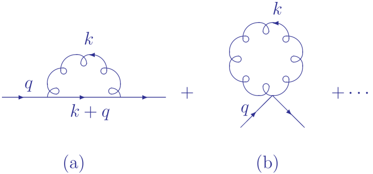
Figure 1: Graviton loop contributions to the scalar propagator. $q$ is the 4-momentum of the scalar.

we have shown in Refs. [9, 10] that the large virtual IR effects in the respective loop integrals for the scalar propagator in quantum general relativity can be resummed to the exact result

$$i\Delta^{\prime}_{F}(k)|_{\text{resummed}}=\frac{ie^{B^{\prime\prime}_{g}(k)}}{(k^{2}-m^{2}-\Sigma^{\prime}_{s}+i\epsilon)}$$ (10)

for   ($\Delta=k^{2}-m^{2}$)

$$\begin{split}B^{\prime\prime}_{g}(k)&=-2i\kappa^{2}k^{4}\frac{\int d^{4}\ell}{16\pi^{4}}\frac{1}{\ell^{2}-\lambda^{2}+i\epsilon}\\ &\qquad\frac{1}{(\ell^{2}+2\ell k+\Delta+i\epsilon)^{2}}\\ &=\frac{\kappa^{2}|k^{2}|}{8\pi^{2}}\ln\left(\frac{m^{2}}{m^{2}+|k^{2}|}\right),\end{split}$$ (11)

where the latter form holds for the UV regime, so that (10) falls faster than any power of $|k^{2}|$. An analogous result [9] holds for m=0. As $\Sigma^{\prime}_{s}$ starts in ${\cal O}(\kappa^{2})$, we may drop it in calculating one-loop effects. It follows that, when the respective analogs of (10) are used for the elementary particles, one-loop corrections are finite. It can be shown actually that the use of our resummed propagators renders all quantum gravity loops UV finite [9, 10]. We have called this representation of the quantum theory of general relativity resummed quantum gravity (RQG).

When we use our resummed propagator results, as extended to all the particles in the SM Lagrangian and to the graviton itself, working now with the complete theory

$${\cal L}(x)=\frac{1}{2\kappa^{2}}\sqrt{-g}\left(R-2\Lambda\right)+\sqrt{-g}L^{\cal G}_{SM}(x)$$ (12)

where $L^{\cal G}_{SM}(x)$ is SM Lagrangian written in diffeomorphism invariant form as explained in Refs. [9, 10], we show in Refs. [9, 10] that the denominator for the propagation of transverse-traceless modes of the graviton becomes

$$q^{2}+\Sigma^{T}(q^{2})+i\epsilon\cong q^{2}-q^{4}\frac{c_{2,eff}}{360\pi M_{Pl}^{2}},$$ (13)

where we have defined

$$\begin{split}c_{2,eff}&=\sum_{\text{SM particles j}}n_{j}I_{2}(\lambda_{c}(j))\\ &\cong 2.56\times 10^{4}\end{split}$$ (14)

with $I_{2}$ defined [9, 10] by

$$I_{2}(\lambda_{c})=\int^{\infty}_{0}dxx^{3}(1+x)^{-4-\lambda_{c}x}$$ (15)

and with $\lambda_{c}(j)=\frac{2m_{j}^{2}}{\pi M_{Pl}^{2}}$ and [9, 10] $n_{j}$ equal to the number of effective degrees of particle $j$. In arriving at (14), we take the SM masses as follows: for the now presumed three massive neutrinos [11], we estimate a mass at $\sim 3$ eV; for the remaining members of the known three generations of Dirac fermions $\{e,\mu,\tau,u,d,s,c,b,t\}$, we use [12, 13] $m_{e}\cong 0.51$ MeV, $m_{\mu}\cong 0.106$ GeV, $m_{\tau}\cong 1.78$ GeV, $m_{u}\cong 5.1$ MeV, $m_{d}\cong 8.9$ MeV, $m_{s}\cong 0.17$ GeV, $m_{c}\cong 1.3$ GeV, $m_{b}\cong 4.5$ GeV and $m_{t}\cong 174$ GeV and for the massive vector bosons $W^{\pm},~{}Z$ we use the masses $M_{W}\cong 80.4$ GeV, $M_{Z}\cong 91.19$ GeV, respectively. We set the Higgs mass at $m_{H}\cong 120$GeV, in view of the limit from LEP2 [14]. We note that (see the Appendix 1 in Ref. [9]) when the rest mass of particle $j$ is zero, such as it is for the photon and the gluon, the value of $m_{j}$ turns-out to be $\sqrt{2}$ times the gravitational infrared cut-off mass [15], which is $m_{g}\cong 3.1\times 10^{-33}$eV. We further note that, from the exact one-loop analysis of Ref.[16], it also follows that the value of $n_{j}$ for the graviton and its attendant ghost is $42$. For $\lambda_{c}\rightarrow 0$, we have found the approximate representation

$$I_{2}(\lambda_{c})\cong\ln\frac{1}{\lambda_{c}}-\ln\ln\frac{1}{\lambda_{c}}-\frac{\ln\ln\frac{1}{\lambda_{c}}}{\ln\frac{1}{\lambda_{c}}-\ln\ln\frac{1}{\lambda_{c}}}-\frac{11}{6}.$$ (16)

These results allow us to identify (we use $G_{N}$ for $G_{N}(0)$)

$$G_{N}(k)=G_{N}/(1+\frac{c_{2,eff}k^{2}}{360\pi M_{Pl}^{2}})$$ (17)

and to compute the UV limit $g_{*}$ as

$$g_{*}=\lim_{k^{2}\rightarrow\infty}k^{2}G_{N}(k^{2})=\frac{360\pi}{c_{2,eff}}\cong 0.0442.$$ (18)

We stress that this result has no threshold/cut-off effects in it. It is a pure property of the known world.

Turning now to the prediction for $\lambda_{*}$, we use the Euler-Lagrange equations to get Einstein’s equation as

$$G_{\mu\nu}+\Lambda g_{\mu\nu}=-\kappa^{2}T_{\mu\nu}$$ (19)

in a standard notation where $G_{\mu\nu}=R_{\mu\nu}-\frac{1}{2}Rg_{\mu\nu}$, $R_{\mu\nu}$ is the contracted Riemann tensor, and $T_{\mu\nu}$ is the energy-momentum tensor. Working then with the representation $g_{\mu\nu}=\eta_{\mu\nu}+2\kappa h_{\mu\nu}$ for the flat Minkowski metric $\eta_{\mu\nu}=\text{diag}(1,-1,-1,-1)$ we see that to isolate $\Lambda$ in Einstein’s equation (19) we may evaluate its VEV(vacuum expectation value of both sides). For any bosonic quantum field $\varphi$ we use the point-splitting definition (here, :  : denotes normal ordering as usual)

$$\begin{split}\varphi(0)\varphi(0)&=\lim_{\epsilon\rightarrow 0}\varphi(\epsilon)\varphi(0)\cr&=\lim_{\epsilon\rightarrow 0}T(\varphi(\epsilon)\varphi(0))\cr&=\lim_{\epsilon\rightarrow 0}\{:(\varphi(\epsilon)\varphi(0)):+<0|T(\varphi(\epsilon)\varphi(0))|0>\}\cr\end{split}$$ (20)

where the limit $\epsilon\equiv(\epsilon,\vec{0})\rightarrow(0,0,0,0)\equiv 0$ is taken from a time-like direction respectively. Thus, a scalar makes the contribution to $\Lambda$ given by

$$\begin{split}\Lambda_{s}&=-8\pi G_{N}\frac{\int d^{4}k}{2(2\pi)^{4}}\frac{(2\vec{k}^{2}+2m^{2})e^{-\lambda_{c}(k^{2}/(2m^{2}))\ln(k^{2}/m^{2}+1)}}{k^{2}+m^{2}}\cr&\cong-8\pi G_{N}[\frac{3}{G_{N}^{2}64\rho^{2}}],\cr\end{split}$$ (21)

where $\rho=\ln\frac{2}{\lambda_{c}}$ and we have used the calculus of Refs. [9, 10]. The standard equal-time (anti-)commutation relations algebra realizations then show that a Dirac fermion contributes $-4$ times $\Lambda_{s}$ to $\Lambda$. The deep UV limit of $\Lambda$ then becomes, allowing $G_{N}(k)$ to run as we calculated,

$$\begin{split}\Lambda(k)&\operatornamewithlimits{\longrightarrow}_{k^{2}\rightarrow\infty}k^{2}\lambda_{*},\cr\lambda_{*}&=-\frac{c_{2,eff}}{960}\sum_{j}(-1)^{F_{j}}n_{j}/\rho_{j}^{2}\cr&\cong 0.232\end{split}$$ (22)

where $F_{j}$ is the fermion number of $j$, $n_{j}$ is the effective number of degrees of freedom of $j$ and $\rho_{j}=\rho(\lambda_{c}(m_{j}))$. We see again that $\lambda_{*}$ is free of threshold/cut-off effects. It is a pure prediction of our world as we know it. In an exactly supersymmetric theory, $\lambda_{*}$ would vanish.

For reference, the UV fixed-point calculated here, $(g_{*},\lambda_{*})\cong(0.0442,0.232)$, can be compared with the estimates in Refs. [3, 4], which give $(g_{*},\lambda_{*})\approx(0.27,0.36)$, with the understanding that the analysis in Refs. [3, 4] did not include the specific SM matter action and that there is definitely cut-off function sensitivity to the results in the latter analyses. What we do see is that the qualitative results that $g_{*}$ and $\lambda_{*}$ are both positive and are significantly less than 1 in size with $\lambda_{*}>g_{*}$ are true of our results as well.

To sum up, we have put Planck scale cosmology [3, 4] on a more rigorous basis. We look forward to possible checks from experiment, to which we return elsewhere [17].

References

- [1] See for example A. H. Guth and D.I. Kaiser, Science 307 (2005) 884, and references therein.
- [2] See for example A. Linde, Lect. Notes. Phys. 738 (2008) 1, and references therein.
- [3] A. Bonanno and M. Reuter, Phys. Rev. D65 (2002) 043508.
- [4] A. Bonanno and M. Reuter, arXiv.org:0803.2546, and references therein.
- [5] O. Lauscher and M. Reuter, hep-th/0205062, and references therein.
- [6] A. Bonanno and M. Reuter, Phys. Rev. D62 (2000) 043008, and references therein.
- [7] D. F. Litim, Phys. Rev. Lett.92(2004) 201301; Phys. Rev. D64 (2001) 105007, and references therein.
- [8] R. Percacci and D. Perini, Phys. Rev. D68 (2003) 044018.
- [9] B.F.L. Ward, hep-ph/0607198.
- [10] B.F.L. Ward, Mod. Phys. Lett. A17 (2002) 237; Mod. Phys. Lett. A19 (2004) 14; J. Cos. Astropart. Phys.0402 (2004) 011; hep-ph/0605054, hep-ph/0503189,0502104, hep-ph/0411050, 0411049, 0410273 and references therein.
- [11] See for example D. Wark, in Proc. ICHEP02, in press; and, M. C. Gonzalez-Garcia, hep-ph/0211054, in Proc. ICHEP02, in press, and references therein.
- [12] K. Hagiwara et al., Phys. Rev. D66 (2002) 010001; see also H. Leutwyler and J. Gasser, Phys. Rept. 87 (1982) 77, and references therein.
- [13] S. Eidelman et al., Phys. Lett.B592 (2004) 1.
- [14] D. Abbaneo et al., hep-ex/0212036; see also, M. Gruenewald, hep-ex/0210003, in Proc. ICHEP02,eds. S. Bentvelsen et al., (North-Holland,Amsterdam, 2003), Nucl. Phys. B Proc. Suppl. 117(2003) 280.
- [15] S. Perlmutter et al., Astrophys. J. 517 (1999) 565; and, references therein.
- [16] G. ’t Hooft and M. Veltman, Ann. Inst. Henri Poincare XX, 69 (1974).
- [17] B.F.L. Ward, to appear.