The star-formation history of $K$-selected galaxies

Abstract

We have studied the $\mu$Jy radio properties of $K$-selected galaxy populations detected in the Ultra-Deep Survey (UDS) portion of the United Kingdom Infrared Telescope (UKIRT) Deep Sky Survey (UKIDSS) using 610- and 1,400-MHz images from the Very Large Array (VLA) and the Giant Metre-wave Telescope (GMRT). These deep radio mosaics, combined with the largest and deepest $K$-band image currently available, allow high-signal-to-noise (S/N) detections of many $K$-selected sub-populations, including sBzK and pBzK star-forming and passive galaxies. We find a strong correlation between the radio and $K$-band fluxes and a linear relationship between star-formation rate (SFR) and $K$-band luminosity. We find no evidence, from either radio spectral indices or a comparison with submm-derived SFRs, that the full sample is strongly contaminated by active galactic nuclei (AGN) at these low flux densities, though this is very difficult to determine from this dataset. The photometric redshift distributions for the BzK galaxies place 37 (29) per cent of pBzK (sBzK) galaxies at $z<1.4$, implying that location on the BzK diagram alone is not sufficient to select samples at $1.4<z<2.5$. The sBzK and pBzK galaxies have similar levels of radio flux density, SFR and specific SFR (SSFR – SFR per unit stellar mass) at $z<1.4$, suggesting there is strong contamination of the pBzK sample by star-forming galaxies. At $z>1.4$, the pBzK galaxies become difficult to detect in the radio stack, though the implied SFRs are still much higher than expected for passively evolving galaxies. It may be that their radio emission comes from low-luminosity AGN. Extremely red objects (EROs) straddle the passive and star-forming regions of the BzK diagram and also straddle the two groups in terms of their radio properties. We find that $K$-bright ERO samples are dominated by passive galaxies and faint ERO samples contain more star-forming galaxies. The star-formation history (SFH) from stacking all $K$-band sources in the UDS agrees well with that derived for other wavebands and other radio surveys, at least out to $z\sim 2$. The radio-derived SFH then appears to fall more steeply than that measured at other wavelengths. The SSFR for $K$-selected sources rises strongly with redshift at all stellar masses, and shows a weak dependence on stellar mass. High- and low-mass galaxies show a similar decline in SSFR since $z\sim 2$.

1 Introduction

There has recently been a large advance in our ability to undertake deep, large-area surveys in the near-infrared (IR) due to the introduction of very large IR-sensitive arrays. Such surveys allow us to collect statistically powerful samples of galaxies selected in the $K$ filter at 2.2 $\mu$m, providing access to the part of the spectral energy distribution (SED) dominated by rest-frame optical light for galaxies at high redshift and by low-mass stars for galaxies at low redshift. Since it is not as strongly affected by dust or biased towards young stars as optical emission, it provides a sample selected approximately on stellar mass ($M_{\rm stellar}$).

There are several classifications for $K$-selected galaxies – extremely red objects (EROs – Elston, Rieke & Rieke 1989), distant red galaxies (DRGs – van Dokkum et al. 2004) and, more recently, BzK galaxies (Daddi et al. 2004). All these selections are colour based and aim to select – via SED shape – particular kinds of galaxies at particular redshifts. The most successful selection appears to be via the BzK technique, where both passive (pBzK) and star-forming (sBzK) galaxies can be selected over the interval $1.4<z<2.5$. In order to investigate the star-formation properties of these galaxies, we will exploit deep radio imaging and stack the IR positions into the radio data to derive averaged radio properties at $\mu$Jy levels for various classes of $K$-selected sources.

The strong correlation between far-IR (FIR) and radio emission (Helou et al. 1985) in local star-forming galaxies (SFGs) has allowed the use of radio surveys as a means to quantify star-formation activity in a manner immune to the obscuring effects of dust. The FIR emission is believed to be produced by dust which has been heated by the ultraviolet (UV) photons from massive stars. These stars end their lives as supernovae and the remnants of these explosions produce the synchrotron radio emission. Thus both the FIR and radio trace the rate of formation of massive stars. Radio emission is unaffected by dust, unlike optical and UV photons, and so the radio provides a powerful tool for studying star formation at high angular resolution in a relatively unbiased way.

The radio source counts above 1 mJy are dominated by AGN, the powerful Fanaroff-Riley-ii (FR ii – Fanaroff & Riley 1974) sources giving way to the less powerful (but still radio-loud) FR i AGN as the flux-density threshold approaches $S_{\rm 1,400}\sim 1$ mJy (Windhorst et al. 1985; Willott et al. 2002). The evolution of these two types of radio-emitting AGN differs, with FR ii sources undergoing strong evolution (Dunlop & Peacock 1990; Willott et al. 2001) while FR i sources undergo a weaker evolution or possibly maintain a constant co-moving space density (Clewley & Jarvis 2004; Sadler et al. 2007; Rigby, Best & Snellen 2008). The contribution of these sources to the radio source counts should continue to be a power law to fainter flux densities (Jarvis & Rawlings 2004). At flux densities below 1 mJy, the radio counts are observed to flatten and a new population of sub-mJy radio sources, originally thought to be SFGs, becomes apparent (Condon 1984). There is the possibility, however, that the sub-mJy population could also consist of ‘radio-quiet’ AGN (Jarvis & Rawlings 2004) – i.e. AGN with a low ratio of radio to optical/X-ray luminosity which still contain a super-massive black hole accreting at a high rate, contributing to the radio emission.

The exact mix of AGN versus star formation at sub-mJy levels is still the subject of lively debate (see Ibar et al. 2008 and references therein). The first deep radio surveys ascribed the bulk of the sub-mJy activity to SFGs (Hopkins et al. 1998; Gruppioni et al. 1999; Richards 2000) though further investigations with more complete optical, X-ray and high-resolution radio imaging have shown a very mixed picture. A deep, narrow 5-GHz survey in the Lockman Hole (Ciliegi et al. 2003) found a flattening of radio spectral indices at faint flux limits, consistent with an increasing fraction of AGN. They also found that a substantial fraction (50 per cent) of $S_{\rm 5GHz}>50$-$\mu$Jy sources are early-type galaxies. Using radio morphologies to distinguish radio AGN from SFGs suggests a mix of both types at faint flux levels across a broad range of redshift and radio luminosity (Richards et al. 2007), although approaching this with sufficient resolution awaits the commissioning of e-MERLIN. Simpson et al. (2006) studied the the nature of the sub-mJy population ($S_{\rm 1,400}>100\,\mu$Jy) in the Subaru-XMM-Newton Deep Field (SXDF) and concluded that radio-quiet AGN make a significant contribution to the counts at $100<S_{\rm 1,400}<300\,\mu$Jy. This conclusion is supported by Smolčić et al. (2008) in the COSMOS field, where they find that 50–60 per cent of $z<1.3$ galaxies with $50<S_{\rm 1,400}<70\,\mu$Jy are AGN. In contrast, a recent study by Seymour et al. (2008), using VLA and MERLIN images, has been able to separate radio sources into AGN and SFGs on the basis of radio morphology, spectral index and radio/near-IR and mid-IR/radio flux density ratios. They find that SFGs dominate the counts at $\sim$50$\mu$Jy and account for the majority of the upturn in the radio counts below 1 mJy. An extrapolation of their figure 3 to the flux densities we are typically probing here ($\sim 10\,\mu$Jy) would suggest that AGN are far outnumbered by SFGs and should not be a major concern in this stacking.

As we are probing the radio population at flux density levels an order of magnitude fainter than existing studies, it is impossible to know – a priori – the relative contributions to the radio flux of accretion and star formation for a given population. This difficulty in distinguishing between star-formation- and AGN-induced radio emission will potentially present us with biases in our results. For instance, if we assume all of the radio emission is due to star formation, then we will over-estimate the true SFRs. If, in the hope of excising AGN, we discount all sources with certain values of $L_{\rm 1,400}$ or ratios of radio/optical flux, then we will bias ourselves as extreme starbursts will also have high $L_{\rm 1,400}$ (Ivison et al. 2002) and high radio/optical ratios. Given the findings of Richards et al. (2007), that radio-emitting AGN appear at all radio luminosities and radio/optical ratios, we do not feel that such cuts to the sample can be justified. We will simply include all sources, placing an upper limit on the star-formation activity, investigating along the way whether there are any other indications as to the nature of the radio emission.

The layout of the paper is as follows: §2 describes the radio and IR observations. §3 describes the stacking procedure used in the radio. In §4 we present the results of the stacks while in §5 we investigate the possible contamination from AGN using radio spectral indices and submm stacks. In §6 we present the radio-derived SFH of $K$-selected galaxies out to $z=4$ and also investigate their specific SFRs as a function of mass and redshift.

The cosmology used throughout is $\Omega_{\Lambda}=0.73$, $\Omega_{m}=0.27$ and $H_{0}=71$ km s^-1 Mpc^-1.

2 Observations

2.1 IR data and photometric redshifts

The catalogue used in this paper was selected from the ongoing UDS, which is the deepest of the five surveys that comprise UKIDSS (Lawrence et al. 2007), exploiting the IR Wide-Field Camera (WFCAM – Casali et al. 2007) on UKIRT. The UDS will cover 0.8 deg² in $J,H,K$ to eventual 5$\sigma$ limits of 26.9, 25.9, 24.9 mag (we use AB magnitudes throughout, unless stated otherwise), built from a 4-point mosaic of WFCAM. Stacking, mosaicing and quality control for the UDS was performed using a different recipe to the standard UKIDSS pipeline, and is described fully in Almaini et al. (in preparation). In this work we used data from the DR1 release (Warren et al. 2007), which includes $J$ and $K$ images reaching 5-$\sigma$ depths of $K=23.6$ and $J=23.7$ (2-arcsec diameter apertures). These images have median seeing of 0.85 and 0.75 arcsec (fwhm) in $J$ and $K$, respectively, with astrometry (calibrated against 2MASS stars) accurate to $\sigma<0.05$ arcsec. Photometry is also uniformly accurate to $<$2 per cent r.m.s. in both bands. We performed source extraction using the Sextractor software (Bertin & Arnouts 1996), using simulations to optimise source completeness, further details of which are described in Foucaud et al. (2007). Objects which were saturated, in noisy regions or defined as compact ($K<19.9$ and with a 50 per cent light radius around the point spread function – PSF) were not included in the catalogue. The detection completeness at $K=23.0$ in 2-arcsec diameter apertures is estimated to be $\sim$80 percent. At $K<22.5$ completeness is $\sim$100 percent.

We matched the UDS $K$-selected catalogue to deep optical data in this field from the Subaru XMM-Newton Deep Field survey (Furasawa et al. 2008) in five broad-band filters to 3-$\sigma$ depths of $B=28.4,V=27.8,R=27.7,i^{\prime}=27.7,z^{\prime}=26.6$ (again, 2-arcsec diameter apertures).

This deep multi-wavelength coverage of the UDS allowed us to model the galaxy SEDs in detail, as described in Cirasuolo et al. (2008). The SED fitting procedure, to derive photometric redshifts, was performed with a code based largely on the public package Hyperz (Bolzonella, Miralles & Pelló 2000) and exploits reliable photometry in 16 broad bands from far-UV to the mid-IR. Both empirical (Coleman, Wu & Weeman 1980; Kinney et al. 1996; Mignoli et al. 2005) and synthetic templates (Bruzual & Charlot 2003) were used to model the galaxy SEDs, including a prescription for dust attenuation (Calzetti et al. 2000) and Lyman-series absorption due to the H i clouds in the intergalactic medium, according to Madau (1995).

For the $\simeq$1,200 galaxies in the UDS with reliable spectroscopic redshifts, the agreement of the photometric redshifts is good over the full redshift range, $0<z<6$. The distribution of the $|\Delta z|/(1+z)\equiv|(z_{\rm spect}-z_{\rm phot})|/(1+z_{\rm spect})$ has a mean consistent with zero (0.008), a standard deviation, $\sigma=0.034$, and clear outliers make up less than 2 per cent of the total. A comparison of $z_{\rm spec}$ versus $z_{\rm phot}$ can be found in fig. 2 of Cirasuolo et al. (2008). This accuracy is comparable to the best available from other surveys such as GOODS and COSMOS (Caputi et al. 2006a; Grazian et al. 2006; Mobasher et al. 2007).

2.2 Radio observations

The radio data used here are described by Ivison et al. (2007a) and Ibar et al. (2008). Briefly, we employed the National Radio Astronomy Observatory’s (NRAO) VLA at 1,400 MHz, with an effective bandwidth of 4$\times$7$\times$3.125 MHz (via correlator mode ‘4’) and central frequencies in the two IF pairs of 1,365 and 1,435 MHz. This provided a good compromise between high sensitivity (via greater bandwidth) and the effect of bandwidth smearing (BWS), which scales with channel width and distance from the pointing centre. We obtained data at three positions, the vertices of an equalatoral triangle with 15-arcmin sides, with a 9:3:1 combination of data from the VLA’s A:B:C configurations. This yielded a synthesised beamwidth of around 1.7 arcsec fwhm. The noise level varies across the mosaic: 165 arcmin² at $<$7 $\mu$Jy beam^-1 in Stokes I, 750 arcmin² at $<$10 $\mu$Jy beam^-1 and 1345 arcmin² at $<$15 $\mu$Jy beam^-1. A total of 563 sources were detected at $>$5 $\sigma$.

When imaging, we used only those data within a radius of each pointing centre where the dimensionless BWS term, $\beta$ (fractional bandwidth $\times$ radius, the latter in units of fwhm), was $<$1.225. This ensured the reduction in peak flux density due to BWS — a pernicious effect which can lead to the complete loss of real sources from radio catalogues — was always $<$37 per cent ($(1+\beta^{2})^{-0.5}$). We then calculated error-weighted values of $\beta$ at every point in the final 3-position mosaic, using these to correct the flux densities extracted at the position of each galaxy.

3 Stacking the radio flux of $K$-selected populations

3.1 IR-selection criteria

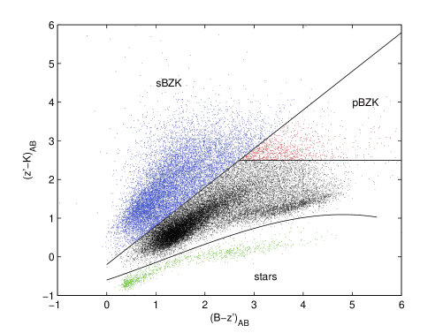
Figure 1: BzK colour-colour diagram showing the location of the different samples. The stellar branch was removed before stacking.

The selection criteria for the galaxies to be stacked were $K\leq 23.0$ and total $\chi^{2}<10$ for the photometric redshift. This prevents the results becoming contaminated with unreliable sources or redshifts. Sources had to lie in the overlap region between the UDS $K$ data, the SuprimeCam optical images and the VLA 1,400-MHz image (1311.1 arcmin²). The total number of $K$-selected sources in this region, meeting the above criteria is 23,185 of which 440 have radio counterparts at $>$5 $\sigma$.

A BzK diagram of the sample meeting the $K$ and photometric redshift selection criteria is shown in Fig. 1. This splits into several sub-samples based on the BzK colour cut (Daddi et al. 2004), where BzK $\equiv(z^{\prime}-K)-(B-z^{\prime})$:

1. All galaxies: all objects classified as galaxies (and not lying on the stellar branch of the BzK diagram) meeting the selection criteria. All points on Fig. 1, except the green stars.

2. Star-forming, high-redshift: using the sBzK selection of $BzK\geq-0.2$ we select a sample of 6,626 high-redshift SFGs. These are the blue points on Fig. 1.

3. Passive, high-redshift: using the pBzK selections of $BzK<-0.2$ and $(z^{\prime}-K)>2.5$ we select a sample of 542 high-redshift passive galaxies. These are the red points on Fig. 1.

4. Non-BzK galaxies: all of the black points in Fig. 1. Generally galaxies at lower redshifts than the BzK sources.

5. EROs: defined as all objects with $(R-K)_{\rm AB}>3.6$. Generally these span the space overlapping pBzK, sBzK and non-BzK at the top right of the BzK diagram (see Fig. 7).

Note that a sparse stellar branch is visible on the plot because the BzK diagram is efficient at selecting stars up to 1 mag deeper than the compactness selection used to make the $K$ catalogue.

These colour selections are untested at the depths of the UDS and we will investigate their reliability as best we can using the radio data and photometric redshifts. We also note that the sBzK star-forming sample is known to contain a fraction of AGN (Daddi et al. 2004; Reddy et al. 2005) and we will discuss this in more detail in §5.

3.2 Radio Stacking

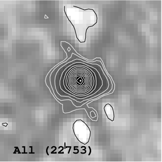
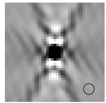
Figure 2: Left: $16\times 16$-arcsec² postage-stamp image of all $K$-selected galaxies meeting the selection criteria. The number of galaxies in the stack is indicated on the image. Contours are at $-3,3,4,6,10,15$ and then in steps of $+5\sigma$. S/N is so high that the lobes of the dirty beam can be seen. Right: A dirty beam, averaged over the three VLA pointings, is shown alongside at the same scale for comparison. The size of the VLA restoring beam ($\rm FWHM=1.7$-arcsec) is shown in the bottom right corner.

To perform the stacking we measured the noise-weighted mean and median of the pixels on the radio image corresponding to the positions of the $K$-band sources. As the radio image has units of Jy beam^-1, this pixel stacking gives the total flux of a source which is no larger than the beam. We only considered regions on the radio image with $\sigma_{\rm 1,400}\leq 20\,\mu$Jy. For the mean stacks we excluded pixels with $\rm|S/N|\geq 5$ but for the median we included all sources. The errors on the median were calculated using the distribution of flux densities, following Gott et al. (2001). While there is often a small difference between the mean and median value, these are usually within the $\sigma_{\rm 1,400}$ uncertainties in each case. The median (Gott et al. 2001) is a more robust measure of a population which may deviate from a normal distribution (as a population containing detections will do) and so, in general, we prefer the median. This is important in the samples which we later bin by stellar mass or absolute $K$ mag, since as many as 30 per cent of the sources may be detected at $>$5 $\sigma$ in the highest bins of stellar mass. To discount these detections (as done when computing the mean) would not produce a representative average for this high-mass sub-sample; with the median we can use the same statistic whatever the fraction of detections.

We corrected the final mean or median values for the effect of bandwidth smearing (as described in §2.2) by multiplying the value by the mean or median BWS term. The mean and median BWS term was calculated in the same way as the mean and median flux density. The reason the correction was applied to the final stacked value rather than the individual pixel values is explained next. The BWS correction should not affect the noise on the map; it merely corrects for the reduction in peak flux density due to BWS. However, in stacking (where we expect no detections) our stacked values can be positive or negative, thus the effect of a BWS correction applied to each pixel would be to increase the effective $\sigma_{\rm 1,400}$ on the resulting pixel flux distribution. If we multiply each pixel by the BWS value, but not the noise on that pixel, then we are artificially increasing the S/N of every pixel. This has two consequences: first, we finish with statistics which are not Gaussian (e.g. more $>$3-$\sigma$ peaks on the stacked maps than expected); second, as we are rejecting $\rm|S/N|\geq 5$ points from the stack, we have fewer points to stack. If we decide to increase the noise at every point by the BWS factor to counter these problems then, again, we have less sources to stack as a larger fraction of the map then appears to have $\sigma_{\rm 1,400}>20\,\mu$Jy. Our solution was to multiply both the final flux density in the stack and the final error by the averaged BWS. This leaves us with the correct number of sources and Gaussian statistics (so the reliability of the detections is intuitive to calculate).

Table 1: Integrated fluxes and fitted sizes of postage stamps.

Redshift	$K$ cut	$\bar{S}_{\rm 1,400}$	$S_{\rm 1,400}^{\rm med}$	$S_{\rm 1,400}^{\rm int}$	Ratio	Size
		($\mu$Jy)	($\mu$Jy)	($\mu$Jy)		(arcsec)
$z<0.2$	$K\leq 23.0$	$3.34\pm 0.42$	$2.99\pm 0.74$	$7.64\pm 1.59$	$2.29\pm 0.56$	$3.96\,(0.66)\times 2.66\,(0.44)$
$z<0.7$	$K\leq 23.0$	$4.82\pm 0.15$	$4.67\pm 0.23$	$7.04\pm 0.43$	$1.46\pm 0.10$	$2.52\,(0.11)\times 2.34\,(0.10)$
$z>0.7$	$K\leq 23.0$	$6.44\pm 0.11$	$6.15\pm 0.19$	$8.24\pm 0.35$	$1.28\pm 0.06$	$2.32\,(0.07)\times 2.17\,(0.06)$
$z>0.2$	$K\leq 21.5$	$10.13\pm 0.16$	$10.44\pm 0.28$	$14.15\pm 0.56$	$1.40\pm 0.06$	$2.43\,(0.07)\times 2.28\,(0.06)$
$z>0.2$	$21.5<K\leq 23.0$	$4.15\pm 0.11$	$3.90\pm 0.17$	$5.07\pm 0.27$	$1.22\pm 0.07$	$2.29\,(0.08)\times 2.09\,(0.07)$

We performed exactly the same analysis at random positions to check that there were no systematic effects in the radio map which might lead us to a positive flux. Flux was stacked at 21,000 random positions and this stack was repeated 1,000 times. The mean of the 1,000 mean values was 0.015 $\mu$Jy with $\sigma_{\rm 1,400}=0.13\,\mu$Jy and the mean of the 1,000 medians was $-0.009\,\mu$Jy with $\sigma_{\rm 1,400}=0.17\,\mu$Jy. This is consistent with zero and well below any fluxes quoted from a stack of $K$-selected objects.

We also took a $41\times 41$-pixel region around every IR position and stacked this to produce a noise-weighted mean image stack (see Fig. 2). We excluded any pixels on the radio image with a high noise level ($>$20 $\mu$Jy) or with a value of $\rm|S/N|\geq 5$). These postage-stamp images are not corrected for BWS as the integrated flux is not affected by band-width smearing. The integrated flux is measured directly from the postage stamp images using jmfit in $\cal AIPS\/$and also includes any systematic effects due to positional uncertainty in the $K$-band positions, as well as any flux from sources which are larger than the beam. We made stacks of samples cut in redshift and $K$ to see if either produced a more significant difference to the pixel stacks, as we might expect positional uncertainty to be greater at fainter $K$ and source sizes to be larger at lower redshift. The results are listed in Table 1. We found that samples which were cut at $z>0.2$ gave consistent ratios between the $\cal AIPS\/$ integrated fit and the mean from the pixel stack. Thus positional errors on the $K$-selected sources did not vary significantly as a function of $K$ mag to our limit of $K=23.0$. The largest effect seems to be from partially resolved sources at low redshifts. The average ratio of integrated to BWS-corrected mean-weighted-stacked flux density is 1.31 for $z>0.2$ and 2.29 for $z<0.2$. A further correction needs to be made to this integrated flux for the fact that these radio stacks are not ‘cleaned’. In the VLA image, only sources visible to the eye were cleaned, via clean boxes placed by hand. Sources at the low flux density levels found here resemble the dirty beam with flux (both positive and negative) in their sidelobes (see Fig. 2). We looked at the differences between a source fitted in a cleaned map compared to a dirty map and found the average factor between the clean-fitted flux to dirty-fitted flux to be 1.14. Thus the total correction we need to make to our fluxes is $1.14\times 1.31=1.49$ for $z>0.2$ and $1.14\times 2.29=2.61$ for $z<0.2$. Fluxes labelled $S_{\rm 1,400}^{\rm int}$ have been corrected in this way. All derived quantities in figures and tables ($L_{\rm 1,400}$, SFR, SSFR) have been corrected.

We also checked that the noise integrated down as expected following Poissonian statistics by measuring the noise in the stacked postage-stamp images around the detected sources and on the Monte-Carlo images. This confirmed that the noise does integrate down as expected, i.e. as $\sigma/\sqrt{N_{\rm sources}}$.

3.3 Deriving SFRs and luminosities

We can use photometric redshifts at the time of stacking the radio data to derive rest-frame 1,400-MHz luminosities, $L_{\rm 1,400}$, and SFRs for the galaxies. The 1,400-MHz luminosity is calculated for each pixel based on the flux at that pixel and the redshift of the galaxy being stacked, using

$$L_{\rm 1,400}\,({\rm W\,Hz^{-1}})=9.52\times 10^{18}\,S_{\rm 1,400}\,D_{\rm L}^{2}\,4\pi(1+z)^{-0.2}$$

where $D_{\rm L}$ is the luminosity distance of an individual galaxy in Mpc and $S_{\rm 1,400}$ is the 1,400-MHz flux density of the pixel corresponding to that galaxy in Jy. This assumes a radio spectral index ($S_{\nu}\propto\nu^{\alpha}$) of $\alpha=-0.8$.

The median 1,400-MHz luminosity is then the median of the luminosities for the individual pixels. We note that this is not the same as taking the median stacked flux and median redshift and applying the above equation, since the median redshift of the sub-sample may not be that at which the peak of the radio emission is being produced.

The SFR is then calculated from the median 1,400-MHz luminosity in two ways. First, following Condon (1992), Haarsma et al. (2000) and Condon et al. (2002), we have

$$\dot{\rho_{\ast}}({\rm M_{\odot}\,yr^{-1}})=\left[\frac{5.5\times L_{\rm 1,400}}{(5.3\times 10^{21}\times\nu^{-0.8})+(5.5\times 10^{20}\times\nu^{-0.1})}\right]$$

where $\nu$ is the frequency in GHz. For 1,400 MHz, this becomes

$$\dot{\rho_{\ast}}({\rm M_{\odot}\,yr^{-1}})=1.2006\times 10^{-21}L_{\rm 1,400}$$

Second, following Bell (2003), we have

$$\dot{\rho_{\ast}}({\rm M_{\odot}\,yr^{-1}}) = 5.52\times 10^{-22}\,L_{\rm 1,400},\,\,\,\,\,L>L_{c}$$

$$= \frac{5.52\times 10^{-22}\,L_{\rm 1,400}}{0.1+0.9(L/L_{c})^{0.3}},\,\,\,\,L\leq L_{c}$$

where $L_{c}=6.4\times 10^{21}\,\rm{W\,Hz^{-1}}$.

Both conversions assume a Salpeter-like initial mass function (IMF) with $\Psi(M)\propto M^{-2.35}$ and a mass range of $0.1-100\,\rm{M_{\odot}}$. The study by Bell (2003) suggests that the radio does not trace star formation as effectively at low values of $L_{\rm 1,400}$ because the non-thermal radio emission is suppressed by a factor of 2–3 in $\sim L_{\ast}/100$ galaxies relative to $L_{\ast}$. The Bell (2003) conversion thus boosts the radio SFR at low $L_{\rm 1,400}$ values by a factor $\sim 2$ compared to Condon (1992); however, the overall normalisation of SFR is lower than that used by Condon (1992).

4 Results

Table 2: Stacked radio properties at 1,400-MHz for $K$-selected samples.

Sample	N	% det	$\bar{S}_{\rm 1,400}$	$S_{\rm 1,400}^{\rm med}$	$S_{\rm 1,400}^{\rm int}$	$L_{\rm 1,400}$	SFR	SSFR	$\langle z\rangle$
			($\mu$Jy)	($\mu$Jy)	($\mu$Jy)	($\rm{W\,Hz^{-1}}$)	($\rm{M_{\odot}\,yr^{-1}}$)	($\rm{Gyr^{-1}}$)
All galaxies	23,185	1.9	$5.90\pm 0.09$	$5.66\pm 0.15$	$8.43\pm 0.22$	$1.34\times 10^{22}$	$16.0\pm 0.6$	$1.137\pm 0.042$	0.96
Non-BzK	16,048	1.7	$5.30\pm 0.11$	$4.95\pm 0.17$	$7.38\pm 0.25$	$1.06\times 10^{22}$	$8.5\pm 0.4$	$0.694\pm 0.031$	0.72
sBzK	6,626	2.1	$7.42\pm 0.17$	$7.47\pm 0.25$	$11.13\pm 0.37$	$1.28\times 10^{23}$	$153.6\pm 6.7$	$5.05\pm 0.22$	1.55
pBzK	542	3.9	$5.97\pm 0.57$	$6.72\pm 1.02$	$10.01\pm 1.52$	$1.11\times 10^{23}$	$131.0\pm 18.6$	$2.38\pm 0.39$	1.49
EROs	2,905	4.0	$7.86\pm 0.25$	$7.94\pm 0.49$	$11.83\pm 0.73$	$1.01\times 10^{23}$	$121.1\pm 6.7$	$2.49\pm 0.13$	1.42
Stellar	617	0	$0.13\pm 0.56$	$0.39\pm 0.78$	..	..	..	..	..

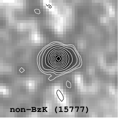
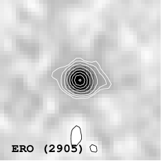
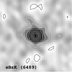
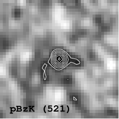
Figure 3: Postage-stamp images of the 1,400-MHz radio stacks for non-BzK, ERO, sBzK and pBzK galaxies in the UDS. Numbers in parenthesis denote the number of sources in each stack. Contours for non-BzK, ERO and sBzK galaxies are plotted at $-3,3,4,6,10,15$ and then in steps of $+5\sigma$, while for pBzK galaxies they are plotted at $-3,3,4,5$ and then in steps of $+1\sigma$. Pixels deviating by more than $\pm 5\sigma$ from the mean have been removed.

Figure 4: Photometric redshift distributions for the $K$-selected samples discussed in the paper.

Table 2 shows the results for each sample and for each stacking method. All four sub-sets of $K$-selected galaxies (ERO, non-BzK, sBzK and pBzK) are significantly detected in the stacks, their postage-stamp stacked images are shown in Fig. 3.

The BzK selection (Daddi et al. 2004) is designed to select either star-forming (sBzK) or passively-evolving (pBzK) galaxies in the redshift range $1.4<z<2.5$. We have taken the colour cut used by Lane et al. (2007), as shown in Fig. 1, which gives us samples of 6,626 sBzK and 542 pBzK galaxies that match the selection criteria and overlap with our radio data. This is by far the largest sample of such galaxies to be stacked in the radio to date.

The redshift distributions for the various samples are shown in Fig. 4. It is immediately apparent that the distributions for BzK galaxies have tails at redshifts higher and lower than the range in which they are designed to lie. At $z<1.4$, this amounts to a fraction of 37 (29) per cent for pBzK (sBzK) galaxies. There are, of course, uncertainties in the photometry which may shift objects in and out of the BzK regions and, for pBzK, the distribution of colours means that more galaxies are likely to scatter in rather than out, accounting for the raised fraction compared to sBzK galaxies. There may also be errors in the photometric redshifts which place some galaxies at a spuriously low redshift. For sBzK galaxies, the $z<1.4$ objects mostly lie along the boundary with non-BzK objects, suggesting that photometric scatter is the main cause of the low-redshift tail. For pBzK galaxies, however, the $z<1.4$ objects fill the same region of colour space as those at $z>1.4$. We will investigate the radio properties of BzK galaxies at all redshifts to see if there are any differences in the $z<1.4$ populations which are contaminating the BzK space. We note that a spectroscopic study by Popesso et al. (2008) also finds that 23 percent of sBzK lie at $z<1.4$. The number of pBzK in their sample is too small to produce a reliable measure of the fraction at low redshift.

In Fig. 5 (left) we show the median flux of BzK galaxies as a function of redshift. The average 1,400-MHz flux density of sBzK galaxies is roughly constant (or slowly rising) over the interval $0.6<z<3.0$, implying a strong evolution in luminosity. For pBzK galaxies there is a dramatic change in the average radio emission from $0.7<z<1.4$ to $1.4<z<2.5$. At $z<1.4$, the pBzK galaxies are relatively bright radio emitters, and are in fact more luminous at this redshift than sBzK galaxies. At $z>1.4$, their radio emission falls to approximately half that of sBzK galaxies. This is the first piece of evidence that the pBzK sample (as defined by the BzK diagram) is not a homogeneous population of passive galaxies. The low-redshift tail cannot be due to photometric errors as the radio properties should then be consistent across the redshift boundary, which they clearly are not. In Fig. 5 (right) we also plot median $L_{\rm 1,400}$ against redshift for the sBzK and pBzK samples. The flat flux-density-redshift trend for sBzK galaxies in Fig. 5 (left) translates into a steep rise of $L_{\rm 1,400}$ with redshift. In contrast, the pBzK sample behaves quite differently, with median $L_{\rm 1,400}$ falling slightly over the range $0.7<z<2.5$ before rising dramatically at higher redshifts (in line with sBzK galaxies). The radio luminosity of pBzK galaxies is higher than that of sBzK galaxies at $0.7<z<1.4$; however, the pBzK galaxies are also more luminous in $K$ over this redshift interval. The elevated luminosity of the pBzK galaxies in this redshift bin is due to the correlation between radio and $K$ fluxes and luminosities (see Fig. 6 and  10). Indeed, the ratio of radio to $K$ fluxes in sBzK and pBzK galaxies at $0.7<z<1.4$ is the same (see Fig. 6). pBzK galaxies are also more luminous in $K$ than sBzK galaxies in the $1.4<z<2.5$ bin. This means that the difference between the sBzK and pBzK galaxies in this bin in Fig. 5 (right) is intrinsically larger when normalised to $K$ luminosity than is shown here.

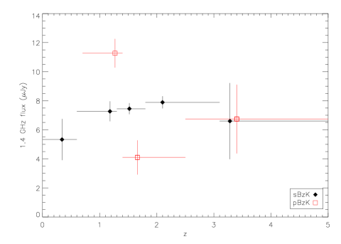
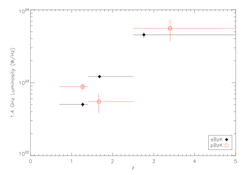
Figure 5: Left: Stacked median flux of BzK galaxies as a function of redshift. Solid black diamonds are sBzK galaxies and red open squares are pBzK galaxies. The sBzK galaxies show a roughly constant flux with increasing redshift while the pBzK galaxies suffer a dramatic reduction in radio flux in the $1.4<z<2.5$ range. This plot argues that the $z<1.4$ pBzK galaxies are not merely redshift outliers but are a physically distinct population. Right: Stacked median luminosity of BzK galaxies as a function of redshift, same symbols as before. The luminosity of pBzK galaxies drops over the interval $0.7<z<2.5$ whereas for sBzK it is rising strongly.

.

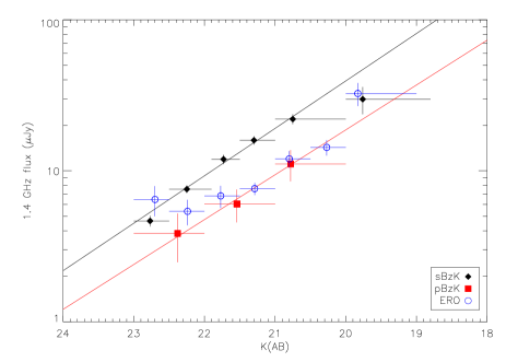
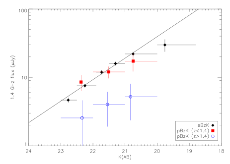
Figure 6: Relationship between $K$ and median stacked 1,400-MHz flux density for all galaxies (top) and BzK and ERO galaxies (middle). Best linear fits are plotted. There is no power-law fit for EROs. Both sBzK and pBzK galaxies have a similar slope with $S_{\rm 1,400}\propto S_{K}^{0.74-0.79}$, though the pBzK sample shows less radio flux density at a given $K$ mag. EROs seem to follow a similar trend to pBzK galaxies at $K>21.5$, while at fainter fluxes the correlation with $K$ seemingly breaks down. In the full sample and the ERO sample, the median redshift increases as $K$ mag increases. Bottom: pBzK galaxies are split into two redshift bins, $z<1.4$ and $1.4<z<2.5$ matching the transition seen in Fig. 5. The low-redshift pBzK galaxies are seen to follow the same radio-$K$ relation as the sBzK galaxies, supporting the idea that they are star-forming interlopers. The pBzK galaxies at $1.4<z<2.5$ are not detected significantly in the radio and have a radio-$K$ relation offset from that of sBzK and low-redshift pBzK galaxies.

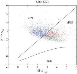
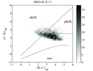
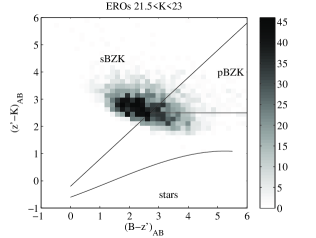
Figure 7: Location of EROs on the BzK diagram. The position of the EROs (left) generally straddles the sBzK and pBzK galaxies as well as the non-BzK region. Brighter EROs (middle) are more likely to lie in the ‘passive’ part of the diagram, fainter EROS (right) are more likely to be sBzK galaxies.

In Fig. 6 we show the correlation between $K$ mag and $S_{\rm 1,400}^{\rm med}$ for the full sample (top) and the BzK and ERO galaxies (middle). There is a strong trend, with $S_{\rm 1,400}\propto S_{K}^{0.53}$ for the full sample, and a steeper relationship for the sBzK galaxies of $S_{\rm 1,400}\propto S_{K}^{0.79}$ and for the pBzK galaxies of $S_{\rm 1,400}\propto S_{K}^{0.74}$. The difference in slope is possibly due to the fact that, for the full sample, the galaxies in the fainter $K$ bins have higher median redshifts than the brighter bins. On the other hand, the BzK galaxies are selected by colour to lie in a particular redshift range and so the median redshifts are approximately the same for all $K$ bins. If the changes in redshift are responsible for the different slopes then the flatter slope indicates that the radio flux density is falling less quickly with redshift compared to the $K$ flux. Fig. 6 shows that the passive early-type pBzK galaxies have a lower radio/$K$-band flux ratio than the star-forming sBzK galaxies. The fact that the slopes are similar for the pBzK and sBzK samples suggests that the mechanism responsible for the radio emission is similar for each class of galaxy (or at least depends on $K$ in the same way). This is as one would expect if pBzK samples contain a fraction of contaminating SFGs which dominate their radio signal. We can follow this idea further by plotting $S_{\rm 1,400}$ versus $K$ mag for subsets of pBzK galaxies, split by redshift. pBzK galaxies at $z<1.4$ have larger 1,400-MHz fluxes and luminosities than those at $1.4<z<2.5$, as shown in the bottom panel of Fig. 6 where the black points are the sBzK sample, the red points are the pBzK galaxies at $z<1.4$ and the blue points are pBzK galaxies at $1.4<z<2.5$. It is now clear that the $z<1.4$ pBzK follow the same $S_{\rm 1,400}$ versus $K$ mag relation as the sBzK galaxies, supporting our hypothesis that they are star-forming interlopers in pBzK colour space. The remaining ‘bona fide’ pBzK galaxies at $1.4<z<2.5$ are shown to have much less radio emission at a given $K$ mag than either sBzK or $z<1.4$ pBzK galaxies. There is not enough signal to determine a slope to the high-redshift pBzK data. The remaining radio flux from the high-redshift pBzK galaxies could come either from a much lower-level contamination by SFGs, or from AGN. We will investigate these two possibilities in §5.

The EROs are a heterogeneous sample. At brighter $K$ mags ($K>21.5$) they match the trends of the pBzK galaxies, but at fainter $K$ mags the correlation between radio and $K$ seems to break down (Fig. 6-middle). In the BzK diagram (Fig. 7), the EROs typically straddle the sBzK and pBzK colour range. Bright EROs have redder $(B-z^{\prime})$ colours and so overlap more with the passive region on the BzK plot. Fainter EROs are more aligned with the sBzK part of the diagram. The point at which the EROs depart from the pBzK relationship is similar to the magnitude of the break in the ERO number counts at $K=20.9-21.9$ (McCarthy et al. 2001; Smith et al. 2002). This is further strong evidence that EROs are not a homogeneous population, and the passive/star-forming split in an ERO sample will depend strongly on the $K$-band selection limit for the sample. This has been noted previously by Smail et al. (2002).

Various colour-selected samples have previously been stacked at 1,400 MHz: BzK (Daddi et al. 2005) and EROs (Georgakakis et al. 2006; Simpson et al. 2007; Ivison et al. 2007b). When we account for the differing $K$ limits of the various samples using Fig. 6 we find good agreement between our ERO and BzK values and those in the literature. We will not discuss EROs further as the BzK colour selection provides a cleaner separation of high-redshift star-forming and passive galaxies.

5 Reliability of radio emission as a tracer of star formation

Integral to this paper is the assumption that we can use the 1,400-MHz radio emission as a tracer of star formation. The main reason why this may not be a valid assumption is the presence of radio-emitting AGN in the sample at flux densities below the detection limit. Even after removing the $z<1.4$ contaminants – almost certainly SFGs – we have already seen that galaxies selected to be passive from the BzK diagram have a residual level of radio emission which could be due to either persistent, low-level contamination by SFGs or due to radio-emitting AGN in pBzK galaxies. The sBzK galaxy population is known to consist of star-forming galaxies and some AGN. Smolčić et al. (2008) show that Seyfert 2 galaxies at $z>1.4$ can lie in the sBzK region of the diagram, while Daddi et al. (2004) and Reddy et al. (2005) have both detected X-ray-bright AGN in the sBzK region. The contamination rate from X-ray-emitting AGN was determined by Reddy et al. (2005) to be 31 per cent for $19.9\leq K\leq 21.9$, 9 per cent for $21.9\leq K\leq 22.4$ and 3 per cent for $22.4\leq K\leq 22.9$. Reddy et al. also compared SFRs derived from X-ray stacking with and without the detected X-ray sources and found their SFR estimates decreased by 13 per cent at $19.9\leq K\leq 21.9$, 3 per cent for $21.9\leq K\leq 22.4$ and 4 per cent for $22.4\leq K\leq 22.9$. After excluding X-ray-detected sources, their X-ray stack showed no hard-band detection. They took this to indicate insignificant contamination from low-luminosity AGN. Given that most of our sources (75 per cent) are fainter in $K$ than the bins where Reddy et al. find significant AGN contamination, we do not expect a problem if the radio emission trend follows that of the X-rays. The presence of optical-/X-ray-selected AGN in our sample is not sufficient for us to assume that our radio stacks are significantly contaminated by AGN-related emission. Seyfert galaxies are known to follow the FIR/radio correlation for SFGs, albeit with a greater scatter and a tendency to be slightly more radio loud (Roy et al. 1998; Obrić et al. 2006; Mauch & Sadler 2007). In fact, there are thought to be two radio classes of Seyfert galaxy, one where the majority of the radio emission can be attributed to star formation and another containing compact radio cores and extended structures (‘mini-lobes’) which are radio loud and depart more from the FIR/radio correlation than Seyferts without such radio structures (Roy et al. 1998; Corbett et al. 2003). If our sBzK sample is seriously contaminated by the radio-loud Seyferts then this would show as a departure from the FIR/radio correlation (see §5.2). There has also been a comprehensive study of the radio properties of optically-identified AGN from the SDSS survey by de Vries et al. (2007), who stacked into the VLA FIRST survey. They found that the radio emission in AGN samples which also show evidence for star formation is dominated by star formation, with AGN contributing at most 25 per cent of the total radio luminosity. They find that the radio luminosity from ‘pure’ AGN samples is a factor 4–5$\times$ lower at the same galaxy mass (velocity dispersion) than that of AGN samples which also have ongoing star formation. If these trends hold at higher redshift then we should not consider our sBzK sample to be significantly contaminated by AGN emission. Magliocchetti et al. (2008) studied the radio properties of bright, obscured 24-$\mu$m sources at $z=1-3$, classified into AGN and starburst samples on the basis of their IRAC colours, finding a similar emission mechanism in both samples, with the 1,400-MHz flux dominated by star formation despite the presence of an AGN.

So, while the literature suggests we should not be unduly worried about AGN contamination in this stacked sample, we are clearly in uncharted waters as far as radio flux densities and redshift are concerned. We will now attempt to investigate the prevalence of AGN in our stacked sample in two direct ways. First, we will look at the radio spectral indices to see if they are commensurate with those expected for a star-forming population. Second, we will compare the radio-derived SFR to that measured using a different tracer; submm flux density.

5.1 Radio spectral indices

Table 3: The 610-MHz flux densities for $K$-selected populations and derived spectral indices.

Sample	N	% det	$\bar{S}_{\rm 610}$	$S_{\rm 610}^{\rm med}$	$\alpha^{610}_{1,400}$
			($\mu$Jy)	($\mu$Jy)
All ($z>0.2$)	36 057	0.6	$13.8\pm 0.3$	$13.0\pm 0.5$	$-0.74\pm 0.03$
Non-BzK	24 772	0.6	$12.6\pm 0.4$	$12.0\pm 0.5$	$-0.78\pm 0.05$
sBzK	10 534	0.8	$16.8\pm 0.6$	$15.8\pm 0.8$	$-0.72\pm 0.05$
pBzK	857	0.8	$12.3\pm 2.1$	$12.8\pm 3.0$	$-0.60\pm 0.24$
ERO	4552	1.4	$19.3\pm 0.9$	$18.5\pm 1.5$	$-0.82\pm 0.07$

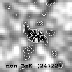
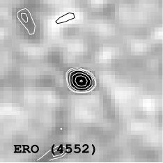
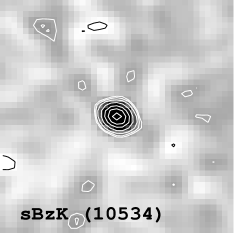
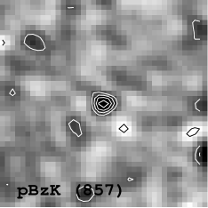
Figure 8: Postage-stamp images of the GMRT 610-MHz stacks for non-BzK, ERO, sBzK and pBzK samples. Contours for the non-BzK, ERO and sBzK are $-3,3,4,6,8$ then in steps of $+2\sigma$ while for pBzK they are $-2,2,3,4$ then in steps of $+1\sigma$. Stacks are the weighted-mean with $\pm 5\sigma$ pixels removed before stacking.

The spectral indices of the mJy and sub-mJy radio populations can give some clues to the nature of the radio emission. Above 1 mJy, steep-spectrum, radio-loud AGN dominate with $\alpha\sim-0.7$ (Bondi et al. 2007). Below 1 mJy, where the radio counts flatten and the new population emerges, the spectral index has been found to flatten (Ciliegi et al. 2003; Prandoni et al. 2006). Bondi et al. (2007) conducted a deep survey of the VVDS-VLA field with the GMRT and found that while the spectral index flattens from $\alpha=-0.67\pm 0.05$ at $S_{\rm 1,400}>500\,\mu$Jy to $-0.46\pm 0.03$ from $150<S_{\rm 1,400}<500\,\mu$Jy, it then steepens to $\alpha=-0.61\pm 0.04$ at fainter fluxes. They also find that early-type galaxies have flatter indices ($\alpha=-0.55\pm 0.04$) than late-type/starburst galaxies ($\alpha\sim-0.7$). Fomalont et al. (2006) compared 1,400- and 8,400-MHz maps and found that sources with $S_{\rm 1,400}<75\,\mu$Jy have steeper indices than brighter sources ($\alpha=-0.87\pm 0.05$, compared to $\alpha=-0.78\pm 0.04$). They claim that the AGN fraction is therefore decreasing below $100\,\mu$Jy. While the flattening of the spectral index between $200<S_{\rm 1,400}<1,000\,\mu{\rm Jy}$ was thought to be due to an increase in the contribution from flat-spectrum compact radio cores hosted by low-luminosity AGNs, with the subsequent steepening at $S_{\rm 1,400}<200\ \mu$Jy ascribed to an increasing dominance of starburst/late-type galaxies. Unfortunately, this observed steepening at sub-mJy fluxes is not yet a statistically robust phenomenon, due partly to the spectral index bias: a population selected at a high frequency is less likely to be found to have flat spectral indices if the low-frequency flux limit is higher than the high-frequency limit.

We will now investigate whether stacking the $K$-selected populations into radio maps at two frequencies can shed any light on the behaviour of the radio spectral index at $S_{\rm 1,400}<50\ \mu$Jy.

5.1.1 GMRT observations and stacking

For our second frequency, we employ a 610-MHz map taken with the Giant Metre-wave Radio Telescope (GMRT) near Pune, India. Data were obtained in the UDS field during 2006 February 03–06 and December 05–10, primarily to explore the spectral index of the radio emission from submm-selected galaxies, though a byproduct has been a thorough exploration of spectral indices of the faint background population (Ibar et al., in preparation). Typically, we were able to employ 27–28 of the 30 antennas that comprise the GMRT, observing a mosaic of three positions, arranged like the VLA mosaic. The total integration time in each field, after overheads, was around 12 hr. We recorded 128$\times$1.25-kHz channels every 16 s in the lower and upper sidebands (602 and 618 MHz, respectively), in each of two polarisations. Integrations of 40-min duration were interspersed with 5-min scans of the bright nearby calibrator, 0240$-$231, with scans of 3C 48 and 3C 147 for flux and bandpass calibration.

Calibration initially followed standard recipes within $\cal AIPS\/$. However, because of concerns that some baselines were picking up signal from local power lines, a raft of new measures were introduced to avoid detrimental effects on the resultant images. These are to be reported in detail in Ibar et al.

Imaging each of these datasets entailed mosaicing 37 facets, each 512${}^{2}\times$ 1.25²-arcsec² pixels, to cover the primary beam. A further 6–12 bright sources outside these central regions, identified in heavily tapered maps, were also imaged. Our aim was to obtain the best possible model of the sky. clean boxes were placed tightly around all radio sources for use in self-calibration, first in phase alone, then in amplitude and phase.

The final six mosaics, two for each pointing (upper and lower sidebands), were convolved to a common beam size, then knitted together using flatn. An appropriate correction was made for the shape of the primary beam and data beyond the quarter-power point of the primary beam were rejected. Data for each pointing and sideband were weighted according to individual noise levels. The final flatned image has a noise level of 57 $\mu$Jy beam^-1 — significantly higher than images of the Lockman Hole field during the same observing period. The reasons for this include the extra RFI suffered during day-time observing, the low declination of the UDS and the presence of several very bright radio emitters in the field.

The stacking was performed in the same way as for the 1,400-MHz map, except that the BWS correction is negligible for the GMRT’s narrow channels. Regions with $\sigma_{\rm 610MHz}\leq 120\,\mu$Jy were included in the stack. We calculated the correction for integrated flux and dirty-to-clean as we have for the 1,400-MHz data. The final correction value was found to be a factor $1.20\pm 0.15$. All spectral indices are quoted after making corrections at both frequencies.

Due to the noise being much higher in the GMRT data, only stacks of total populations could be made (not split as a function of redshift, $K$ mag, etc.). We also stacked sets of random positions into the GMRT map to check for systematics and we found that the means are consistent with zero. The medians are generally a little below the means and there is a possible $-0.1\ \mu$Jy offset, consistent with the median background removal applied to the map which would have resulted in negative patches around bright sources. We will not correct for this effect as it is negligible.

5.1.2 Spectral index results

The results of the stacking for the $K$-selected populations are listed in Table 3 and the postage-stamp images are shown in Fig. 8. It must be noted here that our spectral index measurements are the ratio of two ‘average’ quantities, flux at 610 MHz and flux at 1,400 MHz. As such, we cannot calculate the true average spectral index, as would be the case if samples of sources were detected at both wavelengths and their individual spectral index values averaged. It is possible that there are situations where this may bias our values of the spectral index, particularly if $\alpha$ is correlated with $S_{\rm 1,400}$ as seems to be suggested in the literature (Fomalont et al. 2006; c.f. Ibar et al. in preparation). We investigated this possibility using a simple Monte-Carlo simulation. We generated sources with a power-law distribution of $S_{1,400}$, following $dN=S^{-\gamma}\,dS$ and for each source we assigned a value of $\alpha$ between $-0.9$ and $0.0$. We provided the $\alpha$ values according to two models, one where $\alpha$ is random and another where $\alpha$ depends on $S_{1,400}$ as $\alpha=-0.9+0.5\log\,(1+$$S_{\rm 1,400}$$/50)$. Below 50 $\mu$Jy which we introduce an asymptote to $\alpha=-0.9$ as $S_{\rm 1,400}$ approaches zero. These choices reproduce the mean fluxes and values for $\alpha$ we find for our stacks. We then used the values of $S_{1,400}$ and $\alpha$ for each artificial source to calculate the value of $S_{610}$. The average spectral index in the simulation was then compared to the spectral index derived from the mean fluxes at both frequencies, as we have done in the stacks. The results showed that for input source counts with slopes $\gamma>1.5$, the bias on the spectral index derived from the stacking method is very small – a flattening of 0.01 in $\alpha$ for the model where $\alpha$ varies with $S_{1,400}$ and a steepening in $\alpha$ of 0.05 for the model where $\alpha$ is random. The slope of the 1,400-MHz differential counts at faint fluxes $\sim$30–75 $\mu$Jy is 2.0–2.5 (Fomalont et al. 2006; Biggs & Ivison 2006). If this holds at fainter fluxes, our method should not significantly bias the measured spectral indices; indeed, it probably gives values closer to the true spectral index than surveys which use detected sources.

The spectral indices are consistent, within the errors, across all the samples. The very faint flux regimes we are probing here are below any other work which has measured spectral indices. The average for the whole $K$-selected sample at ($z>0.2$) is $\alpha=-0.74\pm 0.03$. This is consistent with values for $\alpha$ in star-forming samples (Bondi et al. 2007; Ibar et al. in preparation) but is lower than the value found at faint fluxes by Fomalont et al. 2006. It may have been expected that pBZK galaxies would show a latter value for $\alpha$ then sBZK galaxies if radio-quiet AGN were the dominant contributors to the stacked radio flux. There is a hint that such a flattening is present but, with the current noise levels on the pBZK stack, this difference is not significant.

The corrections we have had to make for integrated flux versus peak flux mean that there are further systematic errors ($\sim\pm 0.15$) atop those quoted (which are from the stack statistics only). The GMRT beam is particularly unpleasant in the UDS field due to poor $(u,v)$ coverage, meaning the correction factor to clean-integrated flux density is more uncertain than that derived at 1,400 MHz, where it was clear that source size and positional errors were producing a broadening compared to the VLA beam. Although we can compare samples in our data in a consistent way and are confident that they are as similar or different as they appear, the exact value of the spectral index is rather sensitive to the corrections we are making. On the other hand, we are not hampered by the spectral index bias, as mentioned above, since we do not need to detect sources in both catalogues in order to measure the statistically averaged indices. Overall we would argue that this spectral index investigation is consistent with the hypothesis that star formation is the main contributor to the radio emission in these stacks as implied by Fomalont et al. (2006), Seymour et al. (2008) and Ibar et al. (in preparation).

5.2 Submm stacking of BzK galaxies

As another test of the reliability of the radio as a tracer of star formation, we compared it to the SFR from stacking the sBzK and pBzK samples into the submm map of the SXDF from the SHADES survey (Mortier et al. 2005; Coppin et al. 2006). Noise-weighted means and medians were calculated at the pixels corresponding to the positions of the $K$ galaxies. For the mean stacks, we excluded pixels with $\rm|S/N|\geq 5$. The submm beam is 14 arcsec and so the stacked pixel fluxes should represent the total flux for the $K$ galaxies. To check that there were no systematic effects, we examined the distribution of pixel signal-to-noise ratios (SNRs) in the map, as seen in figure 9 of Mortier et al. (2005). The mean SNR of 0.04 and variance of 1.15, which for a mean noise level in the map of $2.2\,\rm{mJy\,beam^{-1}}$, are consistent with zero.

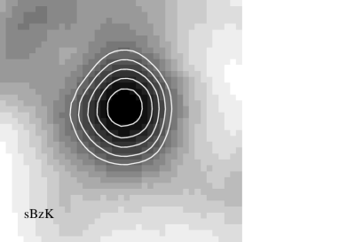
Figure 9: Stacked image of the 850$\mu$m SHADES map at the locations of the sBzK sources (1421 in total, excluding the one detection at $>5\sigma$). Contours are at $5,6,7,8,9\,\sigma$ and the image is $41\times 41$-arcsec.

The resulting 850-$\mu$m stacked flux was extrapolated to $L_{\rm FIR}$ using a modified black-body SED ($\nu^{\beta}\,B(\nu,T)$) with a dust emissivity index $\beta=1.5$ and dust temperatures of 30 k and 35 k. Two reasonable temperatures were chosen to provide an indication of the effect temperature has on the estimate of $L_{\rm FIR}$. $L_{\rm FIR}$ was then converted to an SFR using the relationship given by Kennicutt (1998), where ${\rm SFR}(M_{\odot}\,\rm{yr^{-1}})=1.7\times 10^{-10}\,L_{\rm FIR}/L_{\odot}$. Only one pixel in the sBzK galaxy stack was at $>$5$\sigma$ and so we are confident that the noise-weighted mean is the most efficient estimator of the average properties of the submm stack. The results are presented in Table 4 and show that the radio- and submm-derived SFRs are in good agreement, within the uncertainties of the calibrations. This is another reassurance that the radio emission from the sBzK galaxy sample is not dominated by AGN. The overall detection of sBzK galaxies is in good agreement with that of Takagi et al. (2007) who found a mean $S_{\rm 850\mu m}=0.53\pm 0.19$ mJy, though with far fewer sources (112 compared to 1,421). It is interesting to note that the 850-$\mu$m stacked flux density also correlates with absolute $K$ mag.

The total pBzK sample was not detected and the small number of sources overlapping the submm map means that the upper limit is not sensitive enough to constrain the nature of the radio emission. The upper limit to the submm-derived SFR is consistent with that determined through radio stacking. On splitting the pBzK galaxies into two redshift bins, $z<1.4$ and $z>1.4$, we see a 2.6-$\sigma$ detection in the submm band in the low-redshift bin. Although not formally significant, this suggests that the $z<1.4$ pBzK galaxies are a strongly star-forming sample, and their submm emission is consistent with radio emission powered by star formation. At $z>1.4$, there is no submm emission, but again the upper limits are not deep enough to constrain the origin of the radio emission.

Another way to look at the stacked submm and radio fluxes is in terms of the FIR/radio correlation. The FIR/radio ratio is defined as

$$q=\log[\frac{S_{\rm FIR}/3.75\times 10^{12}\,\rm Hz}{S_{\rm rad}}]$$

where $S_{\rm FIR}$ is given by Helou et al. (1985) as

$$S_{\rm FIR}=1.4\times 10^{-14}(2.58\,S_{60}+S_{100})\,{\rm Wm^{-2}}$$

where $S_{60}$ and $S_{100}$ are the 60- and 100-$\mu$m flux densities in Jy. $S_{\rm rad}$ is the radio flux in units of ${\rm Wm^{-2}Hz^{-1}}$ and several different frequencies are used in the literature.

Radio-bright AGN (such as core-dominated Seyferts) have lower $q$ values than samples composed purely of SFGs. We have calculated $q$ for our sample of sBzK galaxies under the two temperature assumptions used above (since we do not measure directly the rest-frame 60- and 100-$\mu$m part of the spectrum). The results are summarised in Table 5. Unfortunately, our lack of knowledge of the dust temperatures in the sBzK galaxies limits the usefulness of this approach. For a dust SED with $T=30$ k, we find $q$ is low compared to the star-forming FIR/radio relation, and more similar to the values found in Seyfert samples; for a dust SED with $T=35$ k, we find $q$ to be entirely consistent with star-forming values. The average temperature of IRAS-bright galaxies in the local Universe is $T\sim 35$ k (Dunne et al. 2000), and galaxies containing an AGN would usually tend to have hotter dust than those without – due to extra heating of dust near the nuclear regions. The $q$ values we find are only similar to those of Seyferts for the coldest dust temperature assumptions, if we use a dust temperature more appropriate for AGN dominated galaxies (e.g. $T=50$ k; Kuraszkiewicz et al. 2003) the we see from Table 5 that the $q$ values are then inconsistent with those derived for AGN. This is further evidence that star formation is dominating the radio emission of our sBzK sample. Further investigation of the FIR/radio relationship will be possible with forthcoming Herschel observations which will directly measure the temperature of the dust out to high redshift.

Table 4: Results of stacking BzK galaxies into the SHADES 850-$\mu$m SXDF map.

Sample	$K_{\rm abs}$(Vega)	$\langle z\rangle$	N	$\bar{S}_{\rm 850\mu m}$	$\rm SFR^{sub}_{35K}$	$\rm SFR^{sub}_{30K}$	$\rm SFR^{rad}_{C}$	$\rm SFR^{rad}_{B}$
				(mJy)	($\rm M_{\odot}\,yr^{-1}$)	($\rm M_{\odot}\,yr^{-1}$)	($\rm M_{\odot}\,yr^{-1}$)	($\rm M_{\odot}\,yr^{-1}$)
sBzK	all	1.56	1,421	$0.53\pm 0.06$	$156.3\pm 16.6$	$80.2\pm 8.9$	$153.6\pm 6.7$	$70.6\pm 3.1$
	$-(21.5-23.5)$	1.41	187	$0.17\pm 0.16$	$<128$	$<65$	$30\pm 12$	$14\pm 6$
	$-(23.5-24.5)$	1.54	509	$0.17\pm 0.10$	$<83$	$<42$	$92\pm 10$	$42\pm 5$
	$-(24.5-25.5)$	1.63	442	$0.76\pm 0.10$	$230\pm 31$	$119\pm 16$	$226\pm 11$	$104\pm 5$
	$-(25.5-26.6)$	1.74	212	$1.19\pm 0.15$	$380\pm 46$	$197\pm 24$	$485\pm 27$	$223\pm 12$
	$-(26.5-27.5)$	2.16	33	$1.60\pm 0.37$	$618\pm 141$	$329\pm 75$	$1267\pm 175$	$583\pm 80$
pBzK	all	1.53	147	$0.22\pm 0.18$	$<158$	$<81$	$131\pm 19$	$61\pm 9$
pBzK $z<1.4$	all	1.28	46	$0.89\pm 0.34$	$219\pm 84$	$111\pm 42$	$158\pm 19$	$73\pm 9$
pBzK $z>1.4$	all	1.66	101	$-0.05\pm 0.22$	$<200$	$<103$	$105\pm 31$	$48\pm 14$

Table 5: Comparison of FIR/radio ratios for sBzK and samples from the literature.

Ref.	$q_{\rm SF}$	$q_{\rm AGN}$	$q_{\rm sBzK}$	$q_{\rm sBzK}$	$q_{\rm sBzK}$
			(30K)	(35K)	(50K)
A	$2.83\pm 0.03$	$2.55\pm 0.14$	$2.53\pm 0.05$	$2.82\pm 0.05$	$3.36\pm 0.05$
B	$2.48\pm 0.10$	$1.87\pm 0.08$	$2.18\pm 0.05$	$2.48\pm 0.05$	$3.02\pm 0.05$
C	$2.300\pm 0.003$	$2.00\pm 0.04$	$2.00\pm 0.05$	$2.29\pm 0.05$	$2.82\pm 0.05$

6 Discussion: the SFRs of $K$-selected galaxies

We now split the samples into bins of redshift and stellar mass ($M_{\rm stellar}$), or absolute rest-frame $K$ mag. The rest-frame $K$ mags are calculated with the photometric redshifts using the best-fitting SED template. These are then converted into $M_{\rm stellar}$ using the relationship given by the Millennium simulation (de Lucia et al. 2006) in the manner employed by Serjeant et al. (2008) which is effectively using a Salpeter IMF. This is a redshift-dependent conversion which agrees with observational data from the Munich Near-IR Cluster Survey (MUNICS – Drory et al. 2004). There are, of course, uncertainties in moving between $K$ and $M_{\rm stellar}$; the scatter in the relationship used here is of order 0.2-0.3 dex at a given redshift. A more careful measurement will be possible in the future using the results of the Spitzer Legacy survey of the UDS, in particular the 3.6–8-$\mu$m data. We have checked that using $M_{\rm stellar}$ rather than the simpler absolute $K$ mag does not change the trends discussed in this section. We use $M_{\rm stellar}$ as this is more directly comparable to other work in the literature.

6.1 Star-formation history

To begin with, we look at the SFRD as a function of redshift for our full sample (i.e. ‘All galaxies’ from Section 3.1). The sample was divided into a number of redshift bins and the median SFR for each bin calculated. The volume contained within each bin was calculated using the effective survey area (UDS/SuprimeCam/VLA overlap field, excluding regions around bright stars and with $\sigma_{\rm 1,400}\leq 20\,\mu$Jy) which is 1311.1 arcmin². The space density is the number of sources meeting the selection criteria in that redshift bin divided by the volume in the bin. The space density is corrected for the 80 percent completeness of the $K$-sample in the magnitude range $22.5<K\leq 23.0$ by finding the number of galaxies within each redshift bin in this magnitude range, multiplying that number by 1.2 and adding it to the number of galaxies in that redshift bin at $K\leq 22.5$. These corrections are small and range from 1.04 at low redshift to 1.13 at $z>3.0$. The SFRD is estimated by multiplying the space density by the median stacked SFR for each redshift bin. The results are shown in Fig. 11 for both methods of estimating the SFR. The errors on the points are the sum in quadrature of the error on the median SFR for a bin, the Poisson $1/\sqrt{N}$ contribution and cosmic variance errors, derived from fig. 2 in Somerville et al. (2004). Plotted in grey are the points from the compilation of Hopkins & Beacom (2006, hereafter HB06). Our radio-derived SFRs do not come from a flux-limited sample and thus can, in principle, span the full radio luminosity function (LF) at all redshifts. However, the $K$-selected sample we are stacking does lose lower $K$ luminosity sources at higher redshifts. If the radio-derived SFR and $K$-band luminosity are correlated then we will have an effective ‘luminosity limit’ to our radio stacks, as a function of redshift, which will mean that we will be missing some fraction of the SFRD at higher redshifts. We have checked this by stacking in bins of absolute $K$ mag ($M_{K}$) and the results are shown in Fig. 10. We stacked in two redshift bins ($z<1$ and $z>1$) to minimise any redshift-dependent trends. The fits in both cases show ${\rm SFR}\propto L_{K}^{1.01-1.05}$ which, within the uncertainties, is consistent with a linear relationship.

We will now attempt to correct for the fraction of the radio luminosity density lost from the faint end of the $K$-band LF. The deepest wide-area study of the evolution of the $K$-band LF is provided by the UDS (Cirasuolo et al. 2008) who present Schechter function fits as a function of redshift. The integrated luminosity in $K$ from infinity to some fixed lower luminosity ($L$) is given by:

$$\rho_{L}(K)=\phi_{\ast}L_{\ast}\Gamma(\alpha+2,L/L_{\ast})$$

where $\phi_{\ast}$ is the normalisation, $L_{\ast}$ is the characteristic luminosity in $K$, $\alpha$ is the faint-end slope and $\Gamma(\alpha+2,L/L_{\ast})$ is the incomplete Gamma function.

The correction we want to make ($C$) for each redshift bin is the ratio of $\rho_{L}(K)$ integrated to the lowest observed luminosity at that redshift – the cut-off luminosity ($L_{\rm cut}$), to $\rho_{L}(K)$ integrated to $L_{\rm min}$, the lowest observed luminosity at $z=0$. We used the evolving $L_{\ast}$ from Cirasuolo et al. (2008), with a fixed faint-end slope and calculated $L_{\rm cut}$ for each redshift bin. Thus

$$C=\frac{\rho_{L}(K)_{\rm tot}}{\rho_{L}(K)_{\rm obs}}=\frac{\Gamma(\alpha+2,L_{\rm min}/L_{\ast})}{\Gamma(\alpha+2,L_{\rm cut}/L_{\ast})}$$

The radio SFRD points were corrected by the factor $C$ and are shown as solid circles on Fig. 11. The uncorrected values are also shown as open diamonds in Fig. 11 for comparison.

Figure 10: Radio-derived SFR versus absolute $K$ mag for $z<1$ (open diamonds) and $z>1$ (filled diamonds). The best fits are shown and are consistent with ${\rm SFR}\propto L_{\rm K}$.

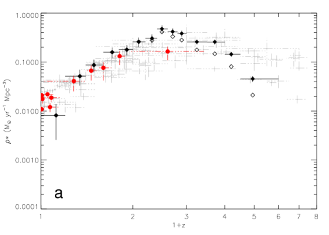
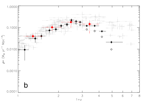
Figure 11: Radio-derived star-formation histories using: (a) the SFR relationship of Condon (1992); (b) that of Bell (2003). The faint points are the compilation of HB06 normalised to a Salpeter IMF. Red circles in (a) show literature values (Condon 1989; Condon et al. 2002; Haarsma et al. 2000; Machalski & Godlowski 2000; Sadler et al. 2002; Mauch & Sadler 2007) derived from 1,400-MHz data using the Condon (1992) conversion. Red circles in (b) show the values from Seymour et al. (2008) at 1,400 MHz for the Bell (2003) SFR conversion, converted to a Salpeter IMF. All the SFRD points are corrected for the detection incompleteness, filled symbols are also corrected for LF incompleteness using the UDS LF from Cirasuolo et al. (2008) while open symbols show LF uncorrected points. Out to $z\sim 2$, the radio-derived points using both SFR relations are in good agreement with literature values, both in the radio and other optical wavelengths. The radio-derived SFRD then declines more steeply than the points from HB06.

The radio-derived SFRD is consistent with the multi-wavelength compilation of HB06 out to $z\sim 2$. After this, the radio-derived points appear to drop more steeply than the other data, even after correction for the missing faint end part of the $K$-band LF. This is the highest redshift study of star formation in the radio to date and it is not clear why the shape of the radio SFRD should be different to that derived in the optical waveband. One possibility is that the radio breaks down as a tracer of SFR at high redshift. Carilli & Yun (1999) suggest that radio emission could be quenched at high redshift by inverse Compton scattering from the microwave background, but it is believed that this should only be a serious effect at $z>6$. So far, no evolution has been observed in the radio/FIR correlation out to $z\sim 3$ (Kovacs et al. 2006; Ibar et al. 2008) but these studies focus on samples with much higher $L_{\rm 1,400}$ and $L_{\rm FIR}$. Our LF corrections may also be underestimated if the faint end slope of the $K$-band LF undergoes evolution with redshift. The optical/UV points at $z>2$ are also subject to substantial correction for the effects of dust, which may not be appropriate at these redshifts. Thus, we have no reason to suspect that the radio-derived values are less valid than those derived at shorter wavelengths, and some reason to suppose that they are rather more trustworthy.

We can also compare the radio-derived SFRD determined using the two SFR relationships discussed earlier. Fig. 11a shows the conversion of 1,400-MHz luminosity to SFR from Condon (1992) while Fig. 11b shows that of Bell (2003). Both SFR calibration methods straddle the points from HB06, with Condon’s a little high, and Bell’s a little low. In Fig. 11, we also highlight as red circles the literature points derived from other 1,400-MHz surveys. The stacked points are in very good agreement with these until $z\sim 1-2$. At the highest redshifts, the literature radio studies are making very large corrections for the LF (which is not measured at radio wavelengths at these distances) whereas our corrections are more modest and are based on measured $K$-band LFs. For comparison, our maximum LF correction is a factor 2$\times$ at $z\sim 4$, compared to a correction of 6$\times$ at $z\sim 2.5$ for Seymour et al. (2008).

The lowest redshift point, at $z<0.2$, has been corrected (to integrated and for clean-to-dirty) by a factor 2.61, as described in §3.2. Without this differential correction for the lowest redshift bin, this point would be very low compared to the literature points from HB06. It is still noticeably lower than the higher redshift points in Fig. 11a based on the Condon SFR conversion, though using the Bell SFR gives better agreement. Given our reliance on photometric redshifts, where the magnitude of $\delta z/z$ is of order unity for $z<0.2$, it is possible that uncertainties in redshift are producing this decrement. Until more spectroscopic redshifts are available to help calibrate the photometric redshifts, we cannot address this issue adequately and so will not discuss sources at $z<0.2$ further.

The general agreement between the two SFR estimators and the literature work further supports the mounting evidence that AGN are not strongly contributing to the globally-averaged radio emission of these stacked samples. Overall, at this point, we feel there is nothing to choose between the two SFR conversions and so will continue to use both in the following section.

6.2 Specific star-formation rates

We can also look at the average SFR per unit stellar mass, defined as the SSFR, as a function of stellar mass and redshift. SSFR is often used as a measure of the star-formation efficiency of a galaxy, since it provides information about the fraction of a galaxy’s mass which could be converted into stars in a given time. A higher SSFR means a galaxy will increase its mass by a greater fraction in a given time than a lower SSFR.

The results for the full $K$-selected sample are shown in Fig. 12, where Fig. 12a uses Condon’s SFR and Fig. 12b uses Bell’s SFR. We see a strong trend of increasing SSFR with redshift for all bins of stellar mass. There is no difference in the evolution of SSFR with redshift for different mass bins out to $z\sim 2$, after which the high-mass bins tend to flatten off compared to the low-mass bins. There is also a trend that the least massive galaxies at any redshift have the highest SSFR (becoming more pronounced with increasing redshift). The difference between Bell’s and Condon’s SFRs are clear in two ways. First, the SSFRs are higher overall for the Condon SFR estimator and, second, the trends in the lowest redshift bin are significantly different. This is because the low-redshift bin contains a number of mass bins where the radio luminosity is below $L_{c}$ in the Bell (2003) relationship. As a result, the Bell (2003) conversion boosts these low $L_{\rm 1,400}$ points to account for his finding that low-luminosity galaxies are deficient in non-thermal radio flux for a given SFR. Fig. 12b therefore shows a trend for the lowest mass galaxies to have the highest SSFR in the lowest redshift bin, whereas Fig. 12a (Condon SFR) does not.

A large volume of literature on SSFR has been produced since recent advances in deriving robust stellar masses for large galaxy samples through deep and wide $K$-band and Spitzer imaging (Feulner et al. 2005, 2007; Caputi et al. 2006; Zheng et al. 2007; Daddi et al. 2007; Elbaz et al. 2007; Iglesias-Paramo et al. 2007; Perez-Gonzalez et al. 2007; Salim et al. 2007; Martin et al. 2007; Buat et al. 2007). These investigations all report two similar trends, though the exact values tend to differ depending on the conversions to $M_{\rm stellar}$ and the method used to determine SFR. Firstly, they find that SSFR increases with redshift for all masses of galaxy – high-redshift galaxies were forming stars not only at a higher absolute rate than low-redshift galaxies, but also at a higher rate compared to their stellar mass. Secondly, SSFR studies in the literature also show that the highest SSFR at any given redshift is displayed by the lowest mass galaxies, with many studies finding that SSFR has dropped more rapidly since $z\sim 2$ in the most massive galaxies (Feulner et al. 2005; Perez-Gonzalez et al. 2007). Many authors have claimed that this difference in the SSFR behaviour at high and low masses is akin to differential evolution – the so-called ‘downsizing’, discovered originally via a $K<22$ ($B<24.4,I<23$) survey and described as a ‘smooth decrease in the characteristic luminosity of galaxies dominated by star formation’ (Cowie et al. 1996).

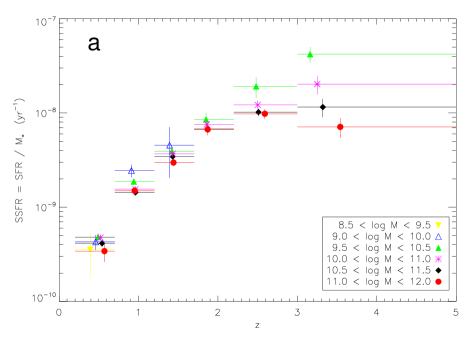
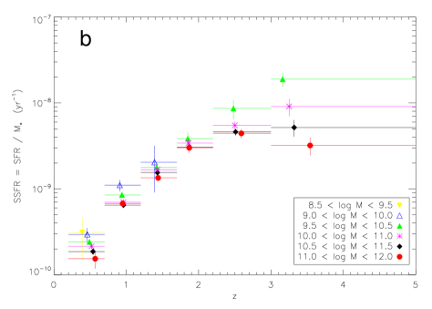
Figure 12: SSFR (SFR/$M_{\rm stellar}$) as a function of redshift for the UDS galaxies. Error bars are based on the 1$\sigma$ confidence interval on SSFR, as measured directly from the distribution of values in the stack, with no account taken of possible systematics from determination of $M_{\rm stellar}$ via $K$ mag. (a) shows SSFR using the Condon SFR conversion and (b) is the Bell SFR conversion. Various symbols represent different $M_{\rm stellar}$ bins as explained in the legend.

a) SSFR using the Condon SFR conversion.

b) SSFR using the Bell SFR conversion.

Figure 13: SSFR as a function of stellar mass for various redshift bins. The dynamic range of the sub-panels is the same, so slopes are directly comparable. Masses plotted are the median mass from the bins in Fig. 12. The panels for $z\sim 0.5$, $z\sim 1$ and $z\sim 2$ are compared to the results of Brinchmann et al.  (2004), Elbaz et al. (2007) and Daddi et al. (2007). The solid line shows the fit to our data while dashed lines show fits from the literature. The dash-dot line in the $z\sim 1$ panel is the fit without the lowest-mass bin. This is in keeping with the mass range fitted by Elbaz et al. (2007). The slopes are consistent at $z=1-2$, but the normalisation is different due to the different SFR indicators and $M_{\rm stellar}$ estimates. At $z=0.5$, the slope is intermediate between that of Brinchmann et al. (2004) at $z=0$ and Elbaz et al. (2007) at $z=1$.

We will now make a detailed comparison between our results and those in the literature and discuss possible reasons for the differences.

Fig. 13 shows in more detail the relationship between SSFR and $M_{\rm stellar}$. Fig. 13a uses the Condon SFR and Fig. 13b uses the Bell SFR. From this we can notice two things. First, most panels show a weak relationship between SSFR and $M_{\rm stellar}$, where the steepness of the correlation appears to increase with redshift. Second, we note the difference in appearance of the lowest redshift bin when using the different SFR conversions. With the Condon SFR, there is no apparent trend while for the Bell SFR, there is a significant correlation. Given the number of studies finding such a relationship at low redshift, and that we also find a similar trend at higher redshifts, we feel that this is tentative evidence supporting the Bell SFR estimation.

We have over-plotted comparisons with other literature where available. The studies by Daddi et al. (2007) of BzK galaxies at $z=2$, and by Elbaz et al. (2007) of sources at $z=1$ selected using 24-$\mu$m data in the Great Observatories Origins Deep Survey (GOODS), are over-plotted on the $z=0.95$ and $z=1.85$ panels of Fig. 13. They find a correlation between SFR and $M_{\rm stellar}$ which is almost linear (SFR $\propto M_{\rm stellar}^{0.9}$) leading to a shallow dependence of SSFR on mass. The study of $z=0$ galaxies from the SDSS by Brinchmann et al. (2004) finds a shallower slope of ${\rm SFR}\propto M_{\rm stellar}^{0.77}$. The Brinchmann et al. trend is overplotted at $z=0.5$ to show that the slope of the relationship we find is intermediate between that at $z=0$ and $z=1$.

The rather weak trends of SSFR versus $M_{\rm stellar}$ found here are at some odds with other findings in the literature. Some studies find that the differences in SSFR at $z=0.6-1$ over the mass range $8.5<\log\,M_{\rm stellar}<11.5$ to be a factor $10-32$ compared to our differences of a factor $1.6-2$ (Feulner et al. 2005; Caputi et al. 2006; Zheng et al. 2007; Pérez-González et al. 2007). In our highest redshift bins ($z>2$) we can see a steepening of the relationship between SSFR and $M_{\rm stellar}$, however these are not well-fitted by a power law. Extrapolating the linear portion of the $z=3.3$ panel, we find that the change in SSFR over the range $8.5<\log\,M_{\rm stellar}<11.5$ at $z\sim 3.3$ is a factor $\sim 25$ – closer to the values seen at lower redshift in the other studies.

Most of the surveys reporting these steeper trends have two things in common. First, they are selected in the optical and use $K$ or Spitzer data to estimate $M_{\rm stellar}$. Second, they rely on detections of galaxies in one or more bands, from which the SFR is then directly inferred (e.g. UV, 24 $\mu$m). The rest-frame UV is the most sensitive to low levels of SFR and thus the method by which most of the low-mass bins have been determined. For a low-mass galaxy with a low SSFR to be part of such a sample, the sensitivity to SFR in the survey must be very high and there is therefore a potent selection bias: low-mass galaxies with higher-than-average SSFRs are included preferentially in such samples. This was noted by Feulner et al. (2007), who investigated the effects of survey wavelength on the slope of the SSFR vs $M_{\rm stellar}$ relation at various redshifts. They found that $B$-band surveys select via SFR, effectively, while $K$-band surveys select via stellar mass (for $z<1.5$, at least). $B$-band selection produces greater correlation between SSFR and $M_{\rm stellar}$. This selection band bias most strongly affects low-mass galaxies. Elbaz et al. (2007) and Zheng et al. (2007) also noted that optical selection for spectroscopic completeness leads to a loss of red (low-SFR) low-mass galaxies, pushing up the apparent SSFR in the lowest-mass bins, which suggests at least one pragmatic argument in favour of using high-quality photometric redshifts.

Our sample is based on selection via an extremely deep $K$-band survey (where selection is not strongly dependent on current SFR at $z<1.5$) and the current SFR is determined by radio stacking (rather than via a flux-limited radio sample). The weak dependence of SSFR on $M_{\rm stellar}$ at $z<2$ found here – and the similar evolution of SSFR with redshift across all masses – could be explained by our less biased selection. At $z>2$, $K$ is shifting into the rest-frame optical, making our selection more SFR-based than $M_{\rm stellar}$-based. As predicted, this causes a stronger apparent trend of SSFR with $M_{\rm stellar}$ because high-SSFR objects are preferentially selected near the limit of the survey.

In summary, many independent studies find similar trends, with SSFR increasing with redshift and decreasing with stellar mass. However, the strength of these relationships varies considerably and is likely to be due to a complicated combination of sample-selection criteria, particularly wavelength and depth. Many authors make strong statements about downsizing, based on the evolution of SSFR with redshift in different stellar mass bins, and on the oft-strong correlation of SSFR with stellar mass. We would urge caution before over-interpreting this type of plot as it is influenced strongly by selection biases. Given that our exploration of SFR versus absolute $K$ mag produced a linear correlation, with $\rm SFR\propto L_{K}^{1.01-1.05}$, it is the conversion of $K$ mag to stellar mass which introduces the slight non-linearity in SFR versus $M_{\rm stellar}$ ($\rm SFR\propto M_{\rm stellar}^{0.9}$). This, in turn, produces the shallow observed dependence of SSFR on $M_{\rm stellar}$. Thus, the conversion to stellar mass can also introduce systematic effects, producing trends in SSFR with $M_{\rm stellar}$.

The upcoming addition of extremely deep $U$, $H$ and 3.6–24-$\mu$m Spitzer imaging, as well as several thousand more spectroscopic redshifts, the stellar masses and redshifts of the UDS sample will improve markedly. At that time, it will be interesting to test whether these trends remain.

6.3 Specific star-formation rates in BzK galaxies

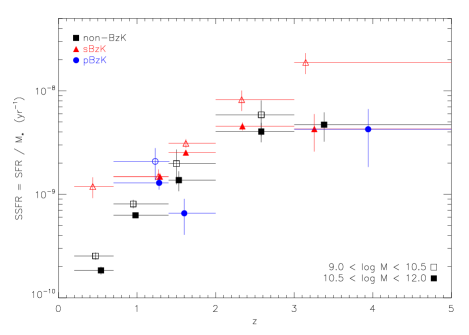
Figure 14: SSFR using the Bell’s SFR conversion with redshift and mass for sBzk (red triangles), pBzK (blue circles) and non-BzK galaxies (black squares). Objects with log $M_{\rm stellar}=9.0-10.5$ ($10.5-12.0$) are denoted by open (filled) symbols.

We have further split the samples of sBzK, pBzK and non-BzK galaxies into bins of redshift and stellar mass to investigate their SSFR trends. This is shown in Fig. 14 with different colours and symbols denoting the different samples and open and filled symbols used to denote the mass ranges. Here we see a similar trend to Fig. 12, with SSFR increasing with redshift. The sBzK galaxies tend to have slightly higher SSFRs for a given mass than the non-BzK galaxies, consistent with the idea that they are a strongly star-forming population. In the lowest-redshift bin ($0.2<z<0.7$), sBzK galaxies are forming stars more actively than non-BzK galaxies in the same redshift and mass range. The subset of sBzK galaxies at low redshift have very blue colours and are fainter in $K$ than non-BzK galaxies in the same redshift interval. Kolmogorov-Smirnov (K-S) tests show that the radio flux densities, SSFRs and $K$ mag distributions are significantly different from the main low-redshift non-BzK galaxy sample at probabilities of $0.015,\ 1.3\times 10^{-9}$ and $9.2\times 10^{-13}$ respectively. The flat, blue spectra of these galaxies makes it very difficult to assign accurate photometric redshifts and, as they represent only a small fraction of the galaxies at this redshift ($\sim$1–2 per cent) they could be photometric-redshift outliers. If their redshifts were increased to $z\sim 1-1.4$, their SSFRs would not be remarkable compared to other galaxies at this redshift. If they truly do lie at low redshift, they represent a population of low-mass, highly star-forming galaxies, quite unlike the general low-redshift population. Confirmation of their nature must await spectroscopy.

The pBzK galaxies behave quite differently. Their SSFR drops from $0.7<z<1.4$ to $1.4<z<2.0$ and then appears to be consistent again with the other samples at very high redshifts. We have already noted changes in pBzK properties at $z=1.3-1.4$ from their radio spectral indices (§5.1), the decrease in their radio flux density and the suggestion of a similar decrease in their submm flux density. This argues that the BzK diagram alone is not discriminating effectively between passive and star-forming galaxies – accurate redshifts are also required. The persistent (but lower level) radio flux density at $z>1.4$ could be due either to low-level SFG contamination or to radio-quiet AGN activity. The radio spectral indices and submm stacking also suggest a change in the dominant pBzK population at $z\sim 1.4$, but our submm and 610-MHz observations are not deep enough to allow us to conclude which of the above scenarios is responsible for the low-level 1,400-MHz emission at $z>1.4$.

Future analysis of the larger SHADES 1.1-mm AzTEC image, newly acquired Spitzer data, alongside the zUDS spectroscopic programme, should determine the true nature of pBzK galaxies.

7 Conclusions

We have stacked several $K$-selected populations into a deep 1,400-MHz mosaic in order to investigate their star-formation history. There is much dispute over the relative contribution from star formation and AGN to the radio populations at sub-mJy levels and our knowledge is almost non-existent at flux levels below those where individual galaxies are usually detected ($<$100 $\mu$Jy). We certainly cannot distinguish unambiguously between star-formation- and AGN-related emission. However, their spectral indices, submm flux densities and the good agreement between SFRDs derived in the radio and that determined at other wavelengths argues that radio-quiet AGN do not make an important contribution to the average radio properties of our $K$-selected galaxies at these flux densities (5–20$\,\mu$Jy).

We find a strong relationship between stacked radio flux density and apparent $K$ mag. We also find SFR to be a strong and almost linear function of absolute $K$ mag and stellar mass.

Both sBzK and pBzK galaxies are detected robustly in the radio stack. The stacked radio flux density of the sBzK galaxies is roughly constant with redshift, inferring a strong evolution in SFR.

Our photometric redshifts suggest that a significant fraction ($\sim$30–40 per cent) of galaxies occupying the sBzK and pBzK regions of the BzK diagram lie at $z<1.4$. The similarity between sBzK and $z<1.4$ pBzK galaxies – in terms of their radio- and submm-derived SFR and SSFR – leads us to suggest that the BzK diagram alone is not sufficient to select passive high-redshift galaxies. Only pBzK galaxies at $z>1.4$ seem consistent with this designation, those at $z<1.4$ are likely to be star forming galaxies similar in nature to sBzK.

The pBzK galaxies suffer a dramatic reduction in radio flux density at $z>1.4$. Their weak radio flux density at $z>1.4$ suggests either a persistent, low-level of contamination by SFGs, or that the radio emission for these objects is powered by radio-quiet AGN. Deeper 610-MHz and submm data are required to determine which is the case.

The variation of radio-derived SFR density with redshift agrees well with that determined at other wavelengths, for $z=0.2-2.0$. This suggests that the contribution from AGN-related radio emission is small. At $z\geq 2$, the radio-derived SFR density declines due to our inability to fully sample the $K$-band luminosity function at these redshifts. After correcting for this, using the evolving $K$-band UDS LFs, we still see a downturn in the radio-derived SFRD at high redshifts which is not apparent in the other multi-wavelength data. The reason for this is not clear but we suggest three possibilities: (a) a changing slope with redshift for the $K$-band LF, which would mean our LF corrections have been underestimated; (b) dust corrections to the optical/UV data are too high; (c) the radio emission is not tracing star formation efficiently at high redshift, possibly due to evolution of the magnetic field properties or a change in the mode of star formation.

We find that the SSFR (SFR/$M_{\rm stellar}$) is only weakly dependent on stellar mass, with SSFR decreasing as $M_{\rm stellar}$ increases. The observed correlation of SSFR with stellar mass is consistent with the shallower determinations in the literature, such as Daddi et al. (2007) at $z\sim 2$ and Elbaz et al. (2007) at $z\sim 1$. It is much less steep than many optical-/UV-based studies and we argue that these differences are largely due to selection biases present in UV- and optically-selected samples. We also find a very strong trend of increasing SSFR with redshift, stronger than reported elsewhere, with a flattening at $z\mathrel{\raise 1.50696pt\hbox{$\scriptstyle>$}\kern-6.00006pt\lower 1.72218pt\hbox{{$\scriptstyle\sim$}}}2$. This is also where the difference between high- and low-mass bins becomes greatest and where $K$ begins to sample the rest-frame optical waveband, meaning that sample selection becomes more influenced by star formation and less by stellar mass.

Comparing the radio-derived SFR conversions from Bell (2003) and Condon (1992), the former provides a better match to the observed trends in SSFR versus stellar mass in the lowest mass bins, and also in reproducing the low-redshift SFRD seen in other wavebands.

In summary, the UDS has produced a statistically powerful sample of $K$-selected galaxies, including several thousand selected by colour to lie at high redshift. Stacking these samples into a deep 1,400-MHz radio image has enabled us to determine their radio properties at flux densities an order of magnitude fainter than has previously been possible with flux-limited radio surveys. The pseudo-stellar-mass selection achieved in the $K$ band – combined with a probe of star formation which is not limited to the rarest, brightest sources – has allowed us to follow the SFRD out to $z\sim 4$ and to investigate the evolution of SSFR in galaxies with redshift in a relatively unbiased way.

References

- [1] Bell E.F., 2003, ApJ, 586, 794
- [2] Bertin E., Arnouts S., 1996, A&A, 117, 393
- [3] Biggs A.D., Ivison R.J., 2006, MNRAS, 371, 963
- [4] Bolzonella M., Miralles J.-M., Pelló R., 2000, A&A, 363, 476
- [5] Bondi M. et al., 2007, A&A, 519, 527
- [6] Brinchmann J., Charlot S., White S. D. M., Tremonti C., Kauffmann G., Heckman T., Brinkmann J., 2004, MNRAS, 351, 1151
- [7] Bruzual G., Charlot S., 2003, MNRAS, 344, 1000
- [8] Buat V. et al., 2007, ApJS, 173, 404
- [9] Calzetti D., Armus L., Bohlin R.C., Kinney A.L., Koornneef J., Storchi-Bergmann T., 2000, ApJ, 533, 682
- [10] Caputi K.I., McClure R.J., Dunlop J.S., Cirasuolo M., Schael A.M., 2006a, MNRAS, 366, 609
- [11] Caputi K.I. et al., 2006b, ApJ, 637, 727
- [12] Carilli C.L., Yun M.S., 1999, ApJ, 513, L13
- [13] Casali M. et al. 2007, A&A, 467, 777
- [14] Ciliegi P., Zamorani G., Hasinger G., Lehmann I., Szokoly G., Wilson G., 2003, A&A, 398, 901
- [15] Cirasuolo M. et al., 2008, MNRAS, in press (arXiv:0804.3471)
- [16] Clewley L., Jarvis M.J., 2004, MNRAS, 352, 909
- [17] Coleman G.D., Wu C.-C., Weeman D.W., 1980, ApJS, 43, 393
- [18] Condon J.J., 1984, ApJ, 287. 461
- [19] Condon J.J., 1989, ApJ, 338, 13
- [20] Condon J.J., 1992, ARA&A, 315, 575
- [21] Condon J.J., Cotton W.D., Broderick J.J., 2002, ApJ, 124, 675
- [22] Coppin K. et al., 2006, MNRAS, 372, 1621
- [23] Corbett E.A. et al., 2003, ApJ, 583, 670
- [24] Cowie L.L., Songaila A., Hu E.M., Cohen J.G., 1996, AJ, 112, 839
- [25] Daddi E. et al., 2004, ApJ, 617, 746
- [26] Daddi E. et al., 2005, ApJ, 631, L13
- [27] Daddi E. et al., 2007, ApJ, 670, 156
- [28] de Lucia G., Springel V., White S.D., Croton D., Kauffmann G., 2006, MNRAS, 366, 499
- [29] van Dokkum P.G. et al., 2004, ApJ, 611, 703
- [30] Drory N., Bender R., Feulner G., Hopp U., Maraston C., Snigula J., Hill G.J., 2004, ApJ, 608, 742
- [31] Dunlop J.S., Peacock J.A., 1990, MNRAS, 247, 19
- [32] Dunne L., Eales S. A., Edmunds M. G., Ivison R. J., Alexander P., Clements D. L., 2000, MNRAS, 315, 115
- [33] Elbaz D. et al., 2007, A&A, 468, 33
- [34] Elston R., Rieke M.J., Rieke G.H., 1989, ApJ, 341, 80
- [35] Fanaroff B.L., Riley J.M., 1974, MNRAS, 167, 31
- [36] Feulner G., Gabasch A., Salvato M., Drory N., Hopp U., Bender R., 2005, ApJ, 633, L9
- [37] Feulner G., Goranova Y., Hopp U., Gabasch A,. Bender R., Botzler C., Drory N., 2007, MNRAS, 378, 429
- [38] Fomalont E.B., Kellerman K.I., Cowie L.L., Capak P., Barger A.J., Partridge R.B., Windhorst R.A., Richards E.A., 2006, ApJS, 167, 103
- [39] Foucaud S. et al. 2007, MNRAS, 376, L20
- [40] Furusawa H. et al., 2008, ApJS, in press (arXiv:0801.4017)
- [41] Georgakakis A., Hopkins A. M., Afonso J., Sullivan M., Mobasher B, Cram L.E., 2006, MNRAS, 367, 331
- [42] Gott J., Richard I.I.I., Vogeley M.S., Podariu S., Ratra B., 2001, ApJ, 549, 1
- [43] Grazian A. et al., 2006, A&A, 449, 951
- [44] Gruppioni C., Mignoli M., Zamorani G., 1999, MNRAS, 304, 199
- [45] Haarsma D.B., Partridge R.B., Windhosrt R.A., Richards E.A., 2000, ApJ, 544, 641
- [46] Helou G., Soifer B.T., Rowan-Robinson M., 1985, ApJ, 298, L7
- [47] Hopkins A.M., Mobasher B., Cram L., Rowan-Robinson M, 1998, MNRAS, 296, 839
- [48] Hopkins A.M., Beacom J. F., 2006, ApJ
- [49] Ibar E. et al., 2008, MNRAS, 386, 953
- [50] Iglesias-Paramo J. et al., 2007, ApJ, 670, 279
- [51] Ivison R.J. et al., 2002, MNRAS, 337, 1
- [52] Ivison R.J. et al., 2007a, MNRAS, 380, 199
- [53] Ivison R.J. et al., 2007b, ApJ, 660, L77
- [54] Jarvis M.J., Rawlings S., 2004, NewAR, 48, 1173
- [55] Kennicutt R., 1996,
- [56] Kinney A.L., Calzetti D., Bohlin R.C., McQuade K., Storchi-Bergmann T., Schmitt H.R., 1996, ApJ, 467, 38
- [57] Kovács A., Chapman S.C., Dowell C.D., Blain A.W., Ivison R.J., Smail I., Phillips T.G., 2006, ApJ, 650, 592
- [58] Kuraszkiewicz J. K. et al., 2003, ApJ, 590, 128
- [59] Lane K. et al., 2007, MNRAS, 379, L25
- [60] Lawrence A. et al., 2007, MNRAS, 379, 1599
- [61] Machalski J., Godlowski W., 2000, A&A, 360 463
- [62] Madau P., 1995, ApJ, 441, 18
- [63] Magliocchetti M., Andreani P., Zwaan M.A., 2008, MNRAS, 383, 479
- [64] Martin D.C. et al., 2007, ApJS, 173, 415
- [65] Mauch T., Sadler E.M., 2007, MNRAS, 375, 931
- [66] McCarthy P.J. et al., 2001, ApJ, 560, L131
- [67] Mignoli M. et al., 2005, A&A, 437 883
- [68] Mobasher B. et al., 2007, ApJS, 172, 117
- [69] Mortier A.M.J. et al., 2005, MNRAS, 363, 563
- [70] Obrić M. et al., 2006, MNRAS, 370, 1677
- [71] Pérez-González P. G. et al., 2008, ApJ, 675, 234
- [72] Popesso P. et al., 2008, A&A submitted (arXiv:0802.2930)
- [73] Prandoni I., Parma P., Wieringa M.H., de Ruiter H.R., Gregorini L., Mignano A., Vettolani G., Ekers R.D., 2006, A&A, 457, 517
- [74] Reddy N.A., Erb D.K., Steidel C.C., Shapley A.E., Adelberger K.L., Pettii M., 2005, ApJ, 633, 748
- [75] Richards E.A., 2000, ApJ, 533, 611
- [76] Richards A.M.S. et al., 2007, A&A, 472, 805
- [77] Rigby E.E., Best P.N., Snellen I.A.G., 2008, MNRAS, 385, 310
- [78] Roy A.L., Norris R.P., Kesteven M.J., Troup E.R., Reynolds J.E., 1998, MNRAS, 301, 1019
- [79] Sadler E.M. et al., 2002, MNRAS, 329, 227
- [80] Sadler E.M. et al., 2007, MNRAS, 381, 211
- [81] Salim S. et al., 2007, ApJS, 173, 267
- [82] Serjeant S. et al., 2008, MNRAS in press (arXiv:0702.3613)
- [83] Seymour N. et al., 2008, MNRAS, 386, 1695
- [84] Simpson C. et al., 2006, MNRAS, 372, 741
- [85] Simpson C. et al., 2007, MNRAS, 373, L21
- [86] Smail I., Owen F.N., Morrison G.E., Keel W.C., Ivison R.J., Ledlow M.J., 2002, ApJ, 581, 844
- [87] Smith G.P. et al., 2002, MNRAS, 330, 1
- [88] Smolčić V. et al., 2008, ApJS accepted, (arXiv:0803.0997)
- [89] Somerville R. et al., 2004, ApJ, 600, L171
- [90] Takagi T. et al. 2007, MNRAS, 381, 1154
- [91] Tielens A.G.G.M., Miley G.K., Willis A.G., 1979, A&AS, 35, 153
- [92] de Vries W.H., Hodge J.A., Becker R.H., White R.L., Helfand D.J., 2007, AJ, 134, 457
- [93] Warren S. et al. 2007, MNRAS, 375, 213
- [94] Willott C.J., Rawlings S., Blundell K.M., Lacy M., Eales S.A., 2001, MNRAS, 322, 536
- [95] Willott C.J., Rawlings S., Blundell K.M., Lacy M., Hill G.J., Scott S.E., 2002, MNRAS, 335, 1120
- [96] Windhorst R.A., Miley G.K., Owen F.N., Kron R.G., Koo D.C., 1985, ApJ, 289, 494
- [97] Zheng X.Z. et al., 2007, ApJ, 661, L41