The Comprehensive Analysis of Neutrino Events Occurring inside the Detector in the Super-Kamiokande Experiment from the View Point of the Numerical Computer Experiments: Part 2
– L/E Analysis for Single Ring Muon Events I –

Abstract

By referring to the procedures developed in the preceeding paper, we re-analyze the $L_{\nu}/E_{\nu}$ distribution for Fully Contained Events resulting from quasi-elatic scattering (QEL) obtained from the Super-Kamiokande Experiment in relation to their assumption that the direction of the incident neutrino coincide with that of the produced leptons. As the result of it, we clarify that they do not measure $L_{\nu}/E_{\nu}$ distribution itself, but $L_{\mu}/E_{\nu}$ distribution which cannot show the maximum oscillation existed in the original $L_{\nu}/E_{\nu}$ distribution, because $L_{\nu}$ could not be approximated by $L_{\mu}$ due to the backscattering effect and the azimuthal angle effect in QEL.

Keywords: Super-Kamiokande Experiment, QEL, Numerical Computer Experiment

1 Introduction

In analyzing the observed results in neutrino events occurring inside the detector in the Super-Kamiokande Experiment, the direction of the incident neutrino is assumed to be coincided with that of the produced lepton detected by the detector which is fundamental for their analysis. In order to avoid any misunderstanding toward their approximation on the direction of the incident neutrino we reproduce this approximation from the original papers and their related papers in italic. Kajita and Totsuka state:

”However, the direction of the neutrino must be estimated from the reconstructed direction of the products of the neutrino interaction. In water Cheren-kov detectors, the direction of an observed lepton is assumed to be the direction of the neutrino. Fig.11 and Fig.12 show the estimated correlation angle between neutrinos and leptons as a function of lepton momentum. At energies below 400 MeV/c, the lepton direction has little correlation with the neutrino direction. The correlation angle becomes smaller with increasing lepton momentum. Therefore, the zenith angle dependence of the flux as a consequence of neutrino oscillation is largely washed out below 400 MeV/c lepton momentum. With increasing momentum, the effect can be seen more clearly.” [1]

Also, Ishitsuka states in his Ph.D thesis which is exclusively devoted into the L/E analysis of the atmospheric neutrino from Super Kamiokande Experiment as follows:

” 8.4 Reconstruction of $L_{\nu}$

Flight length of neutrino is determined from the neutrino incident zenith angle, although the energy and the flavor are also involved. First, the direction of neutrino is estimated for each sample by a different way. Then, the neutrino flight lenght is calclulated from the zenith angle of the reconstructed direction.

8.4.1 Reconstruction of Neutrino Direction

FC Single-ring Sample

The direction of neutrino for FC single-ring sample is simply assumed to be the same as the reconstructed direction of muon. Zenith angle of neutrino is reconstructed as follows:

$$\hskip 56.9055pt\cos\Theta^{rec}_{\nu}=\cos\Theta_{\mu}\hskip 56.9055pt(8.17)$$

,where $\cos\Theta^{rec}_{\nu}$ and $\cos\Theta_{\mu}$ are cosine of the reconstructed zenith angle of muon and neutrino, respectively.” [2]

Furthermore, Jung, Kajita et al. state:

”At neutrino energies of more than a few hundred MeV, the direction of the reconstructed lepton approximately represents the direction of the original neutrino. Hence, for detectors near direction of the lepton. Any effects, such as neutrino oscillations, that are a function of the neutrino flight distance will be manifest in the lepton zenith angle distributions.” [3]

In the present paper, we examine the results on the $L/E$ distribution obtained from the Super-Kamiokande Experiment in relation to their validity of the assumption that the direction of the incident neutrino coincide with that of the produced muon. In this case, this assumption is expressed as, $L_{\nu}\approx L_{\mu}$. Throughout this paper we call $L_{\nu}\approx L_{\mu}$ as the SK assumption on the direction.

In the preceding paper[4], we showed that the SK assumption on the direction does not hold even if statistically. Thus, this conclusion influences straightforwardly on the uncertainty in the quantity of $L$ in their $L/E$ analysis. In the present paper, we examine the validity of the evidence for the oscillatory signature in the atmospheric neutrino oscillation claimed by the Super-Kamiokande Collaboration[5]. Super-Kamiokande Collaboration utilize $L_{\mu}$, instead of $L_{\nu}$ in their $L/E$ analysis, surmising that the SK assumption on the direction may not cause the serious error. In order to give a clear answer to ”the evidence” for the oscillatory nature based on the SK assumption on the direction, in the present paper, we restrict our interest to the analysis of single ring muon events due to the quasi-elastic scattering (QEL) among Fully Contained Events, namely,

$$\nu_{\mu}+n\longrightarrow p+\mu^{-}$$

$$\bar{\nu}_{\mu}+p\longrightarrow n+\mu^{+},$$ (1)

because neutrino events which belong this category are of experimentally high qualities compared with any other types of the neutrino events in their analysis and could give the most clear cut conclusions on the neutrino oscillation, if any exist.

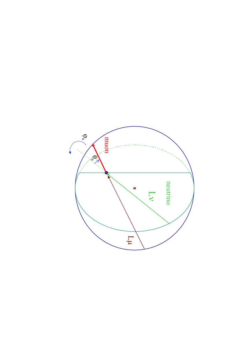
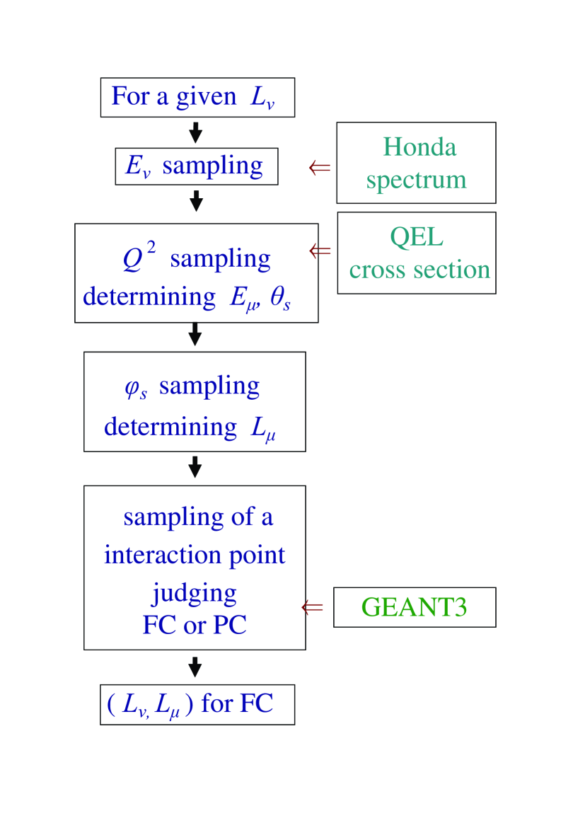
Figure 1: Schematic view of relations among $L_{\nu}$, $L_{\mu}$, $\theta_{s}$ and $\phi_{s}$ .

Figure 2: The procedure for our numerical experiment for obtaining $L_{\mu}$ from a given $L_{\nu}$.

In section 2 we give the procedure how to obtain $L_{\mu}$ from a neutrino event with given $L_{\nu}$ in stochastic manner. In section 3 we give the correlations between $L_{\nu}$ and $L_{\mu}$, taking into account of the effect of the backscattering as well as the effect of the azimuthal angle on the QEL in stochastic manner. As the result of it, we show that $L_{\nu}\approx L_{\mu}$, the SK assumption on the direction, does not hold even if statistically in both the absence and the presence of neutrino oscillation (Figure 3 and Figure 4). Also, we treat the correlation between $E_{\nu}$ and $E_{\mu}$, in stochastic manner. We show that the approximation of $E_{\nu}$ with $E_{\mu}$ by the Super-Kamiokande Collaboration does not make so serious error compared with the case of $L_{\nu}$ by $L_{\mu}$, although their treatment is theoretically unsuitable (Figure 5).

In section 4, we examine $L_{\nu}/E_{\nu}$ distribution and show the existence of the maximum oscillation under the neutrino oscillation parameters obtained by the Super-Kamiokande Collaboration, as it must be. This fact denotes that our numerical computer experiment is done in correct manner.

2 Generation of the Neutrino Events Occurring inside the Detector

In our numerical computer experiment, we obtain the Fully Contained Events resulting from QEL in the virtual SK detector, the details of which are described in Appendix A. For the neutrino event with a definite neutrino energy thus generated, we simulate its interaction point inside the detector and the emitted energy of the muon concerned which gives its scattering angle uniquely. The determination of the neutrino energy, the emitted energy of the muon and its scattering angle are described in the preceding paper ([4] see, the Appendices A,B and C in the preceding paper). The muon thus generated is pursued in the stochastic manner by using GEANT 3 and finally we judge whether the muon concerned stops inside the detector (the Fully Contained Event) or passes through the detector (the Partially Contained Event). For Fully Contained Events thus obtained, we know the directions of the incident neutrinos, the generation points and termination points of the events inside the detector, the emitted muon energies, their scattering angles and their azimuthal angles in QEL which lead finally their zenith angles, $L_{\nu}$ and $L_{\mu}$ .

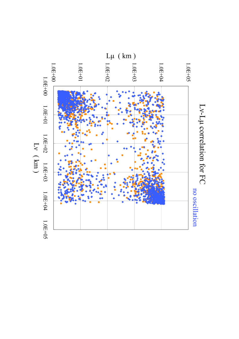
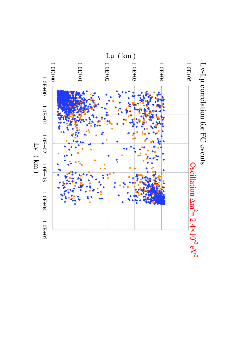
Figure 3: Correlation diagram for $L_{\nu}$ and $L_{\mu}$ without oscillation for for 1489.2 live days. The blue points and orange points denote neutrino events and ani-neutrino events, respectively.

Figure 4: Correlation diagram for $L_{\nu}$ and $L_{\mu}$ with the oscillation for 1489.2 live days. The blue points and orange points denote neutrino events and ani-neutrino events, respectively.

In Figure 2, we give the procedure for our numerical computer experiment. In our numerical computer experiment, we obtain $L_{\nu}$, $L_{\mu}$, $E_{\nu}$ and $E_{\mu}$. Therefore, we could choose four combinations among them, namely $L_{\nu}/E_{\nu}$, $L_{\mu}/E_{\mu}$, $L_{\mu}/E_{\nu}$ and $L_{\nu}/E_{\mu}$ for examination of maximum oscillations due to the neutrino oscillation. However, only the combination of $L_{\mu}/E_{\mu}$ out of these four combinations could be physically measurable. In the present paper(I) and a subsequent paper(II), we examine the relation between each combination and the oscillatory signature which is directly connected with the maximum oscillation in the presence of the neutrino oscillation. Our numerical computer experiments are being carried out for two different live days; namely, one is 1489.2 live days which is equal to the actual live days by Super-Kamiokande Experiment[6] and the other is 14892 days, ten times as much as the Super-Kamiokande Experiment actual live days.

3 Correlations between $L_{\nu}$ and $L_{\mu}$, and between $E_{\nu}$ and $E_{\mu}$

3.1 The correlation between $L_{\nu}$ and $L_{\mu}$

Super-Kamiokande Collaboration adopt the approximation of $L_{\nu}\approx L_{\mu}$ in their $L/E$ analysis [5]. As described in the preceding paper[4], the relation between direction cosine of the incident neutrino, $(\ell_{\nu(\bar{\nu})},m_{\nu(\bar{\nu})},n_{\nu(\bar{\nu})})$, and that of the corresponding emitted lepton, $(\ell_{\rm r},m_{\rm r},n_{\rm r})$, for a given scattering angle, $\theta_{\rm s}$, and its azimuthal angle, $\phi$, resulting from QEL is given as

$$\left(\begin{array}[]{c}\ell_{\rm{}_{\mu}}\\ m_{\rm{}_{\mu}}\\ n_{\rm{}_{\mu}}\end{array}\right)=\left(\begin{array}[]{ccc}\displaystyle\frac{\ell n}{\sqrt{\ell^{2}+m^{2}}}&-\displaystyle\frac{m}{\sqrt{\ell^{2}+m^{2}}}&\ell_{\nu(\bar{\nu})}\\ \displaystyle\frac{mn}{\sqrt{\ell^{2}+m^{2}}}&\displaystyle\frac{\ell}{\sqrt{\ell^{2}+m^{2}}}&m_{\nu(\bar{\nu})}\\ -\sqrt{\ell^{2}+m^{2}}&0&n_{\nu(\bar{\nu})}\end{array}\right)\left(\begin{array}[]{c}{\rm sin}\theta_{\rm s}{\rm cos}\phi\\ {\rm sin}\theta_{\rm s}{\rm sin}\phi\\ {\rm cos}\theta_{\rm s},\end{array}\right)$$ (2)

where $n_{\nu(\bar{\nu})}={\rm cos}\theta_{\nu(\bar{\nu})}$, and $n_{\rm{}_{\mu}}={\rm cos}\theta_{\mu}$. Here, $\theta_{\mu}$ is the zenith angle of the emitted muon.

$L_{\nu}$ and $L_{\mu}$ are functions of the direction cosine of the incident neutrino, $cos\theta_{\nu}$, and that of emitted muon, $cos\theta_{\mu}$, respectively and they are given as,

$$L_{\nu}=R_{g}\times(r_{SK}cos\theta_{\nu}+\sqrt{r_{SK}^{2}cos^{2}\theta_{\nu}+1-r_{SK}^{2}})\,\,\,\,(3-1)$$

$$L_{\mu}=R_{g}\times(r_{SK}cos\theta_{\mu}+\sqrt{r_{SK}^{2}cos^{2}\theta_{\mu}+1-r_{SK}^{2}})\,\,\,\,(3-2)$$

where $R_{g}$ is the radius of the Earth and $r_{SK}=1-D_{SK}/R_{g}$, with the depth, $D_{SK}$, of the Super-Kamiokande Experiment detector from the surface of the Earth. It should be noticed that the $L_{\nu}$ and $L_{\mu}$ are regulated by both the energy spectrum of the incident neutrino and the production spectrum of the muon and, consequently, their mutual relation is influenced by either the absence of the oscillation or the presence of the oscillation which depend on the combination of the oscillation parameters.

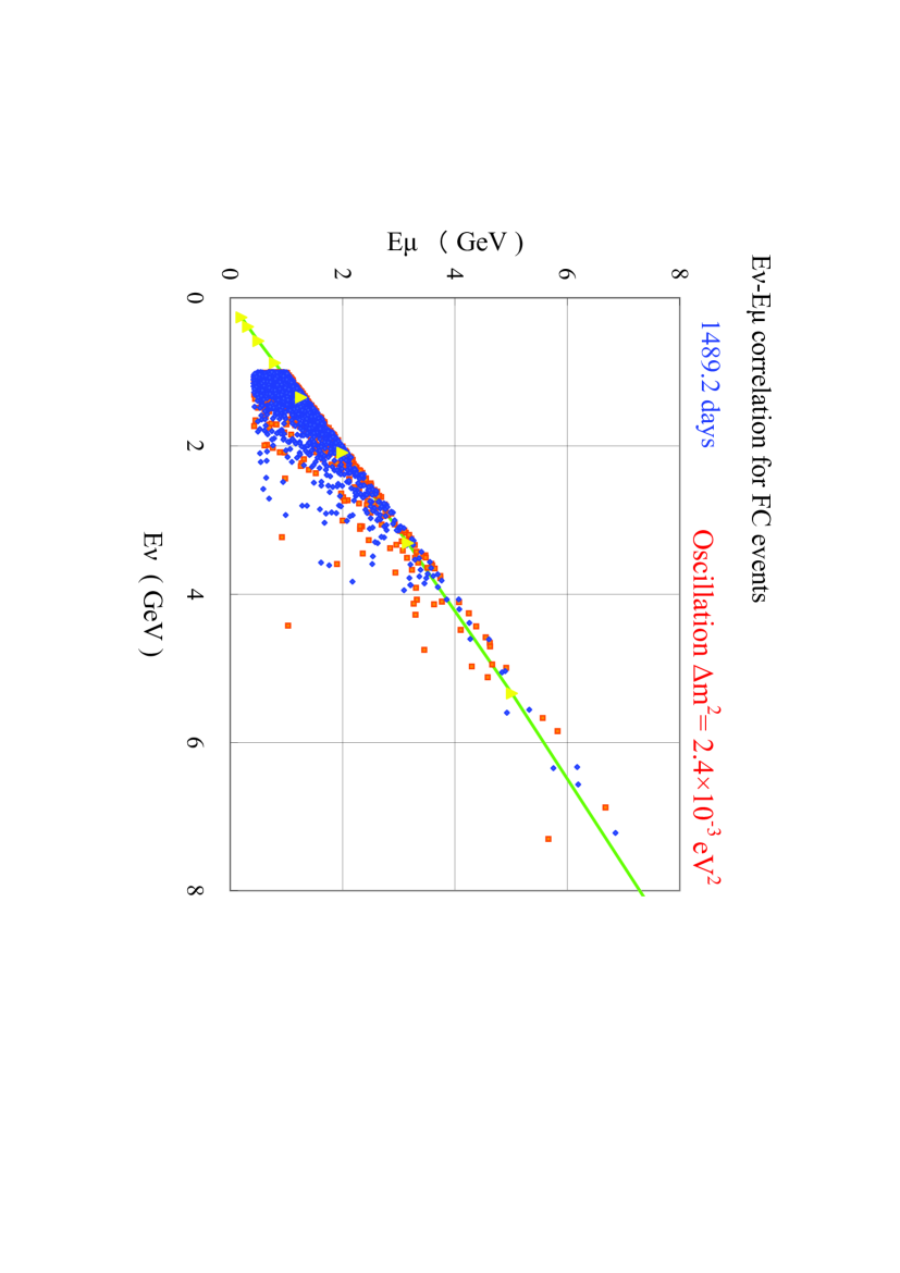
Figure 5: The correlation diagram between $E_{\nu}$ and $E_{\mu}$ for the oscillation. The continous line denotes the polynomial expression by the Super-Kamiokande Collabolation.

In Figure 3, we give the correlation diagram between $L_{\nu}$ and $L_{\mu}$ among Fully Contained Events for the 1489.2 live days in the absence of neutrino oscillation which corresponds to the actual Super-Kamiokande Experiment[6]. The aggregate of the (anti-) neutrino events which correspond to a definite combination of $L_{\nu}$ and $L_{\mu}$ are essentially classified into four groups in the following:

The group A is defined as the aggregate for neutrino events in which both $L_{\nu}$ and $L_{\mu}$ are rather smaller. It denotes that the downward neutrinos produce the downward muons. In this case, the energies of the produced muons are near the energies of the incident neutrinos due to smaller scattering angles.

The group B is defined as the aggregate for neutrino events in which both $L_{\nu}$ and $L_{\mu}$ are rather larger. It denotes that the upward neutrinos produce upward muons. In this case, the energy relation between the incident neutrinos and the produced muons is essentially the same as in the group A, because the flux of the upward neutrino events is symmetrical to that of the downward neutrino events in the absence of the neutrino oscillation.

The group C is defined as the aggregate for neutrino events in which $L_{\nu}$ are rather smaller and $L_{\mu}$ are rather larger. It denotes that the downward neutrinos produce the upward muons, namely by the possible effect reusulting from both backscattering and azimuthal angle in QEL, which is considered in the preceding paper [4]. In this case, the energies of the produced muon are rather smaller than those of the energies of the incident neutrinos due to larger scattering angles.

The group D is defined as the aggregate for the neutrino events in which $L_{\nu}$ are rather larger and $L_{\mu}$ are rather smaller. It denotes that the upward the neutrinos produce the downward muons The energy relation between the incident neutrinos and the produced muon is essentially the same as in the group C in the absence of the neutrino oscillation.

It is clear from the Figure 3 that there exist the symmetries between Group A and Group B, and also between Group C and Group D, which reflect the symmetry between the upward neutrino flux and the downward neutrino one for null oscillation.

In Figure 4, we give the correlation between $L_{\nu}$ and $L_{\mu}$ under their neutrino oscillation parameters, say, $\Delta m^{2}=2.4\times 10^{-3}\rm{eV^{2}}$ and $sin^{2}2\theta=1.0$ [6]. In the presence of the neutrino oscillation, the property of the symmetry which holds in the absence of the neutrino oscillation (see [group A and group B] and/or [group C and group D] in Figure 3) is lost due to the different incident neutrino fluxes in the upward direction and downward one. If we compare group A with group B, the event number in the group B (upward $\nu$ $\rightarrow$ upward $\mu$) is smaller than that in the group A (downward $\nu$ $\rightarrow$ downward $\mu$), which comes from smaller flux of the upward neutrinos. The similar relation between the group C (downward $\nu$ $\rightarrow$ upward $\mu$ ) and the group D (upward $\nu$ $\rightarrow$ downward $\mu$) is held in Figure 4.

Summarizing the characteristics among the groups A to D in the Figures 3 and 4, we could conclude that [group A and group B] and [group C and group D] are in symmetrical situations in the absence of the neutrino oscillation, while such the symmetrical situation is lost in the presence of the neutrino oscillation. Also, it is clear from the Figures 3 and 4 that $L_{\nu}\approx L_{\mu}$, the SK assumption on the direction does not hold both in the absence of the neutrino oscillation and in the presence of the neutrino oscillation even if statistically.

Here, it should be noticed that the approximation of $L_{\nu}\approx L_{\mu}$ could not hold completely in the region C and region D. The event number in the group C and group D could not be neglected among the total event number concerned. In these regions, neutrino events consist of those with backscattering and/or neutrino events in which the neutrino directions are horizontally downward (upward) but their produced muon turn to be upward (downward) resulting from the effect of azimuthal angles in QEL, respectively.

3.2 The correlation between $E_{\nu}$ and $E_{\mu}$

Super-Kamiokande Collaboration estimate $E_{\nu}$ from $E_{\mu}$, the visible energy of the muon, from their Monte Carlo simulation, by the following equation[2](p.135) :

$$E_{\nu,SK}=E_{\mu}\times(a+b\times x+c\times x^{2}+d\times x^{3}),\,\,\,(4)$$

where $x=log_{10}(E_{\mu})$.

The idea that $E_{\nu}$ could be approximated as the polynomial means that there is unique relation between $E_{\nu}$ and $E_{\mu}$. However, in the light of stochastic characters inherent in the incident neutrino energy spectrum and the production spectrum of the muon, such the treatment is not suitable theoretically, which may kill real correlation effect between the incident neutrino energy and the emitted muon energy. In Figure 5, we give the correlation between $E_{\nu}$ and $E_{\mu}$ together with that obtained from the polynomial expression by the Super-Kamiokande Collaboration under the their neutrino oscillation parameters. It is clear from the figure that the part of the lower energy incident neutrino deviates largely from the approximated formula, which reflects explicitly the stochastic character of the QEL. We could give the similar relation for null oscillation, the shape of which may be different from that with the oscillation due to the difference in the incident neutrino energy spectrum.

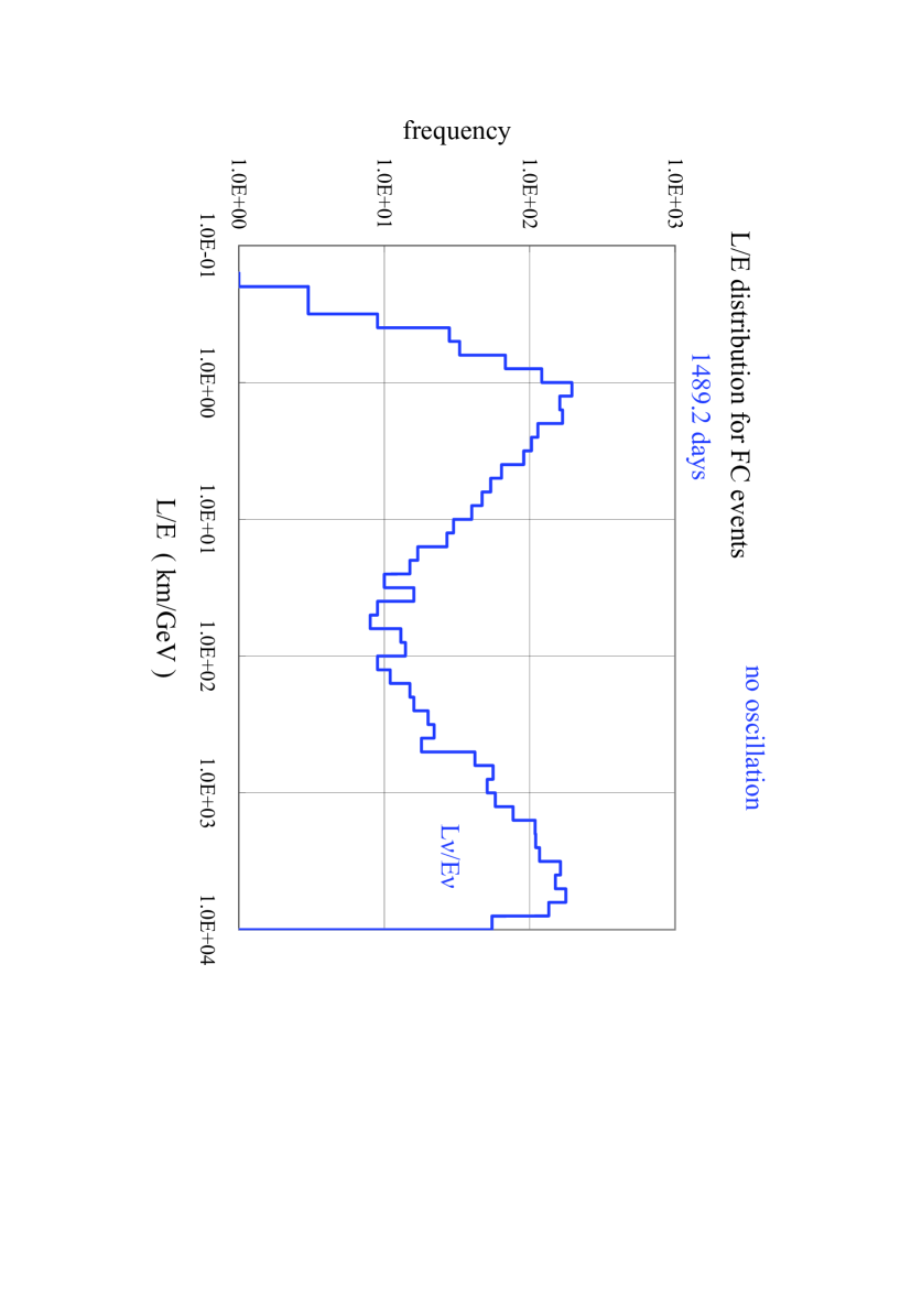
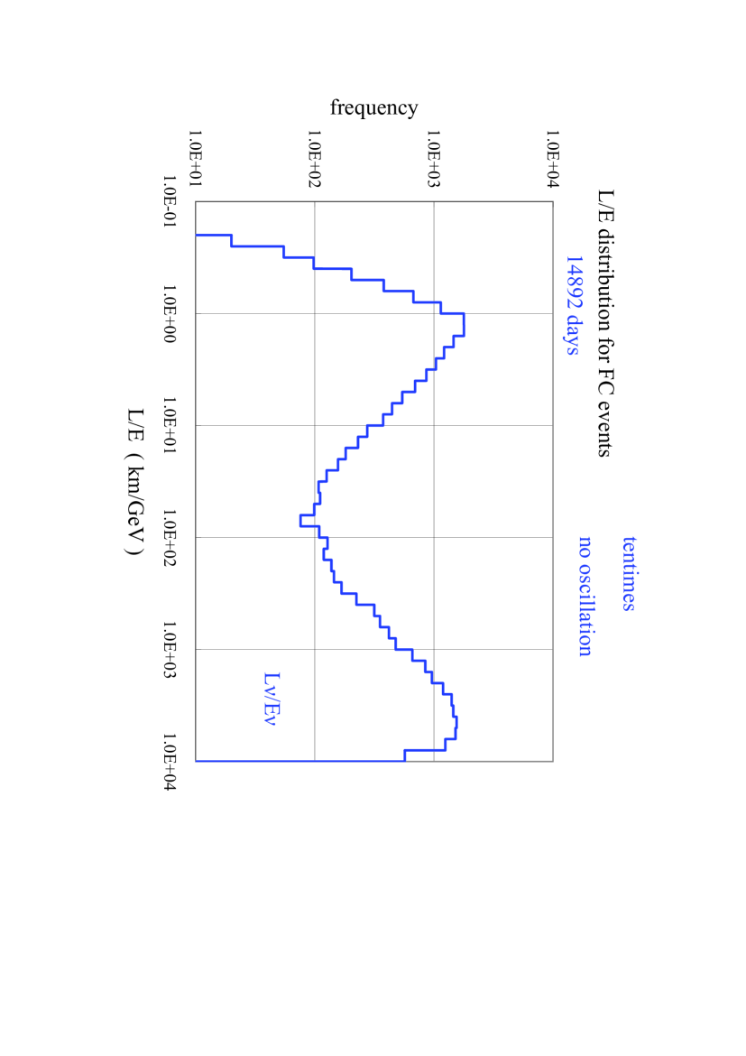
Figure 6: $L_{\nu}/E_{\nu}$ distribution without oscillation for 1489.2 live days.

Figure 7: $L_{\nu}/E_{\nu}$ distribution without oscillation for 14892 live days.

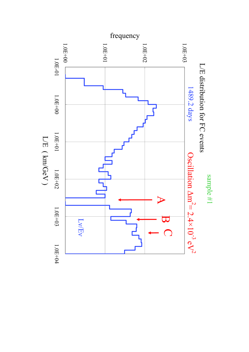
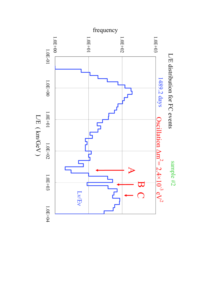
Figure 8: $L_{\nu}/E_{\nu}$ distribution with the oscillation for 1489.2 live days, sample 1.

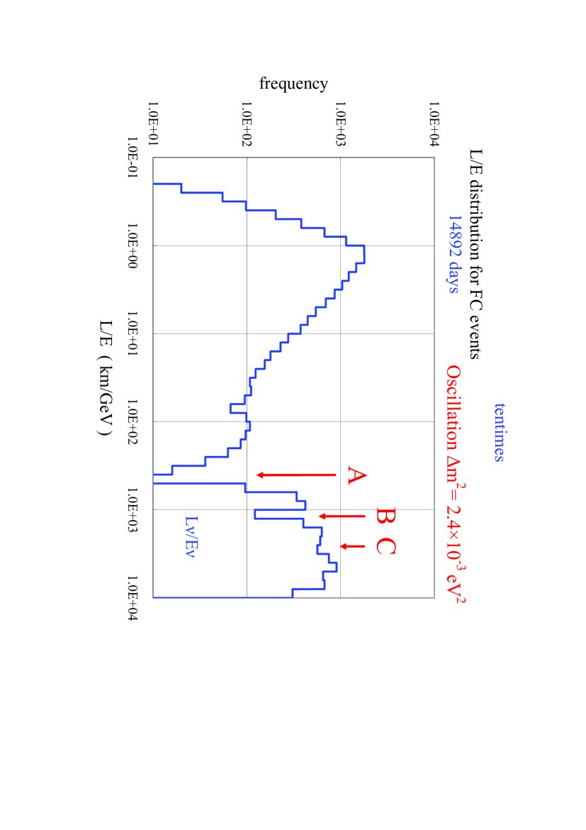
Figure 9: $L_{\nu}/E_{\nu}$ distribution with oscillation for 1489.2 live days, sample 2.

Figure 10: $L_{\nu}/E_{\nu}$ distribution with oscillation for 14892 live days.

4 $L_{\nu}/E_{\nu}$ Distributions in Our Numerical Experiment

4.1 For null oscillation

In Figures 6 and 7, we give $L_{\nu}/E_{\nu}$ distribution without oscillation for 1489.2 live days (SK live days[6]) and 14892 live days, respectively. Both distributions show the sinusoidal-like character for $L_{\nu}/E_{\nu}$ distribution, namely, the appearance of the top and the dip, appear even for null oscillation. The uneven histograms in Figure 6, comparing with those in Figure 7, show that the statistics of the Figure 6 is not enough compared with that of the Figure 7. Roughly speaking, smaller $L_{\nu}/E_{\nu}$ correspond to the contribution from downward neutrinos, larger one correspond to that from upward neutrino and $L_{\nu}/E_{\nu}$ near the dip correspond to the horizontal neutrinos, although the real situation is more complicated, because the backscattering effect as well as the azimuthal angle effect could not be neglected. From Figure 7, we understand that the dip around 70 km/GeV denotes the contribution from the horizontal direction.

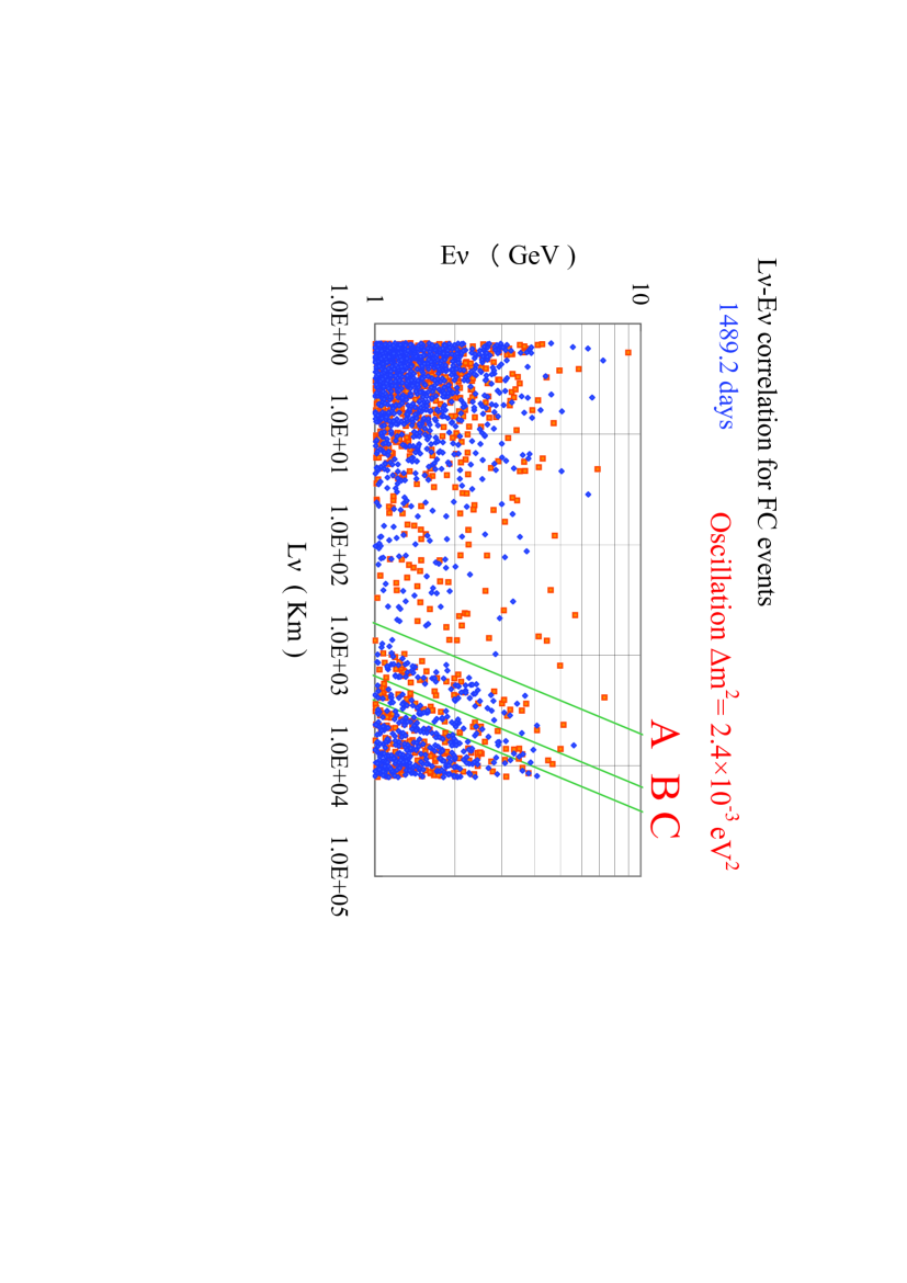
Figure 11: The correlation diagram between $L_{\nu}$ and $E_{\nu}$ with oscillation for 1489.2 live days.

Figure 12: The correlation diagram between $L_{\nu}$ and $E_{\nu}$ with oscillation for 14892 live days.

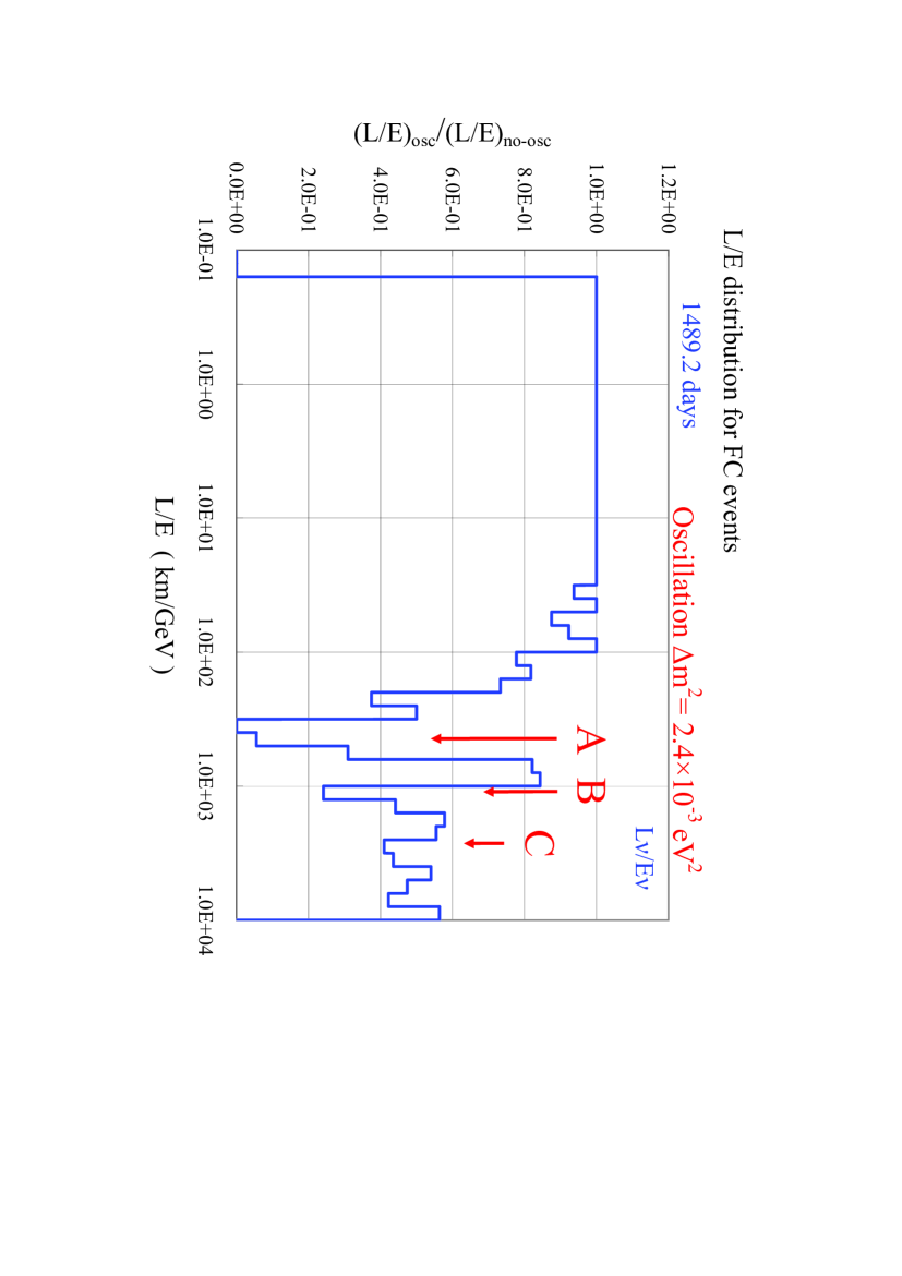
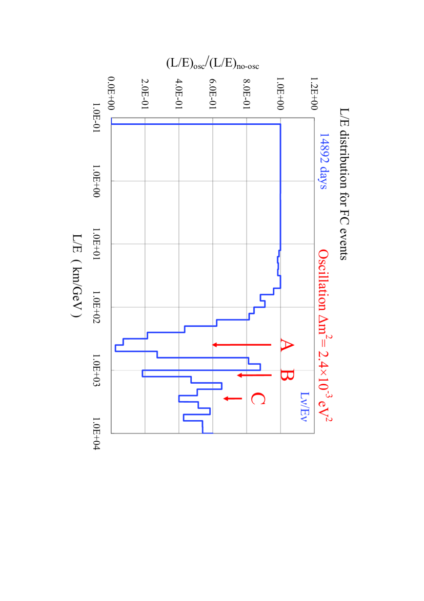
Figure 13: The ratio of $(L_{\nu}/E_{\nu})_{osc}/(L_{\nu}/E_{\nu})_{null}$ for 1489.2 live days.

Figure 14: The ratio of $(L_{\nu}/E_{\nu})_{osc}/(L_{\nu}/E_{\nu})_{null}$ for 14892 live days.

4.2 For the oscillation (SK oscillation parameters)

Super-Kamiokande Collaboration analyze experimental data consisting of Fully Contained Events and Partially Contained Events (single ring mu-like events and multi-ring mu-like events) on the $L/E$ distribution, expecting to find their oscillatory signature, say, the presence of maximum osccillations, and they claim that they find a dip near 500 km/GeV which is consistent with their neutrino oscillation parameters $\Delta m^{2}=2.4\times 10^{-3}\rm{eV^{2}}$ and $sin^{2}2\theta=1.0$[6].

The survival probability of a given flavor, such as $\nu_{\mu}$, is given by

$$P(\nu_{\mu}\rightarrow\nu_{\mu})=1-sin^{2}2\theta sin^{2}(1.27\Delta m^{2}L_{\nu}/E_{\nu}).\,\,\,(5)$$

Then, for maximum oscillation under SK neutrino oscillation parameters, we have

$$1.27\Delta m^{2}L_{\nu}/E_{\nu}=(2n+1)\times\frac{\pi}{2},\,\,\,\,\,\,(6)$$

where $\Delta m^{2}=2.4\times 10^{-3}\rm{eV^{2}}$. From the eqation, we have the following values of $L_{\nu}/E_{\nu}$ for maximum oscillations.

$$L_{\nu}/E_{\nu}=515{\rm km/GeV}\,\,\,for\,\,n=1\,\,\,(7-1)$$

$$1540{\rm km/GeV}\,\,\,for\,\,n=2\,\,\,(7-2)$$

$$2575{\rm km/GeV}\,\,\,for\,\,n=3\,\,\,(7-3)$$

In Figures 8 and 9, we give the $L_{\nu}/E_{\nu}$ distributions with the oscillation for one unit of 1489.2 live days and the another unit of 1489.2 live days, respectively. In Figure 8, we could observe the first maximum oscillation (Eq.7-1, arrow A) and the second(Eq.7-2, arrow B) clearly, and the third (Eq.7-3, arrow C) faintly, which means not enough statistics for the confirming the existence of the third maximum oscillation. In Figure 9, we could observe similar situation for another 1489.2 live days as observed in Figure 8. In Figure 10, we give the $L_{\nu}/E_{\nu}$ distribution with the oscillation for 14892 live days being ten times as much as those of Figures 8 and 9. In Figure 10, we could observe a more narrower dip which corresponds to the first maximum oscillation due to ten times statistics as much as those of Figures 8 and 9. Also, we could observe the second maximum oscillation clearly, too. However, it is a little bit difficult to observe the third maximum oscillation for even larger statistics.

In Figure 11, we give the correlation between $L_{\nu}$ and $E_{\nu}$ which is obtained from the same data as in Figure 8. The linearly strip patterns in which there are absent from the combinations of $L_{\nu}$ and $E_{\nu}$, correspond to the first, the second and third maximum in the $L_{\nu}/E_{\nu}$ distribution. In Figure 12, we give the same correlation for 14892 days being ten times larger than the Super-Kamiokande Experiment actual live days. Compared Figure 12 with Figure 11, the larger statistics show more clear strip pattern which correspond to more clear existence of the maximum oscillation as in the Figure 10. Lines A, B and C in Figures 11 and 12 correspond to Eqs.(7-1),(7-2) and (7-3) respectively. Surely, we observe dips characterized by these lines where we have no events. Namely, these figures show the presence of the maximum oscillation obtained from Eq.(6).

From the point of view of the numerical computer experiment, the survival probability of a given flavor is give as the ratio of $(L_{\nu}/E_{\nu})_{osc}/(L_{\nu}/E_{\nu})_{null}$. In Figures 13 and Figure 14, these ratios are given for 1489.2 live days and 14892 live days being ten times as much as 1489.2 live days, respectively. These ratios indicate the presence of the maximum oscillations shown as arrows A, B and C. Comparing the ratio of 1489.2 live days with that of 14892 live days in the light of their smoothness, it seems that statistics with 1489.2 live days are not so beautiful compared to statistics with 14892 live days.

Now, it is concluded from Figures 8 to 14 that our numerical computer experiments are carried out in a correct way, which shows really the sinusoidal flavor transition probability of neutrino oscillation under the neutrino oscillation parameters by the Super-Kamiokande Collaboration, if they really exist. However, at the same time, it should be noticed that such neutrino oscillatory signature could not be observed really at all even if it really exists, because both the physical quantities, $L_{\nu}$ and $E_{\nu}$, are not physical observables.

5 Summary

In our numerical computer experiment, we have found the existence of the maximum oscillation, 515km/GeV, 1540km/GeV and 2575km/GeV, under the neutrino oscillation parameter ($\Delta m^{2}=2.4\times 10^{-3}\rm{eV^{2}}$ and $sin^{2}2\theta=1.0$ ), successfully, as they should be. It denotes that our numerical computer experiment have been done in correct way. Both $L_{\nu}$ and $E_{\nu}$ could not be measurable, because neutrinos are neutral. Consequently, even if the neutrino oscillation exist really, we could not detect neutrino oscillation from $L_{\nu}/E_{\nu}$ analysis. In the subsequent paper, we examine whether the maximum oscillation resulting from the neutrino oscillation through the analysis of other possible combinations of L/E, such as $L_{\nu}/E_{\mu}$, $L_{\mu}/E_{\nu}$ and $L_{\mu}/E_{\mu}$, can be detected or not.

Appendix A Appendix: Detection of the Neutrino Events in the SK Detector and Their Interaction Points

The plane ABCD is always directed vertically to the direction of the incident neutrino with a given zenith angle, which is shown in Fig. 15. The rectangular ABCDEFGH encloses the detector of the Super-Kamiokande Experiment whose radius and height are denoted by R and H, respectively. The width and the height of the plane ABCD for a given zenith angle, ${\theta_{\nu(\bar{\nu})}}$, are given as, R and R$\cos\theta_{\nu(\bar{\nu})}$ + H$\sin{\theta}_{\nu}$, respectively, which are shown in Fig. A1-(c).

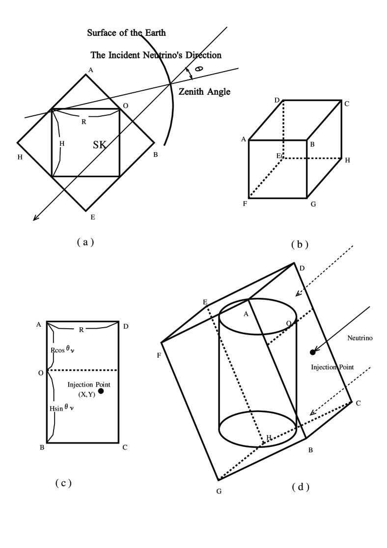
Figure 15: Sampling procedure for neutrino evens injected into the detector

Now, let us estimate the ratio of the number of the neutrino events inside the detector of the Super-Kamiokande Experiment to that in the rectangular ABCDEFGH. As the number of the neutrino events inside some material is proportional to the number of the nucleons in the material concerned. The number of the nucleons inside the SK detector $(\rho=1)$ is given as

$$N_{\rm sk}=\frac{\pi}{4}N_{\rm avoga}R^{2}H,$$ (A·1)

where $N_{\rm avoga}$ denotes the Avogadro number, and the number of the nucleons in the exterior of the detector inside ABCDEFGH is given as

$$N_{\rm extr}(\cos\theta_{\nu(\bar{\nu})})=\rho N_{\rm avoga}\biggl{[}\biggl{(}1-\frac{\pi}{4}\biggr{)}R^{2}H+R(H^{2}\!\!+\!\!R^{2})\sin{\theta}_{\nu(\bar{\nu})}\cos\theta_{\nu(\bar{\nu})}\biggr{]},$$ (A·2)

where $\rho$ is the density of the rock which surrounds the SK detector.

Then, the total number of the target in the rectangularABCDEFGH is given as

$$N_{\rm tot}(\cos\theta_{\nu(\bar{\nu})})=N_{\rm sk}+N_{\rm extr}(\cos\theta_{\nu(\bar{\nu})}).$$ (A·3)

Here, we take 2.65 as ${\rho}$ (standard rock).

Then, $R_{\rm theor}$, the ratio of the number of the neutrino events in the SK detector to that in the rectangular ABCDEFGH is given as

$$R_{\rm theor}(\cos\theta_{\nu(\bar{\nu})})=N_{\rm sk}/N_{\rm tot}(\cos\theta_{\nu(\bar{\nu})}).$$ (A·4)

We obtain $R_{\rm theor}$ for different values of $\cos{\theta_{\nu(\bar{\nu})}}$ given in the Table 1.
Here, we simulate neutrino events occured in the rectangular ABCDEFH, by using the atmospheric neutrino beam which falls down on the plane ABCD. Thus, $N_{\rm smaple}$, the sampling number of the (anti-)neutrino events inside the rectangular ABCDEFG for a given ${\cos\theta_{\nu(\bar{\nu})}}$ is given as

$$N_{\rm sample}(\cos\theta_{\nu(\bar{\nu})})=N_{\rm tot}(\cos\theta_{\nu(\bar{\nu})})\times$$

$$\int_{E_{\nu(\bar{\nu}),{\rm min}}}^{E_{\nu(\bar{\nu}),{\rm max}}}\sigma_{{}_{\ell(\bar{\ell})}}(E_{\nu(\bar{\nu})})N_{\rm int}(E_{\nu(\bar{\nu})},t,{\rm cos}\theta_{\nu(\bar{\nu})}){\rm d}E_{\nu(\bar{\nu})}$$

where $\sigma_{\ell(\bar{\ell})}(E_{\nu(\bar{\nu})})$ is the total cross section for (anti-)neutrino due to QEL, and $N_{\rm int}(E_{\nu(\bar{\nu})},t,{\rm cos}\theta_{\nu(\bar{\nu})}){\rm d}E_{\nu(\bar{\nu})}$ is the differential nutrino energy spectrum for the definite zenith angle, $\theta_{\nu(\bar{\nu})}$, in the plane ABCD. The injection points of the neutrinos in the plane ABCD are distributed over the plane randomly and uniformely and the injection points are determined from a pair of the uniform random numbers between (0,1). They penetrate into the rectangular ABCDEFGH from the injection point in the plane ABCD and some of them may penetrate into the SK detector or may not, which depend on their injection point.

In the neutrino events which penetrate into the SK detector, their geometrical total track length, $T_{\rm track}$, are devided into three parts

$$T_{\rm track}=T_{\rm b}+T_{\rm sk}+T_{\rm a},$$ (A·6)

where $T_{\rm b}$ denotes the track length from the plane ABCD to the entrance point of the SK detector, $T_{\rm sk}$ denotes the track length inside the SK detector, and $T_{\rm a}$ denotes the track length from the escaping point of the SK detector to the exit point of the rectangular ABCDEF, and thus $T_{\rm track}$ denotes the geometrical length of the neutrino concerned in the rectangular ABCDEFGH.

By the definition, the neutrinos concerned with $T_{\rm track}$ interact surely somewhere along the $T_{\rm track}$. Here, we are interested only in the interaction point which occurs along $T_{\rm sk}$. We could determine the interaction point in the $T_{\rm sk}$ in the following.

We define the following quantities for the purpose.

$$T_{\rm weight} = T_{\rm sk}+\rho(T_{\rm b}+T_{\rm a}),$$ (A·7)

$$\rho_{\rm av} = T_{\rm weight}/T_{\rm track},$$ (A·8)

$$\xi_{\rho} = \rho_{\rm av}/\rho,$$ (A·9)

$$\xi_{\rm sk} = T_{\rm sk}/T_{\rm weight}.$$ (A·10)

The flow chart for the choice of the neutrino events in the SK detector and the determination of the interaction points inside the SK detector is given in Fig. 16. Thus, we obtain neutrino events whose occurrence point is decided in the SK detector in the following.

Figure 16: Flow Chart for the determination of the interaction points of the neutrino events inside the detector

$$x_{f} = x_{0},$$ (A·11)

$$y_{f} = y_{0}+\xi T_{\rm sk}\sin{\theta}_{\nu(\bar{\nu})}$$ (A·12)

$$z_{f} = z_{0}+\xi T_{\rm sk}\cos\theta_{\nu(\bar{\nu})}.$$ (A·13)

If we carry out the Monte Carlo Simulation, following the flow chart in Fig. 16, then, we obtain $N_{\rm event}$, the number of the neutrino events generasted in the SK detector. The ratio of the selected events to the total trial is given as

$$R_{\rm monte}(\cos\theta_{\nu(\bar{\nu})})=N_{\rm event}(\cos\theta_{\nu(\bar{\nu})})/N_{\rm sample}(\cos\theta_{\nu(\bar{\nu})}).$$ (A·14)

Comparison between $R_{\rm theor}$ and $R_{\rm monte}$ in Table A1 shows that our Monte Carlo procedure is valid.

Table 1: Occurrence probabilities of the neutrino events inside the SK detector for different $\cos\theta_{\nu}$’s. Comparison between $R_{\rm theor}$ and $R_{\rm monte}$. The sampling numbers for the Monte Carlo Simulation are, 1000, 10000, 100000, respectively.

cos $\theta_{\nu}$	$R_{\rm{theor}}$	$R_{\rm{monte}}$
		Sampling Number
		1000	10000	100000
0.000	0.58002	0.576	0.5750	0.57979
0.100	0.41717	0.425	0.4185	0.41742
0.200	0.32792	0.353	0.3252	0.32657
0.300	0.27324	0.282	0.2731	0.27163
0.400	0.23778	0.223	0.2329	0.23582
0.500	0.21491	0.206	0.2063	0.21203
0.600	0.20117	0.197	0.1946	0.19882
0.700	0.19587	0.193	0.1925	0.19428
0.800	0.20117	0.198	0.2002	0.20001
0.900	0.22843	0.230	0.2248	0.22803
1.00	0.58002	0.557	0.5744	0.57936

References

References

- [1] Kajita, T. and Totsuka, Y. Rev. Mod. Phys., 73 (2001)85. See p.101.
- [2] Ishitsuka, M., PhD thesis, University of Tokyo (2004). See p. 138.
- [3] Jung, CK., Kajita, T., Mann TC. and McGrew, C., Anual. Rev. Nucl. Sci. vol.15 (2005) 431. See p.453
- [4] Konishi,E.,Minorikawa,Y.,Galkin,V.I.,Ishiwata,M., Nakamura,I.,Kato,M. and Misaki,A arXiv:hep-ex/0808.0664v2
- [5] Ashie,Y et al., Phys.Rev.Lett.93(2004)101801-1
- [6] Ashie,Y et al., Phys.Rev.D171(2005)112005