Magnetization of a half-quantum vortex in a spinor Bose-Einstein condensate

Abstract

Magnetization dynamics of a half-quantum vortex in a spin-1 Bose-Einstein condensate with a ferromagnetic interaction are investigated by mean-field and Bogoliubov analyses. The transverse magnetization is shown to break the axisymmetry and form threefold domains. This phenomenon originates from the topological structure of the half-quantum vortex and spin conservation.

I Introduction

The spin degrees of freedom in an atomic Bose-Einstein condensate (BEC) allow for a variety of topological defects. Mermin-Ho Mermin and Anderson-Toulouse Anderson vortices have been produced by the MIT group Leanhardt03 using the topological phase-imprinting method Leanhardt02 . Recently, the Berkeley group observed spontaneous formation of polar-core vortices in magnetization of a spin-1 ${}^{87}{\rm Rb}$ BEC Sadler . In addition, several theoretical predictions have been made of various topological defects in spinor BECs, such as fractional vortices Volovik ; Leonhardt ; Zhou , skyrmions Khawaja , and knot structures Kawaguchi .

Topological-defect structures in spinor BECs are closely related to the symmetry groups of spin states Ho . For example, the symmetry group of the polar state ($m=0$, where $m$ denotes the magnetic sublevel of the spin) in a spin-1 BEC is ${\rm U(1)}\times S^{2}/{\rm Z}_{2}$, and distinct configurations of the polar state can be specified by elements of this group. This symmetry group allows the topological structure of the half-quantum vortex Volovik ; Leonhardt ; Zhou . On the other hand, the symmetry group of the ferromagnetic state ($|m|=1$) in a spin-1 BEC is SO(3).

Let us consider a half-quantum vortex prepared in an antiferromagnetic BEC. We then consider a magnetic phase transition occurring from the antiferromagnetic to ferromagnetic phases. Since the symmetry group of the spin state changes from ${\rm U(1)}\times S^{2}/{\rm Z}_{2}$ to SO(3) and the half-quantum vortex structure cannot exist for the latter symmetry group, the ensuing magnetization dynamics are expected to break the symmetry and create nontrivial states. Such a change of spin texture associated with a change of the spin state symmetry group is the subject of the present paper.

In the present paper, we study the magnetization dynamics of the half-quantum vortex state produced in a spin-1 ferromagnetic BEC. The initial state can be prepared by, e.g., the phase-imprinting method using Laguerre-Gaussian beams Andersen . We show that the half-quantum vortex develops into threefold magnetic domains through dynamical instability. This contrasts with the magnetization of a uniform polar state, in which a polar-core vortex or twofold domain structure is formed SaitoL . We study the dynamical instability using the Bogoliubov analysis, numerically in a 2D system and analytically in a 1D ring. The threefold domain formation can also be understood from the topological structure of a half-quantum vortex and spin conservation, and its geometrical interpretation is provided.

This paper is organized as follows. Section II introduces the formulation of the problem and defines the notation used. Section III shows the magnetization dynamics of the half-quantum vortex and demonstrates threefold domain formation. Section IV details the Bogoliubov analysis to study the dynamical instability. Section V is devoted to the geometrical interpretation of the threefold domain formation. Section VI gives the conclusions to the study.

II Formulation of the problem

We consider a BEC of spin-1 atoms with mass $M$ confined in an axisymmetric harmonic potential $V(\bm{r})=M[\omega_{\perp}^{2}(x^{2}+y^{2})+\omega_{z}^{2}z^{2}]/2$ that is independent of the magnetic sublevels $m$ of the spin. In the mean-field approximation, the condensate can be described by the macroscopic wave functions $\psi_{m}(\bm{r})$ with $m=-1,0,1$ satisfying

$$\int d\bm{r}\sum_{m=-1}^{1}|\psi_{m}|^{2}\equiv\int d\bm{r}\rho=N,$$ (1)

where $N$ is the number of atoms. The magnetization density is given by

$$\bm{F}=\sum_{m,m^{\prime}}\psi_{m}^{*}\bm{f}_{mm^{\prime}}\psi_{m^{\prime}},$$ (2)

where $\bm{f}$ is the vector of the spin-1 matrices. The macroscopic wave functions at zero temperature obey the three-component Gross-Pitaevskii (GP) equations,

$$i\hbar\frac{\partial\psi_{0}}{\partial t} = \left(-\frac{\hbar^{2}}{2M}\nabla^{2}+V+c_{0}\rho\right)\psi_{0}$$ (3a)

$$+\frac{c_{1}}{\sqrt{2}}\left(F_{+}\psi_{1}+F_{-}\psi_{-1}\right),$$

$$i\hbar\frac{\partial{\psi_{\pm 1}}}{\partial t} = \left(-\frac{\hbar^{2}}{2M}{\nabla}^{2}+V+c_{0}\rho\right)\psi_{\pm 1}$$ (3b)

$$+c_{1}\left(\frac{1}{\sqrt{2}}F_{\mp}\psi_{0}\pm F_{z}\psi_{\pm 1}\right),$$

where $F_{\pm}=F_{x}\pm iF_{y}$. The interaction coefficients in Eq. (3) are defined as

$$c_{0}=\frac{4\pi\hbar^{2}}{M}\frac{a_{0}+2a_{2}}{3},\qquad c_{1}=\frac{4\pi\hbar^{2}}{M}\frac{a_{2}-a_{0}}{3},$$ (4)

with $a_{0}$ and $a_{2}$ being the $s$-wave scattering lengths for colliding channels with total spins 0 and 2. For $c_{1}<0$, the ferromagnetic state is energetically favorable, while for $c_{1}>0$ the polar or antiferromagnetic state is favorable. In the present paper, we restrict ourselves to spin-1 ${}^{87}{\rm Rb}$ atoms, which have a positive $c_{0}$ and a negative $c_{1}$ Schmal .

We assume that $\hbar\omega_{z}$ is much larger than other characteristic energies and the condensate has a tight pancake shape. The condensate wave function is therefore frozen in the ground state of the harmonic potential in the $z$ direction and the system is effectively 2D. Integrating the GP energy functional with respect to $z$, we find that the 2D wave function $\psi_{m}^{\rm 2D}$ follows the GP equation having the same form as Eq. (3), where the interaction coefficients $c_{0}$ and $c_{1}$ are multiplied by $[m\omega_{z}/(2\pi\hbar)]^{1/2}$. We define a normalized wave function,

$$\tilde{\psi}_{m}=\frac{1}{\sqrt{N}}\frac{\hbar}{m\omega_{\perp}}\psi_{m}^{\rm 2D},$$ (5)

and normalized interaction coefficients,

$$\tilde{c}_{j}=\frac{N}{\hbar\omega_{\perp}}\sqrt{\frac{m\omega_{z}}{2\pi\hbar}}\frac{m\omega_{\perp}}{\hbar}c_{j}$$ (6)

with $j=0$ and $1$. For example, using the scattering lengths of a spin-1 ${}^{87}{\rm Rb}$ atom $a_{0}=101.8a_{\rm B}$ and $a_{2}=100.4a_{\rm B}$ Kempen , where $a_{\rm B}$ is the Bohr radius, and trap frequencies $\omega_{\perp}=2\pi\times 200$ Hz and $\omega_{z}=2\pi\times 4$ kHz, the interaction coefficients become

$$\tilde{c}_{0}\simeq 0.16N,\;\;\;\;\tilde{c}_{1}\simeq-\tilde{c}_{0}/216.$$ (7)

We consider a half-quantum vortex state given by Leonhardt

$$\left(\begin{array}[]{c}\psi_{1}^{\rm hqv}\\ \psi_{0}^{\rm hqv}\\ \psi_{-1}^{\rm hqv}\end{array}\right)=\left(\begin{array}[]{c}{f_{1}(r)}e^{\pm i\theta}\\ 0\\ {f_{-1}(r)}\end{array}\right),$$ (8)

where $r=(x^{2}+y^{2})^{1/2}$ and $\theta={\rm arg}(x+iy)$. The functions $f_{\pm 1}(r)$ are stationary solutions of Eq. (3) satisfying

$$\int_{0}^{\infty}2\pi r^{2}|f_{\pm 1}(r)|^{2}dr=\frac{N}{2}.$$ (9)

From this condition, the state (8) has an angular momentum of $N\hbar/2$. Without loss of generality, we restrict ourselves to the upper sign in Eq. (8) unless otherwise stated.

As several authors have discussed Volovik ; Leonhardt ; Zhou , the half-quantum vortex has an interesting topological structure. Equation (8) is invariant under the transformation $\exp(i\phi/2)\exp(if_{z}\phi/2)\exp(-\phi\partial_{\theta})$, where $\phi$ is an arbitrary angle and $f_{z}=m$ for $\psi_{m}$. This indicates that spatial rotation by an angle $\phi$ around the $z$ axis is accompanied by spin rotation by $-\phi/2$ with an additional phase factor $\exp(i\phi/2)$. Thus, for a rotation around the $z$ axis by $2\pi$, the spin rotates only by $-\pi$.

Thermodynamic stability of the half-quantum vortex is studied in Ref. Isoshima , while a half-quantum vortex ring is discussed in Ref. Ruo . Recently, it has been predicted that half-quantum vortices can be nucleated in rotating traps Ji ; Chiba and fluctuation-drive vortex fractionalization has been proposed in Ref. Song .

III Magnetization dynamics of a half-quantum vortex

In this section, we study the magnetization dynamics of the half-quantum vortex state (8) for a spin-1 ${}^{87}{\rm Rb}$ BEC.

The initial state is assumed to be the half-quantum vortex state (8) obtained by the imaginary-time propagation method. An experimental method to realize this initial state is discussed later. It follows from Eq. (3) that when $\psi_{0}$ is exactly zero as in Eq. (8), $\psi_{0}$ always vanishes in the mean-field evolution and no magnetization occurs even for a ferromagnetic interaction. We therefore add a small amount of initial noise to $\psi_{0}$, which triggers growth of the $m=0$ component. Physically, this initial noise corresponds to quantum and thermal fluctuations and experimental imperfections SaitoL ; SaitoA ; SaitoKZ . We set the noise as $\tilde{\psi}_{0}=r_{1}+ir_{2}$ on each mesh point, where $r_{1}$ and $r_{2}$ are random numbers with uniform distribution between $\pm 10^{-3}$. For the imaginary- and real-time propagations, we employ the Crank-Nicolson method with the size of each mesh being 0.05 $\sqrt{\hbar/(m\omega_{\perp})}$.

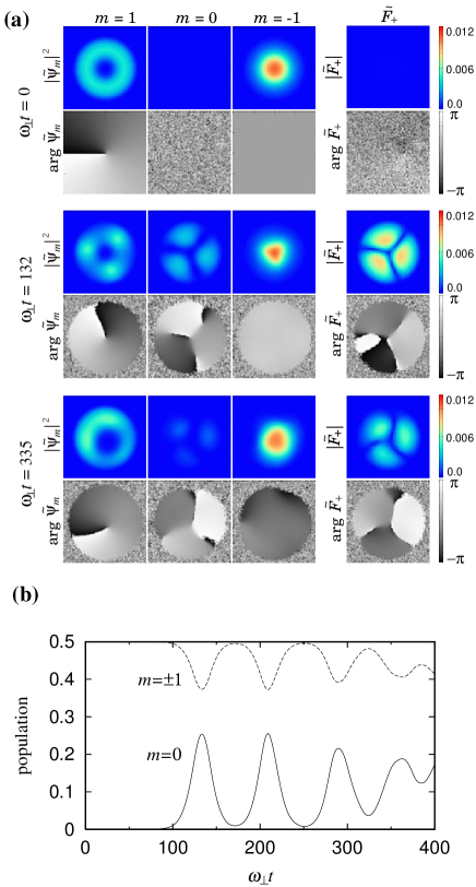
Figure 1: (color) (a) Time evolution of the normalized wave function $\tilde{\psi}_{m}$ and transverse magnetization $\tilde{F}_{+}=\tilde{F}_{x}+i\tilde{F}_{y}$, where $\tilde{F}_{x}$ and $\tilde{F}_{y}$ are defined by Eq. (2) with $\psi_{m}$ replaced by $\tilde{\psi}_{m}$. The size of each panel is $10\times 10$ in units of $\sqrt{\hbar/(m\omega_{\perp})}$. (b) Time evolution of the population in each component. The interaction coefficients are $\tilde{c}_{0}=3000$ and $\tilde{c}_{1}=-\tilde{c}_{0}/216$ (corresponding to spin-1 ${}^{87}{\rm Rb}$).

Figure 1 (a) shows the time evolution of the density and phase profiles of each spin component and that of the transverse magnetization. At $\omega_{\perp}t=0$, the transverse magnetization almost vanishes because of the initial state (8) with small noise added in the $m=0$ component. The $m=0$ component then grows in time and exhibits a threefold pattern, which leads to threefold magnetic domains as shown in Fig. 1 (a) ($\omega_{\perp}t=132$). This threefold domain formation is the main result of the present paper. We note that the magnetization in the three domains have different directions to cancel and conserve the total spin. Then, the population for each $m$ oscillates as shown in Fig. 1 (b) due to the excess energy, and the appearance and disappearance of the threefold domains are repeated. At $\omega_{\perp}t\simeq 300$, the instability in the dipole mode becomes significant and the system undergoes a dipole deformation as shown in Fig. 1 (a), which is followed by complicated dynamics. Throughout the dynamics, the total density profile is almost unchanged and remains in the Thomas-Fermi distribution. The threefold domains are generated for both signs in the initial state (8). We checked that no dynamics occur for an antiferromagnetic interaction ($c_{1}>0$).

We now discuss how to prepare the initial state in an experiment. First we create a non-rotating BEC in the $m=-1$ component, $\psi_{-1}^{\rm ini}$, and then Gaussian and Laguerre-Gaussian beams propagating in the same direction are applied. The frequencies of these beams are tuned to the Raman transition from the non-rotating $m=-1$ state to the $m=1$ state with a unit angular momentum Andersen . We thus obtain the half-quantum vortex state given by

$$\left(\begin{array}[]{c}\psi_{1}\\ \psi_{0}\\ \psi_{-1}\end{array}\right)=\left(\begin{array}[]{c}\psi_{-1}^{\rm ini}e^{i\theta}\sin(Are^{-Br^{2}})\\ 0\\ \psi_{-1}^{\rm ini}\cos(Are^{-Br^{2}})\end{array}\right),$$ (10)

where $A$ and $B$ are proportional to the intensity and width of the beams, respectively. For example, $A=0.196(m\omega_{\perp}/\hbar)^{1/2}$ and $B=0.002m\omega_{\perp}/\hbar$ give density profiles similar to the initial state in Fig. 1. We have confirmed that the dynamics from this initial state are qualitatively the same as those in Fig. 1. The pattern formation as shown in Fig. 1 (a) can be observed using the Stern-Gerlach separation and a nondestructive spin-sensitive measurement Higbie .

IV Bogoliubov analysis

IV.1 Numerical diagonalization

The dynamics shown in Fig. 1 suggest that the half-quantum vortex state has dynamical instabilities. In this section, we perform the Bogoliubov analysis.

We decompose the macroscopic wave functions $\psi_{m}$ into the stationary state $\psi_{m}^{\rm hqv}$ in Eq. (8) and small deviations $\delta\psi_{m}$ from this state as

$$\left(\begin{array}[]{c}\psi_{1}\\ \psi_{0}\\ \psi_{-1}\end{array}\right)=\left(\begin{array}[]{c}e^{-i\mu_{1}t/\hbar}(\psi_{1}^{\rm hqv}+\delta\psi_{1})\\ e^{-i(\mu_{1}+\mu_{-1})t/(2\hbar)}\delta\psi_{0}\\ e^{-i\mu_{-1}t/\hbar}(\psi_{-1}^{\rm hqv}+\delta\psi_{-1})\end{array}\right),$$ (11)

where the chemical potential in each component is defined by

$$\mu_{\pm 1}=\frac{2}{N}\int d\bm{r}\left[\psi_{\pm 1}^{{\rm hqv}*}\left(-\frac{\hbar^{2}}{2M}\nabla^{2}+V+c_{0}\rho\pm c_{1}F_{z}\right)\psi_{\pm 1}^{\rm hqv}\right].$$ (12)

Here $\rho$ and $F_{z}$ are given by Eqs. (1) and (2) with $\psi_{m}$ replaced by $\psi_{m}^{\rm hqv}$. Substituting Eq. (11) into Eq. (3), we obtain the Bogoliubov-de Gennes equations:

$$i\hbar\frac{\partial\delta\psi_{0}}{\partial t} = \left(-\frac{\hbar^{2}}{2M}\nabla^{2}+V-\frac{\mu_{1}+\mu_{-1}}{2}\right)\delta\psi_{0}$$ (13a)

$$+(c_{0}+c_{1})\left(|\psi_{1}^{\rm hqv}|^{2}+|\psi_{-1}^{\rm hqv}|^{2}\right)\delta\psi_{0}$$

$$+2c_{1}\psi_{1}^{\rm hqv}\psi_{-1}^{\rm hqv}\delta\psi_{0}^{*},$$

$$i\hbar\frac{\partial\delta\psi_{\pm 1}}{\partial t} = \left(-\frac{\hbar^{2}}{2M}\nabla^{2}+V-\mu_{\pm 1}\right)\delta\psi_{\pm 1}$$ (13b)

$$+(c_{0}+c_{1})\left[2|\psi_{\pm 1}^{\rm hqv}|^{2}\delta\psi_{\pm 1}+(\psi_{\pm 1}^{\rm hqv})^{2}\delta\psi_{\pm 1}^{*}\right]$$

$$+(c_{0}-c_{1})\bigl{(}|\psi_{\mp 1}^{\rm hqv}|^{2}\delta\psi_{\pm 1}+\psi_{\mp 1}^{{\rm hqv}*}\psi_{\pm 1}^{\rm hqv}\delta\psi_{\mp 1}$$

$$+\psi_{1}^{\rm hqv}\psi_{-1}^{\rm hqv}\delta\psi_{\mp 1}^{*}\bigr{)},$$

where we take only the first order of $\delta\psi_{m}$. We note that both Eqs. (13a) and (13b) have a closed form within an angular-momentum subspace. Expanding $\delta\psi_{m}$ as

$$\delta\psi_{m}=\sum_{\ell}\left[\alpha_{\ell}^{(m)}(r,t)+\beta_{\ell}^{(m)}(r,t)\right]e^{i\ell\theta},$$ (14)

we find that $\alpha^{(0)}_{\ell}$ only couples with $\beta^{(0)}_{1-\ell}$, and $\alpha^{(1)}_{\ell}$ only couples with $\beta^{(1)}_{2-\ell}$, $\alpha^{(-1)}_{\ell-1}$, and $\beta^{(-1)}_{1-\ell}$. We therefore define the modes as

$$\delta\psi_{0,\ell}=\alpha^{(0)}_{\ell}(r)e^{i\ell\theta}e^{-i\omega t}+\beta^{(0)}_{1-\ell}(r)e^{i(1-\ell)\theta}e^{i\omega t},$$ (15)

for the $m=0$ component and

$$\delta\psi_{1,\ell} = \alpha_{\ell}^{(1)}(r)e^{i\ell\theta}e^{-i\omega t}+\beta_{2-\ell}^{(1)}(r)e^{i(2-\ell)\theta}e^{i\omega t},$$ (16a)

$$\delta\psi_{-1,\ell} = \alpha_{\ell-1}^{(-1)}(r)e^{i(\ell-1)\theta}e^{-i\omega t}+\beta_{1-\ell}^{(-1)}(r)e^{i(1-\ell)\theta}e^{i\omega t},$$ (16b)

for the $m=\pm 1$ components.

Figure 2: Imaginary part of the Bogoliubov spectrum for the half-quantum vortex state of a spin-1 ${}^{87}{\rm Rb}$ BEC ($\tilde{c}_{1}=-\tilde{c}_{0}/216$). The solid line is obtained by diagonalizing Eq. (13a), where the mode function has the form (15) with $\ell=2$ and $-1$, corresponding to the threefold domain formation. The dashed line is obtained from Eq. (13b), where the mode functions have the form (16) with $\ell=0$ and $2$, corresponding to the dipole deformation.

We numerically diagonalize Eq. (13) using the method in Ref. Edwards . Figure 2 shows the imaginary part of the Bogoliubov spectrum for various values of $\tilde{c}_{0}$ and $\tilde{c}_{1}$ with $\tilde{c}_{1}=-\tilde{c}_{0}/216$. Diagonalizing Eq. (13a) for the $m=0$ component, we find that the excitation energies of the modes (15) with $\ell=2$ and $\ell=-1$ have an imaginary part for $\tilde{c}_{0}\gtrsim 1450$. Diagonalization of Eq. (13b) shows that the modes (16) with $\ell=0$ and $\ell=2$ are dynamically unstable for $\tilde{c}_{0}>0$. The imaginary part for the $m=0$ modes exceeds that for the $m=\pm 1$ modes at $\tilde{c}_{0}\simeq 1870$, and the growth in the $m=0$ component becomes dominant for $\tilde{c}_{0}\gtrsim 1870$.

When the $m=0$ modes with $\ell=2$ and $\ell=-1$ grow due to the dynamical instability, $|\delta\psi_{0}|^{2}$ becomes

$$\left|\delta\psi_{0}\right|^{2} \simeq \left|\delta\psi_{0,\ell=2}+\delta\psi_{0,\ell=-1}\right|^{2}$$

$$= \left|\alpha^{(0)}_{2}+\beta^{(0)}_{2}\right|^{2}+\left|\alpha^{(0)}_{-1}+\beta^{(0)}_{-1}\right|^{2}$$

$$+2\left|\left(\alpha^{(0)}_{2}+\beta^{(0)}_{2}\right)\left(\alpha^{(0)}_{-1}+\beta^{(0)}_{-1}\right)\right|\cos(3\theta+\delta),$$

where $\delta={\rm arg}[(\alpha^{(0)}_{2}+\beta^{(0)}_{2})(\alpha^{(0)}_{-1}+\beta^{(0)}_{-1})^{*}]$. We can show that $|F_{+}|^{2}$ also has a similar form as a function of $\theta$. Equation (IV.1) indicates that these dynamically unstable modes generate threefold domains, in agreement with the result in Fig. 1 (a). The dynamically unstable modes of the $m=\pm 1$ components have angular momenta $1\pm 1$ in the $m=1$ component and $0\pm 1$ in the $m=-1$ component. These modes therefore correspond to dipole deformation, which again explains the result in Fig. 1 (a). Since the imaginary part of the $m=0$ excitation energy is larger than that of $m=\pm 1$ for $\tilde{c}_{0}=3000$, the threefold domains first emerge, followed by the dipole deformation.

IV.2 1D ring model

For simplicity, we analyze a 1D ring model in order to understand the dynamical instabilities in Fig. 2.

We assume that the system is confined in a 1D ring with radius $R$, and the effective interaction coefficients are denoted by $c_{0}^{\rm 1D}$ and $c_{1}^{\rm 1D}$. For the stationary state $\psi_{m}^{\rm hqv}$ in Eq. (11), we take

$$\psi_{1}^{\rm hqv}=\sqrt{\frac{n}{2}}e^{i\theta},\qquad\psi_{-1}^{\rm hqv}=\sqrt{\frac{n}{2}},$$ (18)

where $n=N/(2\pi R)$ is the atomic density and $\theta$ is the azimuthal angle. The chemical potentials in Eq. (12) read

$$\mu_{1}=K+c_{0}^{\rm 1D}n,\qquad\mu_{-1}=c_{0}^{\rm 1D}n,$$ (19)

where

$$K\equiv\frac{\hbar^{2}}{2MR^{2}}.$$ (20)

Substituting Eqs. (18) and (19) into Eq. (13a) gives

$$i\hbar\frac{\partial\delta\psi_{0}}{\partial t}=\left(-K\frac{d^{2}}{d\theta^{2}}-\frac{K}{2}+c_{1}^{\rm 1D}n\right)\delta\psi_{0}+c_{1}^{\rm 1D}ne^{i\theta}\delta\psi_{0}^{*}.$$ (21)

Assuming that $\delta\psi_{0}$ has the form

$$\delta\psi_{0}=\alpha_{\ell}^{(0)}e^{i\ell\theta}e^{-i\omega t}+\beta_{1-\ell}^{(0)}e^{i(1-\ell)\theta}e^{i\omega t},$$ (22)

we find that the coefficients $\alpha_{\ell}^{(0)}$ and $\beta_{1-\ell}^{(0)}$ satisfy the eigenvalue equations,

$$\left[K\left(\ell^{2}-\frac{1}{2}\right)+c_{1}^{\rm 1D}n\right]\alpha_{\ell}+c_{1}^{\rm 1D}n\beta_{1-\ell}^{*} = \hbar\omega\alpha_{\ell},$$

$$\left[K\left(\ell^{2}+2\ell+\frac{1}{2}\right)+c_{1}^{\rm 1D}n\right]\beta_{1-\ell}^{*}+c_{1}^{\rm 1D}n\alpha_{\ell} = -\hbar\omega\beta_{1-\ell}^{*}.$$

Diagonalizing these equations, we obtain the Bogoliubov eigenenergy for the $m=0$ excitation as

$$\hbar\omega=K\left(\ell-\frac{1}{2}\right)+\sqrt{K\ell(\ell-1)\left[K\ell(\ell-1)+2c_{1}^{\rm 1D}n\right]}.$$ (24)

For $\ell=0$ or $1$, Eq. (24) is always real and there is no dynamical instability. For other values of $\ell$, the square root of Eq. (24) is imaginary when $2c_{1}^{\rm 1D}n<-K\ell(\ell-1)$, and the corresponding mode is dynamically unstable. The most unstable modes are $\ell=2$ and $-1$. As in Eq. (IV.1), these modes correspond to the threefold domain formation. Thus, the transverse magnetization is most unstable against forming the threefold domains, which agrees with the 2D numerical result in Fig. 1. Similarly, the $\ell=3$ and $-2$ modes correspond to fivefold domains, the $\ell=4$ and $-3$ modes correspond to sevenfold domains, and so on. In general, dynamical instabilities forming $j$-fold domains with an odd integer $j\geq 3$ can exist.

Performing the Bogoliubov analysis for $\delta\psi_{\pm 1}$ in a similar manner, we obtain the eigenenergies as

$$\hbar\omega = K(\ell-1)$$

$$+\biggl{\{}K(\ell-1)^{2}\biggl{[}K(\ell^{2}-2\ell+2)+(c_{0}^{\rm 1D}+c_{1}^{\rm 1D})n\pm 2\sqrt{K\left[K(\ell-1)^{2}+(c_{0}^{\rm 1D}+c_{1}^{\rm 1D})n\right]+(c_{0}^{\rm 1D}-c_{1}^{\rm 1D})^{2}n^{2}/4}\biggr{]}\biggr{\}}^{1/2},$$

where the corresponding mode has a form similar to Eq. (16) with respect to $\ell$. For $\ell=1$, there is no dynamical instability, since $\delta\psi_{\pm 1}$ have the same angular momenta as $\psi_{\pm 1}^{\rm hqv}$ in Eq. (18). For $\ell=0$ and $2$, Eq. (IV.2) always has an imaginary part for $c_{1}^{\rm 1D}<0$, in agreement with the 2D result in Fig. 2. The imaginary part is expanded as $(c_{0}^{\rm 1D}c_{1}^{\rm 1D})^{1/2}n+O(n^{2})$.

V Geometrical meaning of the threefold domains

Now we consider the physical interpretation of the threefold domain formation.

A spin state

$$(\zeta_{1},\zeta_{0},\zeta_{-1})=(e^{\pm i\theta}\sin\chi,0,\cos\chi)$$ (26)

has spin fluctuations as

$$\Delta f_{z}^{2} = \sum_{m,m^{\prime}}\zeta_{m}^{*}(f_{z}^{2})_{mm^{\prime}}\zeta_{m^{\prime}}-\left[\sum_{m,m^{\prime}}\zeta_{m}^{*}(f_{z})_{mm^{\prime}}\zeta_{m^{\prime}}\right]^{2}$$ (27)

$$= \sin^{2}2\chi,$$

$$\Delta f_{\phi}^{2} = \frac{1}{2}\left[1+\cos(\pm\theta+2\phi)\sin 2\chi\right],$$ (28)

where $\theta$ is the azimuthal angle ${\rm arg}(x+iy)$ and $f_{\phi}=f_{x}\cos\phi+f_{y}\sin\phi$. The transverse fluctuation $\Delta f_{\phi}^{2}$ then becomes maximum for $\phi=\mp\theta/2$ and $\phi=\mp\theta/2+\pi$. The spatial distributions of the transverse fluctuation exhibit patterns, as shown in Fig. 3, where the direction of the line indicates the direction of the maximum transverse fluctuation.

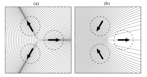
Figure 3: Lines indicating the directions of maximum fluctuations in the transverse magnetization for the half-quantum vortex state in Eq. (26), where (a) and (b) correspond to the $+$ and $-$ signs, respectively. The dashed circles show schematics of the threefold domains and the arrows show the directions of magnetization in the domains.

Spontaneous magnetization tends to occur in the directions of large spin fluctuations, i.e., the directions of the lines in Fig. 3. For spontaneous magnetization, the total magnetization $\int d\bm{r}\bm{F}$ must be conserved. From these two constraints, we understand the reason for the threefold domain formation. The arrows in Fig. 3 show examples of transverse magnetization satisfying the two constraints, where the magnetization in each domain occurs in the direction of the line and the sum of the three magnetization vectors vanishes.

We note that continuous magnetization for all $\theta$, as in the polar-core and Mermin-Ho vortices, is impossible, since the symmetry group of the ferromagnetic state is different from that of the spin state in Eq. (26). The half-quantum vortex structure is peculiar to the latter symmetry group. Twofold domain formation is also impossible, since spin directions at $\theta$ and $\theta+\pi$ differ by $\pi/2$ (not $\pi$) and the total spin is not conserved.

For $j$-fold domain formation, the center of each domain is located at $\theta=2\pi p/j$ with $p=0,1,\cdots,j-1$. For each domain, there are two possible directions of magnetization, $\mp\pi p/j$ and $\mp\pi p/j+\pi$, where the $\mp$ signs correspond to the $\pm$ signs in Eq. (26). For the spin conservation to be satisfied, the sum of these magnetization vectors must vanish:

$$\sum_{p=0}^{j-1}\left(e^{\mp i\pi p/j}\;\;\;{\rm or}\;\;\;e^{\mp i(\pi p/j+\pi)}\right)=0.$$ (29)

For $j=1$ and $2$, Eq. (29) cannot be satisfied. For $j=3$, we find $1+e^{\mp i(\pi/3+\pi)}+e^{i2\pi/3}=0$, which corresponds to the arrows in Fig. 3. In general, Eq. (29) can only be satisfied for an odd $j\geq 3$. This result agrees with that in Sec. IV.2.

VI Conclusions

We have studied the dynamics of spontaneous magnetization of a half-quantum vortex state in a spin-1 BEC with a ferromagnetic interaction. Solving the GP equation numerically, we found that the axisymmetry is spontaneously broken and the threefold magnetic domains are formed through the dynamical instability (Fig. 1). The critical strength of the interaction for the dynamical instability was obtained by the Bogoliubov analysis (Fig. 2). In order to understand the phenomenon in an analytic manner, we investigated the 1D ring model and showed that the transverse magnetization is most unstable against forming the threefold domains among the $j$-fold domains with odd integers $j\geq 3$ (Sec. IV.2). We provided a physical interpretation of the phenomenon based on the topological spin structure of the half-quantum vortex and spin conservation (Fig. 3).

The half-quantum vortex in a spin-1 BEC is peculiar to the symmetry group that the spin state (26) possesses. For the ferromagnetic interaction, in which the state (26) is unstable, the system exhibits nontrivial dynamics, namely, threefold domain formation. We expect that various pattern formation phenomena may occur in magnetic phase transitions in spinor BECs containing topological structures, in which the symmetry groups of the spin states change in the phase transitions.

References

• (1) N. D. Mermin and T. -L. Ho, Phys. Rev. Lett. 36, 594 (1976).
• (2) P. W. Anderson and G. Toulouse, Phys. Rev. Lett. 38, 508 (1977).
• (3) A. E. Leanhardt, Y. Shin, D. Kielpinski, D. E. Pritchard, and W. Ketterle, Phys. Rev. Lett. 90, 140403 (2003).
• (4) A. E. Leanhardt, A. Görlitz, A. P. Chikkatur, D. Kielpinski, Y. Shin, D. E. Pritchard, and W. Ketterle, Phys. Rev. Lett. 89, 190403 (2002).
• (5) L. E. Sadler, J. M. Higbie, S. R. Leslie, M. Vengalattore, and D. M. Stamper-Kurn, Nature (London) 443, 312 (2006).
• (6) G. E. Volovik and V. P. Mineev, JETP Lett. 24, 561 (1976).
• (7) U. Leonhardt and G. E. Volovik, JETP Lett. 72, 46 (2000).
• (8) F. Zhou, Phys. Rev. Lett. 87, 080401 (2001).
• (9) U. A. Khawaja and H. Stoof, Nature (London) 411, 918 (2001); Phys. Rev. A 64, 043612 (2001).
• (10) Y. Kawaguchi, M. Nitta, and M. Ueda, Phys. Rev. Lett. 100, 180403 (2008); ibid. 101, 029902(E) (2008).
• (11) T.-L. Ho, Phys. Rev. Lett. 81, 742 (1998).
• (12) M. F. Andersen, C. Ryu, P. Cladé, V. Natarajan, A. Vaziri, K. Helmerson, and W. D. Phillips, Phys. Rev. Lett. 97, 170406 (2006).
• (13) H. Saito, Y. Kawaguchi, and M. Ueda, Phys. Rev. Lett. 96, 065302 (2006).
• (14) H. Schmaljohann, M. Erhard, J. Kronjäger, M. Kottke, S. van Staa, L. Cacciapuoti, J. J. Arlt, K. Bongs, and K. Sengstock, Phys. Rev. Lett. 92, 040402 (2004).
• (15) E. G. M. van Kempen, S. J. J. M. F. Kokkelmans, D. J. Heinzen, and B. J. Verhaar, Phys. Rev. Lett. 88, 093201 (2002).
• (16) T. Isoshima, K. Machida, and T. Ohmi, J. Phys. Soc. Jpn 70, 1604 (2001).
• (17) J. Ruostekoski and J. R. Anglin, Phys. Rev. Lett. 91, 190402 (2003).
• (18) A.-C. Ji, W. M. Liu, J. L Song, and F. Zhou, Phys. Rev. Lett. 101, 010402 (2008).
• (19) H. Chiba and H. Saito, arXiv:0806.3840.
• (20) J. L. Song and F. Zhou, arXiv:0806.2323.
• (21) H. Saito, Y. Kawaguchi, and M. Ueda, Phys. Rev. A 75, 013621 (2007).
• (22) H. Saito, Y. Kawaguchi, and M. Ueda, Phys. Rev. A 76, 043613 (2007).
• (23) J. M. Higbie, L. E. Sadler, S. Inouye, A. P. Chikkatur, S. R. Leslie, K. L. Moore, V. Savalli, and D. M. Stamper-Kurn, Phys. Rev. Lett. 95, 050401 (2005).
• (24) M. Edwards, R. J. Dodd, C. W. Clark, and K. Burnett, J. Res. Natl. Inst. Stand. Technol. 101, 553 (1996).