Thermodynamic Properties of ^56,57Fe

Abstract

Nuclear level densities for ^56,57Fe have been extracted from the primary $\gamma$-ray spectra using (³He,³He${}^{\prime}\gamma$) and (³He,$\alpha\gamma$) reactions. Nuclear thermodynamic properties for ⁵⁶Fe and ⁵⁷Fe are investigated using the experimental level densities. These properties include entropy, Helmholtz free energy, caloric curves, chemical potential, and heat capacity. In particular, the breaking of Cooper pairs and single-quasiparticle entropy are discussed and shown to be important concepts for describing nuclear level density. Microscopic model calculations are performed for level densities of ^56,57Fe. The experimental and calculated level densities are compared. The average number of broken Cooper pairs and the parity distribution are extracted as a function of excitation energy for ^56,57Fe from the model calculations.

I Introduction

Nuclear thermodynamics has attracted considerable attention in recent years. Several temperature-dependent nuclear properties such as nuclear shapes, giant dipole resonance widths and their fluctuation properties have been investigated in the literature kusnezov1998 . In this context one of the most interesting topics is that of phase transitions in atomic nuclei. Different types of phase transitions have been discussed in nuclear physics. One is the first order phase transition in the multifragmentation of nuclei which occurs at high temperatures dagostino1996 . Negative heat capacities observed in multifragmentation of nuclei have been obtained from energy fluctuations and interpreted as an indicator of a first order phase transition dagostino1996 ; chomaz2000 .

The second type of phase transition in atomic nuclei is the transition from a phase with strong pairing correlations to a phase with weak pairing correlations sano1963 . The onset of a discontinuity in thermodynamic variables and the evolution of zeros of the canonical sumaryada2007 ; schiller2002a and grand-canonical partition functions schiller2002a in the complex plane have been discussed in terms of pairing transitions.

Recently kaneko2007 , thermal properties for ⁵⁶Fe have been calculated using both static-path approximation (SPA) and SPA plus random-phase approximation (RPA). These calculations show that the increase of the moment of inertia with increasing temperature is correlated with the suppression of pairing correlations.

Furthermore, structures in the heat-capacity curve related to the quenching of pairing correlations have been obtained within relativistic mean field theory agrawal2001 , the finite-temperature Hartree-Fock-Bogoliubov theory egido2000 , and the shell-model Monte Carlo (SMMC) approach liu2001 . An $S$-shaped structure in the heat capacity curve derived from the level densities of low-spin states has also been observed experimentally schiller2001 and interpreted as a signature of a pairing phase transition.

As a part of an ongoing effort, in the present work we extract several thermodynamic properties of ⁵⁶Fe and ⁵⁷Fe isotopes starting from nuclear level densities. Details of the experiment, analysis tools, the Oslo method, and experimental level densities are presented in Sect. II. Thermodynamic concepts are discussed in Sect. III and comparison with a combinatorial model is shown in Sect. IV. Finally our results are summarized in Sect. V.

II Experimental details and data analysis

The self-supporting ⁵⁷Fe target was bombarded by a 2-nA beam of 45-MeV ³He particles from the Oslo Cyclotron Laboratory at the University of Oslo. The target was isotopically enriched to 94.7%, and had a thickness of 3.4 mg/cm². The outgoing charged particles were recorded by eight Si $\triangle$E-E telescopes, which were collimated and placed 5 cm away from the target at a ring located at 45^∘ with respect to the beam direction. The particle telescopes covered 0.3% of the total solid angle. The thicknesses of the front and the end detectors were 140 and 3000 $\mu$m, respectively, and the particle energy resolution was $\approx$ 0.3 MeV over the entire spectrum. The reaction $\gamma$ rays were detected by 28 collimated 5^′′ x 5^′′ NaI(Tl) detectors with a total efficiency of $\approx$ 15% of 4$\pi$, and with 6% energy resolution at 1.3 MeV. In order to monitor the selectivity and populated spin distribution of the reactions, one 60% Ge(HP) detector was used.

The excitation energy of the final nucleus is determined from the known $Q$ value and the reaction kinematics using particle-$\gamma$ coincidence information. A total $\gamma$-ray spectrum is obtained for each excitation energy region. These $\gamma$-ray spectra are then unfolded using a Compton subtraction method guttormsen1996 . A two-dimensional primary $\gamma$-ray matrix is extracted by applying a subtraction method to the unfolded $\gamma$-ray spectra guttormsen1987 . Basic assumptions and details of the subtraction method are given in Ref. guttormsen1987 .

The primary $\gamma$-ray matrix is factorized using the Brink-Axel hypothesis brink ; axel1962 , according to which the probability of emitting a $\gamma$ ray from an excited state is proportional to the $\gamma$-ray transmission coefficient $\mathcal{T}(E_{\gamma})$ and the level density at the final energy $\rho(E-E_{\gamma})$. This factorization is determined by a least $\chi^{2}$ method without assuming any functional form for the level density and the $\gamma$-ray transmission coefficient schiller2000 . However, this method does not provide a unique solution. This factorization is invariant under the transformation schiller2000

$${\tilde{\rho}}(E-E_{\gamma}) = A\exp(\alpha(E-E_{\gamma}))\rho(E-E_{\gamma})$$

$${\tilde{\cal T}}(E_{\gamma}) = B\exp(\alpha E_{\gamma}){\cal T}(E_{\gamma}),$$ (1)

where $A$, $B$, and $\alpha$ are the free parameters of the transformation. Therefore it is very important to determine accurately the free parameters $A$, $B$, and $\alpha$ in order to find the physical solution. The parameters $A$ and $\alpha$ are determined from the normalization of the level density to the discrete levels at low excitation energies and to the density of the neutron resonances at the neutron binding energy $B_{n}$. The parameter $B$ is then determined using the average total radiative width of neutron resonances voinov2001 .

Since there are no neutron resonance data for the ⁵⁶Fe compound nucleus a different procedure for the normalization of the level density is performed. We use ⁵⁷Fe as a basis, since both average neutron resonance spacings $D$ and total radiative widths $\Gamma_{\gamma}$ of neutron resonances are well known mughabghab . The procedure for extracting the total level density $\rho(B_{n})$ from the average resonance spacing $D$ is described in Ref. schiller2000 . Then we apply the von Egidy and Bucurescu parameterization of the back-shifted Fermi gas formula egidy2005

$$\rho_{\mathrm{B}SFG}=\eta\frac{\exp(2\sqrt{aU})}{12\sqrt{2}a^{1/4}U^{5/4}\sigma},$$ (2)

where $a$ is the level density parameter, and the intrisic excitation energy $U=E-E_{1}$ is determined by the backshift parameter $E_{1}$. In this global description of the level density, shell corrections are taken into account in the estimation of the $a$ and $E_{1}$ parameters egidy2005 . By fitting $\rho_{\mathrm{B}SFG}$ to $\rho(B_{n})$ in ⁵⁷Fe, we determine the normalization parameter $\eta=0.852$ of Eq. (2). This value is then adopted for ⁵⁶Fe together with the prescribed $a$ and $E_{1}$ parameters. The parameters used are listed in Table 1.

Figure 1 shows the level densities of ^56,57Fe from the ground state up to $E$ $\sim$ $B_{n}-1$ MeV. They are normalized to discrete levels at low excitation energies (jagged lines) and to the level densities at the neutron binding energy $B_{n}$ (triangles). The arrows indicate the fitting regions used. As described above, the triangles are determined from Eq. (2) with $\eta=0.852$ for ⁵⁶Fe and from the observed $D$ value for ⁵⁷Fe.

Figure 1: (a) Experimental level density of ⁵⁶Fe (full circles). The jagged solid lines represent the level density obtained from counting of discrete levels firestone . The smooth solid curve is the renormalized level density parametrization according to von Egidy and Bucurescu egidy2005 . The data points between the arrows at low and high excitations are used for the normalization. The triangle at $B_{n}$ is determined from $\rho_{\mathrm{B}SFG}$ with $\eta=0.852$. The level density obtained from the ⁵⁵Mn(d,n)⁵⁶Fe reaction voinov2006 (open circles) is scaled with a factor of 1.3. (b) Experimental level density of ⁵⁷Fe (full circles). The triangle at $B_{n}$ is determined from neutron resonance spacings. The level density obtained from the ⁵⁸Fe(³He,$\alpha$)⁵⁷Fe reaction voinov2007 (open circles) is scaled with a factor of 2.6.

The level density obtained with the Oslo method follows well that obtained by counting of discrete levels up to around 5 and 2.5 MeV of excitation energies in ^56,57Fe, respectively. Both nuclei show an abrupt increase in level density at $E=2-3$ MeV, indicating the first breaking of nucleon Cooper pairs.

Figure 1 also includes level densities from particle evaporation data (open circles) measured with the ⁵⁵Mn(d,n)⁵⁶Fe reaction voinov2006 , and with the ⁵⁸Fe(³He,$\alpha$)⁵⁷Fe and ⁵⁹Co($d,\alpha$)⁵⁷Fe reactions voinov2007 . The method determines the slope of the level densities, but not the absolute normalization constant. Thus, these data have been scaled to match $\rho_{\mathrm{B}SFG}$ (solid smooth curves). The slopes of the level densities from evaporation studies fit very well with the employed $\rho_{\mathrm{B}SFG}$. This gives support to the level density parameters $a$ extracted as prescribed in Ref. egidy2005 and listed in Table 1.

From Eq. (1) we see that the $\alpha$ parameter determines the slope of the transmission coefficient, and thereby also the radiative strength function (RSF) $f(E_{\gamma})=\mathcal{T}(E_{\gamma})/(2\pi E_{\gamma}^{3})$, assuming only dipole radiation. The RSFs have been published previously voinov2004 ; voinov2006 , but with other normalization procedures. Thus, for completeness, we show in Fig. 2 the renormalized RSFs. In the ⁵⁷Fe case, the $B$ parameter of Eq. (1) was determined from the average radiative width $\langle\Gamma_{\gamma}\rangle$ of neutron resonances at $B_{n}$ mughabghab . For ⁵⁶Fe, where no $\langle\Gamma_{\gamma}\rangle$ exists, we scale the total RSF to match ⁵⁷Fe. The parameters are listed in Table 1.

Figure 2: Radiative strength functions for ⁵⁶Fe and ⁵⁷Fe.

Table 1: Back-shifted Fermi gas level density parameters and normalization constants.

Isotope	$B_{n}$	a	$E_{1}$	$D$	$\sigma(B_{n})$	$\eta$	$\rho(B_{n})$	$\langle\Gamma_{\gamma}\rangle$
	(MeV)	(MeV-1)	(MeV)	(keV)			(MeV-1)	(meV)
56Fe	11.197	6.196	0.942	2.6(6)a	4.049	0.852a	3600(800)a	2300(1200)a
57Fe	7.646	6.581	-0.523	22.0(17)	3.834	0.852	1380(170)	900(470)

^a Based on systematics, see text.

III Thermodynamic quantities

Depending on the system under study, one can chose among different kinds of statistical ensembles in order to derive thermodynamic quantities. The thermodynamic quantities derived within different ensembles give the same results in the thermodynamic limit. On the other hand, the choice of a specific ensemble may change results significantly for small systems. For example, the caloric curves derived within the microcanonical and canonical ensembles coincide for large systems; but the two caloric curves depart from each other for small systems schiller2005 ; tavukcu .

The microcanonical ensemble is commonly accepted as the appropriate ensemble to use in investigating atomic nuclei, as the nuclear force has a short range and the nucleus does not share its excitation energy with its surroundings. However some thermodynamic quantities such as temperatures and heat capacities may have large fluctuations and negative values when derived within the microcanonical ensemble. On the other hand, the canonical ensemble averages too much over structural changes of the system. Therefore, it is diffucult to chose an appropriate ensemble for a small system. Here, we use both microcanonical and canonical ensembles to study the thermodynamic properties of the system.

III.1 Microcanonical Ensemble

The microcanonical entropy is closely related to the level density of the system at a given excitation energy. Several thermodynamic properties of the atomic nucleus can be derived from the entropy. The entropy is defined as the natural logarithm of the multiplicity $\Omega$ of accessible states within the energy interval $E$ and $E+\delta E$:

$$S(E)=k_{B}\ln\Omega(E),$$ (3)

where $k_{B}$ is the Boltzmann’s constant. Here we set $k_{B}$ to unity so that the entropy becomes dimensionless and thus the temperature $T$ has the unit of MeV. One should note that the experimental level density is not the true multiplicity of states; i.e., it does not include the $(2I+1)$ degeneracy of magnetic substates. Thus, in order to obtain the state density $\Omega$, one needs to know the spin distribution as a function of excitation energy. The spin distribution is usually assumed to be Gaussian with a mean of $\langle 2I+1\rangle=\sqrt{2\pi}\sigma$, where $\sigma$ is the spin cut-off parameter which depends very weakly ($\sigma\propto E^{1/4}$) on excitation energy.

However, in this work we define a “pseudo” entropy based on the experimental level density, i.e., $\Omega(E)=\rho(E)/\rho_{0}$. The normalization constant $\rho_{0}$ is introduced and adjusted such that the third law of thermodynamics is fulfilled as $S(T\rightarrow 0)=0$. The ground states of even-even nuclei represent a well-ordered system with no thermal excitation and are characterized by zero entropy and temperature. Therefore the normalization constant is set to $\rho_{0}=$ 1 MeV^-1 in order to obtain $S=\ln\Omega\sim 0$ in the ground state band region of ⁵⁶Fe. The extracted $\rho_{0}$ is also used for the ⁵⁷Fe nucleus.

Figure 3 shows the entropies of ^56,57Fe. The breaking of the first Cooper pair appears in the $E=2-3$ MeV excitation energy region for both nuclei, indicating a slightly delayed breaking for ⁵⁷Fe due to the odd valence neutron.

Figure 3: Upper panel: Deduced entropies for ^56,57Fe. The solid line is the constant temperature least square fit to the data. Lower panel: Deduced entropy excess for the single particle calculated using Eq. (5). The entropy excess is $\Delta S=1.2(4)$.

The entropies of ^56,57Fe appear fairly linear at high excitation energies, and the slope of the entropy is related to the temperature of the system by

$$T=(dS/dE)^{-1}_{V}.$$ (4)

The entropies of ^56,57Fe are fit with a constant temperature model, shown with solid lines in Fig. 3. From this model, constant temperatures of $T=1.2(3)$ MeV and $T=1.0(3)$ MeV are found for ⁵⁶Fe and ⁵⁷Fe, respectively. These temperatures are interpreted as the critical temperatures $T_{c}$ for the breaking of nucleon pairs.

The entropy difference between the even-odd and even-even nuclei is interpreted as the entropy of a single quasiparticle (particle or hole), assuming that the entropy is an extensive (additive) quantity. The entropy carried by the valence neutron particle in our case can be estimated by

$$\Delta S=S(^{57}\text{Fe})-S(^{56}\text{Fe}).$$ (5)

The lower panel of Fig. 3 shows the single particle entropy as a function of excitation energy. The fluctuations at the low excitation energies result from the lower pairing gap in the odd-mass system. At higher excitation energies above $\sim$ 4 MeV, the entropy difference has a relatively constant value, revealing the statistical behavior of these isotopes, $\Delta S=1.2(4)$. This value is less than the value obtained for the rare-earth isotopes which is $\Delta S=1.7$ guttormsen2001-2 . This is expected because ⁵⁶Fe and ⁵⁷Fe isotopes are in the vicinity of closed shells, thus the entropy is less than that of the rare-earth isotopes.

Assuming a constant $\Delta S$ and a constant energy shift $\Delta$ between the two entropies, these two quantities are connected to the critical temperature $T_{c}$ guttormsen2001-2 by

$$T_{c}=\frac{1}{\Delta S}\Delta.$$ (6)

From this relation, we can calculate the entropy difference $\Delta S=\Delta/T_{c}=1.5/1.1\sim 1.4$, which is consistent with the present observations. Here, the gap parameter $\Delta$ is assumed to include both the pairing gap and the contribution from the distance between the Fermi surface and the closest neutron orbital.

III.2 Canonical Ensemble

In a canonical ensemble, a physical system is in thermal equilibrium with a heat reservoir at constant temperature and can exchange energy (but not particles) with the reservoir. Analogous to the entropy in the microcanonical ensemble, the partition function is the starting point to obtain the thermodynamics of a system in the canonical ensemble. The partition function for a given temperature is determined by

$$Z(T)=\sum_{E=0}^{\infty}\rho(E)\delta Ee^{-E/T},$$ (7)

where $\rho(E)$ is the measured level density, and $\delta E$ is the energy bin used. The summation in $Z(T)$ goes to infinity and our level densities extend to $\sim B_{n}-1$ MeV. Therefore we extrapolate the experimental level densities using the BSFG model parameterized by von Egidy and Bucurescu egidy2005 . The Helmholtz free energy can be calculated from the partition function by

$$F(T)=-T\ln Z(T).$$ (8)

This equation gives the connection between statistical mechanics and thermodynamics in the canonical ensemble, as does the entropy in the microcanonical ensemble. Then the entropy $S$, the average excitation energy $\langle E\rangle$, the heat capacity $C_{V}$, and the chemical potential $\mu$ at a given temperature can be derived from $F(T)$ by

$$S(T)=-\left(\frac{\partial F}{\partial T}\right)_{V},$$ (9)

$$\langle E(T)\rangle=F+TS,$$ (10)

$$C_{V}(T)=\left(\frac{\partial\langle E\rangle}{\partial T}\right)_{V},$$ (11)

$$\mu(T)=\frac{\partial F}{\partial n},$$ (12)

where $n$ is the number of thermal particles. These thermal particles outside a core of Cooper pairs are responsible for the thermal properties of the nucleus at low excitations. At higher temperatures, pairing correlations are quenched, and the nucleus has a transition from a paired to unpaired phase.

Figure 4: The Helmholtz free energy $F$, average excitation energy $\langle E(T)\rangle$, entropy S, and heat capacity C_V for ⁵⁶Fe (dashed lines) and ⁵⁷Fe (solid lines), deduced in the canonical ensemble.

Figure 5: The experimental Helmholtz free energies deduced in the canonical ensemble for ⁵⁶Fe and ⁵⁷Fe. The critical temperature for the quenching of pairing correlations is indicated by $T_{c}$, where the chemical potential is $\mu\sim 0$.

Figure 4 shows the Helmholtz free energy $F$, average excitation energy $\langle E(T)\rangle$, entropy $S$, and heat capacity C_V for ⁵⁶Fe (dashed lines) and ⁵⁷Fe (solid lines). The Helmholtz free energy $F$ and the average excitation energy $\langle E(T)\rangle$ behave smoothly as a function of temperature. At around $T\sim 1.3$ MeV, both isotopes are excited to energies comparable to their respective neutron binding energies. Average excitation energies for ⁵⁶Fe and ⁵⁷Fe coincide only at one point $T\sim 2$ MeV. Above this temperature the odd isotope has larger values as the temperature increases. The entropy $S$ and heat capacity C_V are the first and second derivatives of $F$, respectively, and thus both reflect thermal variations. For temperatures below $T=1$ MeV, the entropy difference for ⁵⁶Fe and ⁵⁷Fe reaches $\sim 2$, the entropy of ⁵⁷Fe being larger. The entropies have similar values for $T=1-1.5$ MeV. Above $T=1.5$ MeV, the two entropies start to diverge. Both heat capacities have an $S$ shape which is interpreted as a fingerprint for pairing transitions in nuclei. The structure in the heat capacity C_V for ⁵⁷Fe is more pronounced than the C_V for ⁵⁶Fe, which is the opposite of what SMMC calculations predict. The contribution to the heat capacity from collective excitations is negligible, and has no influence on the $S$ shape guttormsen2001 .

Figure 5 shows the chemical potential ${\mu}$ which is defined as the amount of energy required to excite a nucleon from the underlying core of paired nucleons, while the entropy and volume held fixed. The typical energy cost for creating a quasiparticle is $-\Delta$ which is also equal to the chemical potential. The chemical potential can be written as

$$\mu=\frac{\Delta F}{\Delta N}=\frac{F_{odd}-F_{even}}{1}=-\Delta.$$ (13)

thus giving $F_{even}=F_{odd}+\Delta$. The energy curve of ⁵⁷Fe can be interpreted as the free energy for an even-even system with one extra nucleon.

III.3 Probability Density Functions

An alternative way of studying the energy-temperature relation of a system is the probability density function, which is the probability of the system having energy $E$ for a given temperature, and is given by

$$P(E)=\frac{\Omega(E)\exp(-E/T)}{Z(T)}.$$ (14)

In the thermodynamic limit $P(E)$ is very sharp - similar to a $\delta$ function. However, for small systems the multiplicity of states is much smaller, which makes the probability distribution broader. Figure 6 shows the probability density functions for ^56,57Fe nuclei for various temperatures. Below $T\sim 1$ MeV, the distribution is mainly based on the experimental level density. For increasing temperatures, the energy of the nucleus increases; therefore, the probability density function depends more and more on the extrapolated level density.

Below $T=1.2$ MeV, the distribution is slightly broader for ⁵⁶Fe due to collective excitations below the pairing gap in this nucleus. The effect of critical temperatures obtained with the constant temperature least-square fit can also be seen on the probability density function. At $T_{c}=1.2$ MeV and $T_{c}=1.0$ MeV for ^56,57Fe, respectively, the probability distribution becomes broader where the breaking of nucleon pair process is strongest.

Figure 6: Observed probability density functions for ^56,57Fe for various temperatures.

IV Comparison of level densities with microscopic calculations

In order to extract more information on the underlying nuclear structure resulting in the observed level density, we have performed microscopic calculations with the code micro larsen_Sc . The code is based on a model employing Bardeen-Cooper-Schrieffer (BCS) quasiparticles BCS , which are distributed on all possible proton and neutron configurations according to the given excitation energy $E$ of the nucleus. The advantage of this code is a fast algorithm that may include a large model space of single-particle states. Since level density is a gross property, the detailed knowledge of the many-particle matrix elements through large diagonalizing algorithms is not necessary.

The single-particle energies $e_{\rm sp}$ are calculated with the Nilsson Hamiltonian for an axially deformed core with a quadrupole deformation parameter $\epsilon_{2}$. The spin-orbit and centrifugal parameters $\kappa$ and $\mu$, together with the oscillator quantum energy $\hbar\omega_{0}=41A^{-1/3}$ MeV between the harmonic oscillator shells, are also input to the code. Within the BCS model, the single-quasiparticle energies are defined by

$$e_{\rm qp}=\sqrt{(e_{\rm sp}-\lambda)^{2}+\Delta^{2}},$$ (15)

where the Fermi level $\lambda$ is adjusted to reproduce the number of particles in the system and $\Delta$ is the pair-gap parameter.

In the calculations we have adopted the Nilsson parameters $\kappa=0.066$ and $\mu=0.32$ taken from Ref. white . The quadrupole deformation $\epsilon_{2}$ was set to 0.24 for ⁵⁶Fe, and 0.25 for ⁵⁷Fe RIPL . The Nilsson levels used in the calculations for ⁵⁶Fe are shown in Fig. 7, with the Fermi levels for the protons and neutrons.

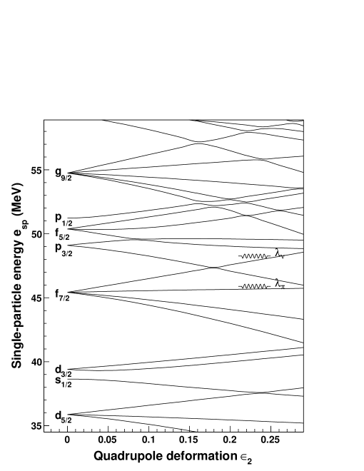
Figure 7: Nilsson level scheme for ⁵⁶Fe.

The rotational and vibrational terms, which are schematically added, contribute significantly to the total level density only in the lower excitation region. The rotational parameter $A_{\rm rot}$ was set to $0.12$ MeV in order to reproduce the ground-state rotational band of ⁵⁶Fe firestone . The adopted pairing gap parameters $\Delta_{\pi}$ and $\Delta_{\nu}$ were evaluated from even-odd mass differences Wapstra according to Ref. BM (see Table 2 for a list of all parameters used).

Table 2: Input parameters for the model calculations.

Isotope	$\epsilon_{2}$	$\Delta_{\pi}$	$\Delta_{\nu}$	$A_{\rm rot}$	$\hbar\omega_{0}$	$\hbar\omega_{\rm vib}$	$\lambda_{\pi}$	$\lambda_{\nu}$
		(MeV)	(MeV)	(MeV)	(MeV)	(MeV)	(MeV)	(MeV)
56Fe	0.24	1.568	1.363	0.120	10.65	2.656	45.89	48.23
57Fe	0.25	1.268	1.465a	0.120	10.72	2.656	45.66	48.40

^a Taken from ⁵⁸Fe.

The experimental and calculated level densities for ^56,57Fe are shown in Fig. 8. In general, there is a very good overall agreement between the measured level densities and the calculations, even without reducing the pairing gap. This is in contradiction with what is usually thought using the canonical ensemble. However, excitation energy around 8 MeV may be too low to see the overall quenching of the pairing correlations demonstrated in Figs. (4) and (5). Microcanonical and canonical ensembles yield different results for small systems. It is, therefore, no surprise that one measures different thermodynamic quantities within these ensembles.

In Fig. 8, especially for ⁵⁶Fe, it is gratifying how both the general functional form and the absolute magnitude of the level densities are reproduced. In the case of ⁵⁷Fe, there is an overshoot in the calculated level density compared to the experimental data from about 3.5 MeV excitation energy. This excess could be due to the neutron $f_{5/2}$, $p_{1/2}$ and $g_{9/2}$ orbitals coming into play too soon, that is, they are too close to the neutron Fermi level. Another possibility is that the adopted (constant) deformation is too large at these excitation energies, where it may be that the nuclear structure favors a more spherical shape.

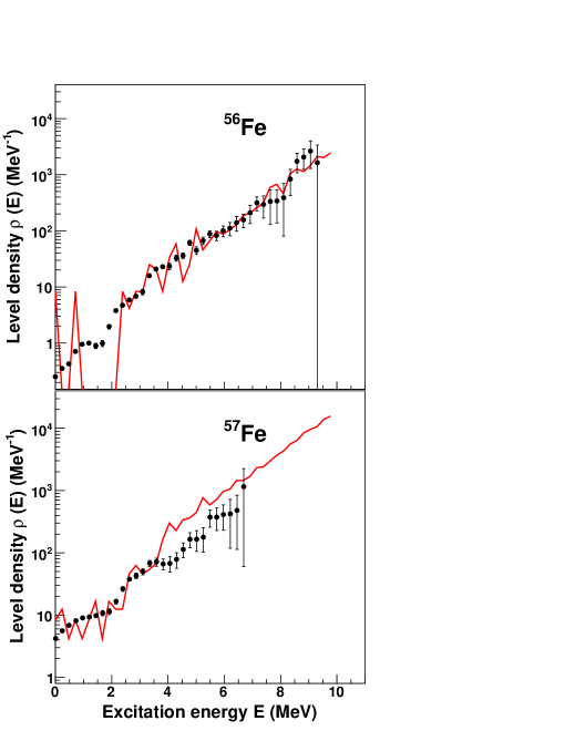
Figure 8: Calculated level densities (solid line) compared with the experimental ones (data points with error bars) for ^56,57Fe.

Figure 9 shows the average number of broken Cooper pairs $\langle N_{\mathrm{qp}}\rangle$ as a function of excitation energy. Both neutron and proton pairs are taken into account, adding up to the total number of broken pairs. From Fig. 9, the pair-breaking process is seen to start at $E\approx 2.5$ MeV for both nuclei, in accordance with the values used for the pair-gap parameters (see Table 2).

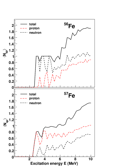
Figure 9: The average number of broken Cooper pairs as a function of excitation energy for ^56,57Fe.

A prominent step structure at $\langle N_{\mathrm{qp}}\rangle=1$ is seen clearly in ⁵⁶Fe for excitation energies between $2.5\leq E\leq 5.5$ MeV, and for ⁵⁷Fe in the energy region $4.0\leq E\leq 7.5$ MeV. This means that on average there is one Cooper pair broken, which could be either a proton or a neutron pair. For ⁵⁶Fe, the total $\langle N_{\mathrm{qp}}\rangle$ exhibits an increase for $E>5.5$ MeV up to about 9 MeV, where there seems to be a saturation for $\langle N_{\mathrm{qp}}\rangle\approx 2$. This is also reflected in the proton and neutron contributions to $\langle N_{\mathrm{qp}}\rangle$. A similar behavior can be seen in ⁵⁷Fe for excitation energies higher than $\approx 8$ MeV. We observe that the onset of this increase is at higher excitation energies than for ⁵⁶Fe. A possible explanation of this is that the ⁵⁷Fe valence neutron blocks the quasi-particles created during the pair-breaking process, suppressing the average number of quasi-particles even at high excitation energies. This is supported by the fact that the neutron contribution to the total $\langle N_{\mathrm{qp}}\rangle$ is lower or about the same as the proton contribution in ⁵⁷Fe, while in ⁵⁶Fe, the neutron contribution is in general higher than the proton contribution.

The present model gives the opportunity of investigating the parity distribution as a function of excitation energy. For this purpose, we utilize the parity asymmetry defined in Ref. gary by

$$\alpha=\frac{\rho_{+}-\rho_{-}}{\rho_{+}+\rho_{-}},$$ (16)

which becomes $-1$ if only negative parity states are present, $+1$ if there are only positive parity states, and 0 when both parities are equally represented. In literature, one also find the expression $\rho_{-}/\rho_{+}$ which relates to $\alpha$ by

$$\frac{\rho_{-}}{\rho_{+}}=\frac{1-\alpha}{1+\alpha}.$$ (17)

The parity asymmetry $\alpha$ for ^56,57Fe is shown in Fig. 10.

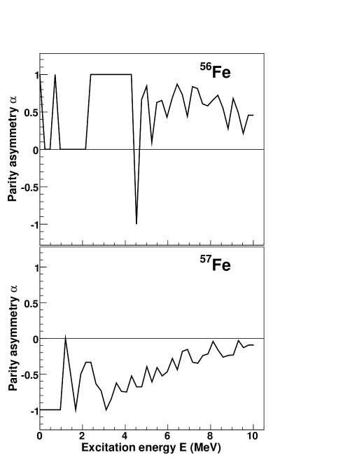
Figure 10: The parity asymmetry as function of excitation energy for ^56,57Fe.

From Fig. 10, we see that there is an excess of positive parity states in ⁵⁶Fe and negative parity states in ⁵⁷Fe. As the excitation energy increases, the parity asymmetry decreases for both nuclei, and shows an almost decay-like behavior, especially in the case of ⁵⁷Fe. Here, the parity asymmetry is close to zero at $E=9-10$ MeV. For ⁵⁶Fe, there is still a significant overshoot of positive-parity states in this energy region, giving an average parity asymmetry of $\alpha\approx 0.35$ for $9.5\simeq E\simeq 10$ MeV.

We have compared our results with the shell-model Monte Carlo results of Y. Alhassid et al. Alhassid , and with recent macroscopic-microscopic calculations performed by D. Mocelj et al. Rauscher . In Fig. 2 of Ref. Rauscher , the ratio $\rho_{-}/\rho_{+}$ is shown for ⁵⁶Fe, indicating a value of $\rho_{-}/\rho_{+}\simeq 0.1$ at 10 MeV excitation energy. From Fig. 4 in Ref. Alhassid , the ratio $\rho_{-}/\rho_{+}\simeq 0.2$ for $E=10$ MeV. Using an average parity asymmetry of $\alpha\approx 0.35$ as determined in the previous section, we obtain $\rho_{-}/\rho_{+}\approx 0.5$, which implies a considerable number of additional positive-parity states than predicted by the macroscopic-microscopic model and the shell-model Monte Carlo approach. For ⁵⁷Fe with $\alpha\approx 0.1$ for $9.5\simeq E\simeq 10$ MeV, we find $\rho_{-}/\rho_{+}\approx 0.8$. However, one should note that in our calculations, the parity asymmetry strongly depends on the position of the neutron $g_{9/2}$ orbital relative to the Fermi level (see Fig. 7).

V Summary

Nuclear level densities for ^56,57Fe are renormalized using the new level density parameterization suggested by von Egidy and Bucurescu. The level densities obtained with the Oslo method agree well with those obtained from other experiments. The experimental level densities are used to extract thermodynamic quantities. The entropies for ^56,57Fe obtained in the microcanonical ensemble reveal step structures indicating the breaking of nucleon Cooper pairs. The entropy carried by the single neutron at higher excitation energies (4 MeV $<E<$ 7 MeV) is estimated to be $\Delta S=1.2(4)k_{B}$ which is smaller than that of the rare-earth isotopes.

Assuming a constant $\Delta S$, a critical temperature for the depairing process was determined. In the canonical ensemble, several thermodynamic properties were investigated. Probability density functions for ^56,57Fe were also extracted which reveal the difference between small systems such as the atomic nucleus and a system in the thermodynamic limit.

Microscopic model calculations based on BCS quasiparticles were performed. The overall agreement between the experimental and calculated level densities are good. Step structures observed in the experimental level densities are also observed in the plot of the average number of broken pairs as a function of excitation energy. The parity distributions obtained from model calculations for ^56,57Fe indicate a decrease of parity asymmetry for both isotopes as the excitation energy increases. The microscopic model, which is expressed within the microcanonical ensemble (fixed $E$ with no heat bath), describes the observed level densities without the need of attenuation of the pairing-gap energies for excitation energies below 8 MeV.