The effects of Gribov copies in $2D$ gauge theories

Abstract

In previous works, we have shown that the Gribov-Zwanziger action, which implements the restriction of the domain of integration in the path integral to the Gribov region, generates extra dynamical effects which influence the infrared behaviour of the gluon and ghost propagator in $SU(N)$ Yang-Mills gauge theories. The latter are in good agreement with the most recent lattice data obtained at large volumes, both in $4D$ and in $3D$. More precisely, the gluon propagator is suppressed and does not vanish at zero momentum, while the ghost propagator keeps a $1/p^{2}$ behaviour for $p^{2}\approx 0$. Instead, in $2D$, the lattice data revealed a vanishing zero momentum gluon propagator and an infrared enhanced ghost, in support of the usual Gribov-Zwanziger scenario. We will now show that the $2D$ version of the Gribov-Zwanziger action still gives results in qualitative agreement with these lattice data, as the peculiar infrared nature of $2D$ gauge theories precludes the analogue of the dynamical effect otherwise present in $4D$ and $3D$. Simultaneously, we also observe that the Gribov-Zwanziger restriction serves as an infrared regulating mechanism.

MIT-CTP 3974

1 Introduction

Two-dimensional, i.e. with one space and one time dimension, $SU(N)$ Yang-Mills gauge theory has been widely investigated as a kind of toy model for real life gauge theories. E.g., in the large $N$ limit, ’t Hooft has shown that confinement occurs, while mesons, built from a quark-antiquark pair, display the analogue of “Regge trajectories” [1]. Even if one omits the quarks, pure $2D$ $SU(N)$ Yang-Mills gauge theory remains confining. Although $2D$ gauge theories share some similarities with their also confining $3D$ or $4D$ counterparts, there are nevertheless some notable differences. Indeed, at the classical level, as the gauge field $A_{\mu}$ contains only two degrees of freedom in $2D$, imposing e.g. the Landau gauge condition, $\partial_{\mu}A_{\mu}=0$, already removes these two degrees of freedom from the physical spectrum. Therefore, as no physical degrees of freedom remain, confinement seems to be a rather “trivial” phenomenon, if one sees confinement as the absence of the elementary gluon degrees of freedom. In contrast, in $3D$ and $4D$, one respectively two degrees of freedom are maintained, hence confinement seems to be more than “trivial”. Also at the quantum level, the $2D$ situation is different from the $4D$ case. In $2D$, the coupling $g$ acquires the dimension of a mass and thus the theory becomes highly superrenormalizable. However, a drawback of the superrenormalizability is the appearance of severe infrared instabilities and therefore an infrared regulator, usually put in by hand, is necessary. We emphasize that caution is anyhow at place when performing calculations in $2D$ gauge theories as discussed in [2]. Let us also mention that certain studies questioned some of the results of [1] by recalculating the fermion propagator using other infrared regularization methods, and the corresponding results were qualitatively different [3, 4, 5].

In this letter, we shall focus on one particular aspect of $2D$ gauge theories, namely the gluon and ghost propagator, and we shall work in the Landau gauge, as this is the most studied gauge, also from the numerical viewpoint of lattice simulations. In particular, in $2D$, very big lattice volumes can be achieved, so $2D$ again serves as an interesting toy case. The propagators in the Landau gauge have received considerable interest in $2D$, $3D$ and $4D$, as they are expected to have a connection with confinement. Let us enlist a few of such aspects: (1) the gluon propagator displays a violation of positivity, signalling that transverse gluons cannot be physical excitations. A vanishing gluon propagator at zero momentum means a maximal positivity violation; (2) the ghost enjoys an infrared enhancement, which according to e.g. [6] gives rise to confinement; (3) an enhanced ghost makes the Kugo-Ojima confinement criterion to be fulfilled [7, 8] (see also [9]). However, in $3D$ and $4D$, recent lattice results show a ghost propagator which does not appear to be infrared enhanced, while an infrared positivity violating gluon propagator nonvanishing at zero momentum is found [10, 11, 12, 13]. Surprisingly, in $2D$, the ghost propagator still displays an enhanced behavior while the gluon propagator does vanish at the origin [12, 13, 14].

In recent work [15, 16], we have exhaustively examined the $4D$ case within the extended Gribov-Zwanziger framework, that relies on the original Gribov-Zwanziger action enlarged with an extra mass term while preserving its locality and renormalizability. This mass was fixed in a variational way, and as such represented an additional nontrivial dynamical effect. For the benefit of the reader, let us first briefly summarize this framework. We recall that the Landau gauge condition, $\partial_{\mu}A_{\mu}=0$, does not uniquely fix the local gauge freedom, there are still gauge equivalent fields $\widetilde{A}_{\mu}$ which are also transverse, $\partial_{\mu}\widetilde{A}_{\mu}=0$ [17]. As a consequence, the domain of integration in the path integral has to be restricted in a suitable way. Gribov proposed to restrict the domain of integration to the Gribov region $\Omega$. Within this region $\Omega$, the Faddeev-Popov operator ${\cal M}^{ab}\equiv-\partial_{\mu}\left(\partial_{\mu}\delta^{ab}+gf^{acb}A_{\mu}^{c}\right)$ is positive definite, i.e. ${\cal M}^{ab}>0$, while at the boundary $\partial\Omega$ of this region, the first Gribov horizon, the first vanishing eigenvalue of ${\cal M}^{ab}$ appears [17]. In this fashion, a large set of gauge copies is excluded, as their existence is related to the presence of zero modes of ${\cal M}^{ab}$. Gribov implemented his idea at the semi-classical level [17], and later Zwanziger has been able to implement the restriction to $\Omega$ at all orders through the introduction of a nonlocal horizon function appearing in the Boltzmann weight defining the Euclidean Yang-Mills measure [18, 19]. It is worth remarking that the Gribov region itself is also not free from gauge copies [20, 21, 22, 23]. To avoid these extra copies, a further restriction to an even smaller region $\Lambda$, known as the fundamental modular region, should be implemented. Unfortunately, it is unknown how this goal can be achieved. It is not unexpected that a restriction to the Gribov region $\Omega$, and thus on the allowed gauge field configurations, has a strong influence on the behaviour of the propagators in the infrared, as found for the first time in [17]: the ghost propagator gets enhanced in the infrared, while the gluon propagator is suppressed and goes to zero at zero momentum. As already mentioned, this does not seem to be supported anymore by the most recent lattice data. We recently introduced a refined version of the Gribov-Zwanziger framework and consequently found a ghost propagator which was no longer enhanced and a gluon propagator which was nonvanishing at zero momentum, both in accordance with the latest $4D$ lattice data [15, 16]. Also in $3D$, similar results were found [24]. Naturally, the question rises whether a distinct result would be found in $2D$, still within this extended Gribov-Zwanziger framework?

The purpose of this letter is to present the answer to that last query. The gluon and the ghost propagator are investigated in detail and we shall demonstrate why the $2D$ case varies from the $3D$ and $4D$ case from the Gribov-Zwanziger viewpoint. The paper is organized as follows. In section 2, we provide a short overview of the ordinary Gribov-Zwanziger action in two dimensions, as well as of the refined Gribov-Zwanziger action, obtained through the inclusion of an extra mass term. In Section 3 we present two arguments of why this new mass term, which can be consistently introduced in $3D$ and $4D$, induces infrared instabilities in $2D$ which prevent its introduction. Firstly, we shall see that the value of a certain condensate is already infinite at the perturbative level when the new mass term is present. Secondly, we will also explicitly show that the ghost self energy develops an infrared singularity in the presence of the new mass, which (1) invalidates any finite order approximation and more importantly, (2) enforces one to cross the Gribov horizon $\partial\Omega$, thus to leave the Gribov region $\Omega$, which was the starting point of the whole Gribov-Zwanziger construction. Both phenomena are related to the infrared peculiarities of $2D$ gauge theories. Therefore, the introduction of the novel mass term in $2D$ turns out to be jeopardized by these infrared instabilities. As a consequence, the ghost propagator will keep displaying an enhanced behavior and the gluon propagator will vanish at zero momentum, in agreement with the lattice results. Schwinger-Dyson results consistent with this $2D$ scenario can be found in [25, 26, 27]. Let us also mention that the usual restriction to the Gribov region regularizes the theory in a natural way in the infrared at least at one loop level. We end this paper with a discussion in section 4.

2 Survey of the (extended) Gribov-Zwanziger action

2.1 The ordinary Gribov-Zwanziger action

We shall start this section with a short overview of the ordinary Euclidean Gribov-Zwanziger action in two dimensions in the Landau gauge, and of its extended version which we originally proposed in [15]. We shall not go into any details, as it is quite analogous to the $3D$ or $4D$ situation.

In its original nonlocal formulation, the Gribov-Zwanziger action is given by

$$S_{\mathrm{h}} = S_{\mathrm{YM}}+S_{\mathrm{gf}}+S_{\gamma}\;,$$ (1)

with $S_{\mathrm{YM}}$ the classical Yang-Mills action,

$$S_{\mathrm{YM}} = \frac{1}{4}\int\mathrm{d}^{2}xF_{\mu\nu}^{a}F_{\mu\nu}^{a}\;,$$ (2)

and $S_{\mathrm{gf}}$ the gauge fixing and ghost part,

$$S_{\mathrm{gf}} = \int\mathrm{d}^{2}x\;\left(b^{a}\partial_{\mu}A_{\mu}^{a}+\overline{c}^{a}\partial_{\mu}D_{\mu}^{ab}c^{b}\right)$$ (3)

which implements the Landau gauge condition, $\partial_{\mu}A_{\mu}^{a}=0$. Furthermore, $S_{\gamma}$ contains the horizon function $h(x)$,

$$S_{\gamma}\ =\ \gamma^{4}\int\mathrm{d}^{2}x\ h(x) = \gamma^{4}\int\mathrm{d}^{2}x\left(g^{2}f^{abc}A^{b}_{\mu}\left(\mathcal{M}^{-1}\right)^{ad}f^{dec}A^{e}_{\mu}\right)\;.$$ (4)

The so-called Gribov (mass) parameter $\gamma$ is determined by the horizon condition,

$$\braket{h(x)} = d(N^{2}-1)\;,$$ (5)

with $d$ the number of space time dimensions. This action $S_{\mathrm{h}}$ with the horizon condition (5) implemented, automatically restricts the gauge field configurations to the Gribov region $\Omega$. We refer to [18, 19] for more details on this matter. As a nonlocal action is hard to be handled in a consistent way, it would be advantageous if $S_{\mathrm{h}}$ could be reformulated into an equivalent local version. Luckily, this goal can be achieved by introducing a suitable set of additional fields, leading to [19]

$$S_{\mathrm{GZ}} = S_{0}+S_{\gamma}\;,$$ (6)

with

$$S_{0} = S_{\mathrm{YM}}+S_{\mathrm{gf}}+\int\mathrm{d}^{2}x\left(\overline{\varphi}_{\mu}^{ac}\partial_{\nu}D_{\nu}^{ab}\varphi_{\mu}^{ac}-\overline{\omega}_{\mu}^{ac}\partial_{\nu}D_{\nu}^{ab}\omega_{\mu}^{ac}-g\left(\partial_{\nu}\overline{\omega}_{\mu}^{ac}\right)f^{abm}\left(D_{\nu}c\right)^{b}\varphi_{\mu}^{mc}\right)\;,$$

$$S_{\gamma} = -\gamma^{2}g\int\mathrm{d}^{2}x\left(f^{abc}A_{\mu}^{a}\varphi_{\mu}^{bc}+f^{abc}A_{\mu}^{a}\overline{\varphi}_{\mu}^{bc}+\frac{2}{g}\left(N^{2}-1\right)\gamma^{2}\right)\;,$$ (7)

where $\left(\overline{\varphi}_{\mu}^{ac},\varphi_{\mu}^{ac}\right)$ and $\left(\overline{\omega}_{\mu}^{ac},\omega_{\mu}^{ac}\right)$ are a pair of complex conjugate bosonic, respectively anticommuting, fields. In this local framework, the horizon condition (5) is converted to

$$\frac{\partial\Gamma}{\partial\gamma^{2}} = 0\;,$$ (8)

with $\Gamma$ the quantum effective action,

$$\mathrm{e}^{-\Gamma} = \int\mathrm{d}\Phi\mathrm{e}^{-S}\;.$$ (9)

Before closing this subsection, we mention that the fields, except for $b^{a}$, are dimensionless while, in two dimensions, the coupling $g$ has the dimension of a mass. Consequently, the theory is ultraviolet superrenormalizable. On the other hand, in the infrared region, serious problems can occur. Indeed, in perturbation theory, higher powers of $g^{2}$ shall induce increasing powers of momentum in the denominator, which will give rise to severe problems upon integration around zero momentum. We shall come back to this issue in section 3.

2.2 The extended Gribov-Zwanziger action

By analogy with previous works in four and three dimensions [15, 16, 24], we shall add a mass term of the form $M^{2}\int d^{2}x\;\left(\overline{\varphi}_{\mu}^{ab}\varphi_{\mu}^{ab}-\overline{\omega}_{\mu}^{ab}\omega_{\mu}^{ab}\right)$ to the localized Gribov-Zwanziger action $S_{\mathrm{GZ}}$. Only later on this paper, we shall demonstrate that including this mass term will give rise to infrared instabilities. However, purely from the algebraic and dimensional viewpoint, this mass term cannot be excluded in $2D$ just as in $3D$ or $4D$ [15, 16]. We recall that in the three and four dimensional case, this mass term was initially added to alter the gluon propagator, which can be intuitively understood. Indeed, already at the quadratic level of the action $S_{\mathrm{GZ}}$, one observes an $A\varphi$-coupling. Therefore, changing the dynamics of the $\varphi$-sector by adding an extra term, will affect the gluon sector. Also the ghost propagator was modified by the addition of this novel mass term [15, 16].

Completely analogous as in 3 or 4 dimensions, one can formally prove the (ultraviolet) renormalizability of the action making use of the algebraic renormalization formalism and of the many Ward identities constraining the quantum version of the action [28]. We refer to our previous work [16] for all the necessary details. Of course, since there are no ultraviolet infinities, renormalization is in principle trivial. However, the algebraic formalism allows us to discuss more than just the form of the (potential) counterterm. For example, we also used it in [16] to study the Slavnov-Taylor identities in the presence of the restriction to the Gribov region $\Omega$. We recall that we have proven in [16] that this restriction necessarily spoils the BRST symmetry, but nevertheless one can still write down a powerful set of Slavnov-Taylor identities, which enabled us to prove the ultraviolet renormalizability in $3D$ or $4D$.

3 Two reasons why the refined Gribov-Zwanziger action is excluded in $2D$

In this section, we shall provide two reasons why it is not possible to add the novel mass $\propto\overline{\varphi}\varphi-\overline{\omega}\omega$ to the standard Gribov-Zwanziger action (6). It shall become clear that it is exactly the fact that we are working in $2D$ which does signal us that the theory with $\overline{\varphi}\varphi-\overline{\omega}\omega$ coupled to it is not well defined.

To start with, let us write down again the complete refined Gribov-Zwanziger action,

$$S^{\prime} = S_{\mathrm{GZ}}+S_{\mathrm{M}}\;,$$

$$S_{\mathrm{M}} = -M^{2}\int\mathrm{d}^{d}x\left(\overline{\varphi}_{\mu}^{ac}\varphi_{\mu}^{ac}-\overline{\omega}_{\mu}^{ac}\omega_{\mu}^{ac}\right)+\int\mathrm{d}^{d}x\left(d\frac{N^{2}-1}{g^{2}N}\varsigma M^{2}\lambda^{2}\right)\;.$$ (10)

The role of vacuum term proportional to the dimensionless parameter $\varsigma$ is a bit redundant in the $2D$ case, as the problems we shall encounter are neither related to nor curable by this quantity $\varsigma$, which played a pivotal role in $3D$ or $4D$ [16]. For completeness and comparability with the $3D$ or $4D$ case, we have included it nevertheless.

Let us also give here our notational conventions for the gluon propagator,

$$\braket{A_{\mu}^{a}A_{\nu}^{b}}_{p}=\mathcal{D}(p^{2})\left(\delta_{\mu\nu}-\frac{p_{\mu}p_{\nu}}{p^{2}}\right)\delta^{ab}\;,$$ (11)

and ghost propagator,

$$\braket{c^{a}\overline{c}^{b}}_{p}=\mathcal{G}(p^{2})\delta^{ab}\>,$$ (12)

in momentum space in the Landau gauge.

Subsequently, we compute the one loop quantum effective action $\Gamma$ as

$$\Gamma = -d(N^{2}-1)\frac{\lambda^{4}}{2g^{2}N}+\frac{(N^{2}-1)}{2}\left(d-1\right)\int\frac{\mathrm{d}^{d}p}{\left(2\pi\right)^{d}}\ln\left[p^{2}\left(p^{2}+\frac{\lambda^{4}}{p^{2}+M^{2}}\right)\right]+d\frac{N^{2}-1}{g^{2}N}\varsigma M^{2}\lambda^{2}\;,$$ (13)

hence the gap equation (8) is determined by

$$\frac{2}{g^{2}N} = \int\frac{\mathrm{d}^{2}p}{(2\pi)^{2}}\frac{1}{p^{4}+M^{2}p^{2}+\lambda^{4}}+\frac{2}{g^{2}N}\varsigma\frac{M^{2}}{\lambda^{2}}$$ (14)

for $d=2$.

3.1 The first reason why $\overline{\varphi}\varphi-\overline{\omega}\omega$ is problematic in $2D$

Let us recall why we originally started the study of the dynamical effects associated to the operator $\overline{\varphi}\varphi-\overline{\omega}\omega$ in $3D$ and $4D$ [15, 16]. Since the restriction to the Gribov region introduces a massive parameter $\gamma^{2}$ into the theory, it might be natural to expect a nonvanishing vacuum expectation value for the operator $\overline{\varphi}\varphi-\overline{\omega}\omega$ already at the perturbative level, namely $\braket{\overline{\varphi}\varphi-\overline{\omega}\omega}\propto\gamma^{2}$. This was confirmed by explicit calculations in [16]. We then used a variational approach, expressed through the mass $M^{2}$ coupled to the action, in order to take into account the potential effects related to this operator on e.g. the gluon and ghost propagator.

We shall now verify that our original rationale behind the study of $\overline{\varphi}\varphi-\overline{\omega}\omega$ no longer applies in $2D$, showing that this operator cannot be consistently introduced in $2D$. It should not come as a too big surprise that the difficulties related to the operator $\overline{\varphi}\varphi-\overline{\omega}\omega$ rely on the appearance of infrared instabilities, typical of $2D$, which prevents the analogue phenomenon as in $3D$ or $4D$ to occur in $2D$.

Let us take a look at the condensate $\langle\overline{\varphi}\varphi-\overline{\omega}\omega\rangle$. We define the energy functional as

$$\mathrm{e}^{-W(J,\gamma^{2})}=\int\mathrm{d}\Psi\mathrm{e}^{-S_{\mathrm{GZ}}+\int\mathrm{d}^{2}xJ(\overline{\varphi}\varphi-\overline{\omega}\omega)+\varsigma^{\prime}J\lambda^{2}}\;.$$ (15)

Here, we suitably rescaled $\varsigma$ into $\varsigma^{\prime}$ for notational convenience, $\varsigma^{\prime}=d\frac{N^{2}-1}{g^{2}N}\varsigma$. We have also replaced the mass $M^{2}$ by the more conventional notation for a source, i.e. $J$.

Nextly, let us consider the perturbative value of the condensate, which is explicitly given by

$$\braket{\overline{\varphi}\varphi-\overline{\omega}\omega}_{\mathrm{pert}}=-\left.\frac{\partial W}{\partial J}\right|_{J=0}-\varsigma^{\prime}\lambda^{2}\,.$$ (16)

To calculate this quantity we evaluate the one loop energy functional,

$$W(J) = -d(N^{2}-1)\gamma^{4}+\frac{(N^{2}-1)}{2}\left(d-1\right)\int\frac{\mathrm{d}^{d}p}{\left(2\pi\right)^{d}}\ln\left[p^{2}\left(p^{2}+\frac{\lambda^{4}}{p^{2}+J}\right)\right]-\varsigma^{\prime}\lambda^{2}\;.$$ (17)

With the help of dimensional regularization we find the following finite result,

$$W(J) = -\frac{\lambda^{4}}{g^{2}N}(N^{2}-1)-\frac{N^{2}-1}{16\pi}\left[J\ln\frac{4\lambda^{4}}{J^{2}}-\sqrt{J^{2}-4\lambda^{4}}\ln\frac{J-\sqrt{J^{2}-4\lambda^{4}}}{J+\sqrt{J^{2}-4\lambda^{4}}}\right]-\varsigma^{\prime}\lambda^{2}\,.$$ (18)

This expression is well-defined when taking the limit $J\to 0$. This corresponds to the pure Gribov-Zwanziger case, where $M^{2}=J=0$. However, the derivative w.r.t. $J$ is singular for $J=0$. Indeed, we find

$$\frac{\partial W(J)}{\partial J} = -\frac{N^{2}-1}{16\pi}\left[\frac{-J}{\sqrt{J^{2}-4\lambda^{4}}}\ln\frac{J-\sqrt{J^{2}-4\lambda^{4}}}{J+\sqrt{J^{2}-4\lambda^{4}}}+\ln\frac{4\lambda^{4}}{J^{2}}\right]-\varsigma^{\prime}\lambda^{2}\;,$$ (19)

in which the second term diverges for $J\to 0$. This would imply that

$$\Braket{\overline{\varphi}\varphi-\overline{\omega}\omega}=\infty\;.$$ (20)

This strongly suggests that is it impossible to couple the operator to the theory without even causing pathologies already in perturbation theory. A way to appreciate that this divergence is stemming from the infrared region is to derive first expression (17) w.r.t. $J$ (assuming this is allowed) and then set $J=0$, in which case

$$\left.\frac{\partial W(J)}{\partial J}\right|_{J=0} = \frac{N^{2}-1}{2}(d-1)\left(\int\frac{\mathrm{d}^{d}p}{(2\pi)^{d}}\frac{p^{2}}{p^{4}+\lambda^{4}}-\int\frac{\mathrm{d}^{d}p}{(2\pi)^{d}}\frac{1}{p^{2}}\right)-\varsigma^{\prime}\lambda^{2}\;.$$ (21)

The second term in the previous expression is typically zero in dimensional regularization, except when $d=2$ as it then develops an infrared pole.

Having revealed a first counterargument against the introduction of the mass operator $M^{2}(\overline{\varphi}\varphi-\overline{\omega}\omega)$ in $2D$, let us give an even stronger objection in the following subsection.

3.2 The second (main) reason why $\overline{\varphi}\varphi-\overline{\omega}\omega$ is problematic in $2D$: the ghost propagator

The case $M^{2}\not=0$

Let us consider the one loop ghost propagator displayed in Figure 1, which yields

$${\cal G}^{ab}(k) = \delta^{ab}\frac{1}{k^{2}}\frac{1}{1-\sigma(k)}\;,$$ (22)

after resummation into the one loop ghost self energy.

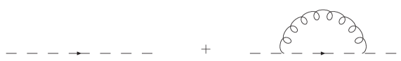
Figure 1: The one loop ghost propagator.

Explicitly, the one loop correction to the ghost self energy reads

$$\sigma(k) = g^{2}N\frac{k_{\mu}k_{\nu}}{k^{2}}\int\frac{\mathrm{d}^{2}q}{(2\pi)^{2}}\frac{1}{(k-q)^{2}}\frac{q^{2}+M^{2}}{q^{4}+M^{2}q^{2}+\lambda^{4}}\left(\delta_{\mu\nu}-\frac{q_{\mu}q_{\nu}}{q^{2}}\right)\;.$$ (23)

We recall here that the ghost self energy correction $\sigma(k)$ can be used as a kind of “order parameter” to check whether a gauge configuration lies inside or outside the Gribov horizon. Indeed, the ghost propagator is positive definite inside $\Omega$ by construction, meaning that $\sigma(k)\leq 1$. As a matter of fact, the requirement that $\sigma(k)\leq 1$ is usually called the no-pole condition, and it played a key role in Gribov’s original implementation of the restriction to the region $\Omega$ [17, 29].

Looking at the integral (23), the term $\sim\frac{1}{(q-k)^{2}}$ which could potentially lead to an infrared singularity upon integration, is partially “protected” by the external momentum $k$. One might expect that the infrared divergence will only reveal itself in the limit $k\to 0$.

Bearing this in mind, let us determine $\sigma(k)_{k^{2}\sim 0}$ by performing the $\vec{q}$-integration in (23) exactly for an arbitrary momentum $\vec{k}$. We shall invoke polar coordinates. Without loss of generality, we can put the $q_{x}$-axis along $\vec{k}$ to write

$$\sigma(k) = \frac{g^{2}N}{4\pi^{2}}\int_{0}^{\infty}q\mathrm{d}q\frac{q^{2}+M^{2}}{q^{4}+M^{2}q^{2}+\lambda^{4}}\int_{0}^{2\pi}\mathrm{d}\theta\frac{1}{k^{2}+q^{2}-2qk\cos\theta}(1-\cos^{2}\theta)\;,$$ (24)

where we made use of $\vec{k}\cdot\vec{q}=kq\cos\theta$. The Poisson-like $\theta$-integral can be easily calculated using a contour integration,

$$\int_{0}^{2\pi}\mathrm{d}\theta\frac{1-\cos^{2}\theta}{k^{2}+q^{2}-2qk\cos\theta}=\left\{\begin{array}[]{c}\frac{\pi}{q^{2}}\qquad\mbox{if\;}k^{2}\leq q^{2}\\ \frac{\pi}{k^{2}}\qquad\mbox{if\;}q^{2}\leq k^{2}\end{array}\right.\;,$$ (25)

so we obtain

$$\sigma(k) = \frac{g^{2}N}{4\pi}\left(\frac{1}{k^{2}}\int_{0}^{k}\frac{q(q^{2}+M^{2})}{q^{4}+M^{2}q^{2}+\lambda^{4}}\mathrm{d}q+\int_{k}^{\infty}\frac{q^{2}+M^{2}}{q(q^{4}+M^{2}q^{2}+\lambda^{4})}\mathrm{d}q\right)\;.$$ (26)

It appears that both integrals are well-behaved in the infrared and ultraviolet for $k>0$.

Notice that we did not invoke the gap equation (14) yet. This is possible, but neither necessary nor instructive at this point. In order to have a better understanding of the $k\to 0$ behaviour, we can calculate the integrals in (26), and extract the small momentum behaviour. Doing so, one finds

$$\left.\sigma(k)\right|_{k^{2}\sim 0}\sim-\frac{g^{2}N}{8\pi}\frac{M^{2}}{\lambda^{4}}\ln(k^{2})$$ (27)

in the case that $M^{2}\neq 0$, which is a well-defined result, in contrast with (31).

However, there is still an infrared instability in the theory due to the final $\ln(k^{2})$-factor appearing in $\sigma(k)$ for small $k$. This is our second main argument why coupling the mass operator $(\overline{\varphi}\varphi-\overline{\omega}\omega)$ to the theory causes problems:

• The quantum correction to the self energy explodes for small $k$, completely invalidating the loop expansion. This problem does not occur in $3D$ or $4D$, since there $\sigma\leq 1$. It is not difficult to imagine that the infrared $\ln(k^{2})$-singularity will spread itself through the theory, making everything ill-defined for small $k$.

• Moreover, we also encounter a problem of a more fundamental nature. The starting point of the whole construction was to always stay within the Gribov horizon $\Omega$. This can be assured by the so called no-pole condition, i.e. $\sigma(k^{2})\leq 1$ as stated in the original article by Gribov [17]. Since $M^{2}$ must be positive, we clearly see from (32) that

  $$\left.\sigma(k)\right|_{k^{2}\sim 0}\gg 1\;,$$ (28)

  hence (22) is signalling us that we have crossed the horizon.

This confirms again that $M^{2}=0$ is the only viable option, i.e. we cannot go beyond the standard Gribov-Zwanziger action if we want to avoid the appearance of destructive infrared issues, which unavoidably force the theory to leave the Gribov region.

Remark. In the previous paragraph, in order to calculate (23), we have first determined the integral in expression (23) exactly and then we have taken the limit $k^{2}\to 0$. However, one usually [17, 29] first expands the integrand for small $k^{2}$ and then performs the loop integration, as this considerably reduces the calculational effort. In the current case, this course of action unfortunately leads to incorrect results. Indeed, doing so, we would reexpress “1” as

$$1 = g^{2}N\frac{k_{\mu}k_{\nu}}{k^{2}}\int\frac{\mathrm{d}^{2}q}{(2\pi)^{2}}\frac{1}{q^{4}+M^{2}q^{2}+\lambda^{4}}\left(\delta_{\mu\nu}-\frac{k_{\mu}k_{\nu}}{k^{2}}\right)+\varsigma\frac{M^{2}}{\lambda^{2}}\;,$$ (29)

an operation which is based on the gap equation (14). Subsequently we rewrite $1-\sigma(k)$,

$$1-\sigma(k) = g^{2}N\frac{k_{\mu}k_{\nu}}{k^{2}}\int\frac{\mathrm{d}^{2}q}{(2\pi)^{2}}\frac{1}{q^{4}+\lambda^{4}}\left(1-\frac{q^{2}}{(k-q)^{2}}\right)\left(\delta_{\mu\nu}-\frac{k_{\mu}k_{\nu}}{k^{2}}\right)+\varsigma\frac{M^{2}}{\lambda^{2}}$$ (30)

$$+ g^{2}N\frac{k_{\mu}k_{\nu}}{k^{2}}\int\frac{\mathrm{d}^{2}q}{(2\pi)^{2}}\frac{1}{(k-q)^{2}}\frac{M^{2}}{q^{4}+M^{2}q^{2}+\lambda^{4}}\left(\delta_{\mu\nu}-\frac{q_{\mu}q_{\nu}}{q^{2}}\right)\;,$$

and then we expand the integrand around $k^{2}\sim 0$ to find at lowest order,

$$\left.(1-\sigma(k))\right|_{k^{2}\sim 0} = \frac{g^{2}N}{2}\int\frac{\mathrm{d}^{2}q}{(2\pi)^{2}}\frac{M^{2}}{q^{2}(q^{4}+M^{2}q^{2}+\lambda^{4})}+\varsigma\frac{M^{2}}{\lambda^{2}}+\mathcal{O}(k^{2})\;.$$ (31)

From this expression, we are led to believe that $1-\sigma(k)$, hence $\sigma(k)$, is ill-defined at small $k^{2}$, due to an infrared singularity which makes the integral in the r.h.s. of (31) to explode. However, this is not true, as in this case, the limit and the integration cannot be exchanged. The only correct way is to first calculate the integral and then take the limit as was done in the previous paragraph. Further on this section, we shall explicitly explain why expression (31) is wrong by exploring the $M^{2}=0$ case in more detail.

The case $M^{2}=0$

It is instructive to take a closer look at the usual Gribov-Zwanziger scenario. One finds for $M^{2}=0$ that

$$\left.\sigma(k)\right|_{k^{2}\sim 0}\sim\frac{g^{2}N}{4\pi}\left(\frac{\pi}{4\lambda^{2}}-\frac{k^{2}}{4\lambda^{4}}\right)\;,$$ (32)

a result which is indeed free of infrared instabilities. We also point out that ordinary (perturbative) Yang-Mills theory is recovered when $\lambda=0$. It is hence nice to observe that this again causes troubles in the infrared since the $\lambda\to 0$ limit diverges. This is just a manifestation of the fact that $2D$ gauge theories are infrared sick at the perturbative level, and need some (dynamical) regularization. Apparently, at least at the level of the ghost propagator at one loop, the Gribov mass acts a natural regulator in the infrared sector.

We should still use the gap equation in (32) to find the correct ghost propagator. The gap equation (8) for $M^{2}=0$ is readily computed as

$$\frac{2}{g^{2}N} = \int\frac{\mathrm{d}^{2}p}{(2\pi)^{2}}\frac{1}{p^{4}+\lambda^{4}}=\frac{1}{8\lambda^{2}}\;.$$ (33)

Evoking this gap equation, we find

$$1-\sigma(k) = 1-\frac{g^{2}N}{4\pi}\left(\frac{\pi}{4\lambda^{2}}-\frac{k^{2}}{4\lambda^{4}}\right)=\frac{g^{2}N}{4\pi}\frac{k^{2}}{4\lambda^{4}}=\frac{1}{\pi g^{2}N}\;.$$ (34)

Henceforth, we obtain

$$\left.{\cal G}^{ab}(k)\right|_{k^{2}\sim 0} = \left.\delta^{ab}\frac{1}{k^{2}}\frac{1}{1-\sigma(k)}\right|_{k^{2}\sim 0}=\frac{\pi g^{2}N}{k^{4}}\;.$$ (35)

We conclude that the ghost propagator is clearly enhanced and displays the typical behavior $\sim 1/k^{4}$ in the deep infrared, in accordance with the usual Gribov-Zwanziger scenario.

Remark. As we already announced earlier in this section, let us have a closer look at the $M^{2}=0$ case. In a way completely similar to the $M^{2}\neq 0$ case, we find, around $k^{2}\sim 0$,

$$\left.(1-\sigma(k))\right|_{k^{2}\sim 0} = g^{2}N\frac{k_{\mu}k_{\nu}}{k^{2}}\int\frac{\mathrm{d}^{2}q}{(2\pi)^{2}}\frac{1}{q^{4}+\lambda^{4}}\left(\frac{k^{2}}{q^{2}}-4\frac{(k\cdot q)^{2}}{q^{2}}\right)\left(\delta_{\mu\nu}-\frac{k_{\mu}k_{\nu}}{k^{2}}\right)+\mathcal{O}(k^{4})\;,$$ (36)

where we have expanded the integrand w.r.t. $q$ before integrating. Exploiting polar coordinates once more, we are now brought to

$$\left.(1-\sigma(k))\right|_{k^{2}\sim 0} = \frac{g^{2}N}{4\pi^{2}}k^{2}\int_{0}^{+\infty}\frac{q\mathrm{d}q}{q^{2}}\frac{1}{q^{4}+\lambda^{4}}\int_{0}^{2\pi}(1-4\cos^{2}\theta)(1-\cos^{2}\theta)\mathrm{d}\theta+\mathcal{O}(k^{4})\;.$$ (37)

Surprisingly, the $\theta$-integral vanishes, as it can be easily checked. In fact, one can extend this observation to all orders in $k$. To do so, we write

$$\frac{q^{2}}{(q-k)^{2}}=\frac{q^{2}}{q^{2}+k^{2}-2qk\cos\theta}=\frac{1}{1+\frac{k^{2}}{q^{2}}-2\frac{k}{q}\cos\theta}=\sum_{n=0}^{\infty}\left(\frac{k}{q}\right)^{n}{\cal U}_{n}(\cos\theta)\;,$$ (38)

where we introduced the Chebyshev polynomials of the second kind, ${\cal U}_{n}(x)$. It holds that [30]

$${\cal U}_{n}(\cos\theta) = \frac{\sin((n+1)\theta)}{\sin\theta}\;.$$ (39)

Subsequently, we can rewrite

$$1-\sigma(k) = g^{2}N\int\frac{\mathrm{d}^{2}q}{(2\pi)^{2}}\sum_{n=1}^{\infty}(1-\cos^{2}\theta){\cal U}_{n}(\cos\theta)\left(\frac{k}{q}\right)^{n}\frac{1}{q^{4}+\lambda^{4}}\;,$$ (40)

where use has been made of ${\cal U}_{0}(x)=1$. Assuming that the integral and the infinite sum can be interchanged, we are led to

$$1-\sigma(k) = \frac{g^{2}N}{4\pi^{2}}\sum_{n=1}^{\infty}k^{n}\int_{0}^{+\infty}\frac{\mathrm{d}q}{q^{n-1}}\frac{1}{q^{4}+\lambda^{4}}\int_{0}^{2\pi}(1-\cos^{2}\theta){\cal U}_{n}(\cos\theta)\mathrm{d}\theta\;.$$ (41)

Since $n\geq 1$ and making use of (39), for the $\theta$-integration we find

$$\int_{0}^{2\pi}(1-\cos^{2}\theta){\cal U}_{n}(\cos\theta)\mathrm{d}\theta = \int_{0}^{2\pi}\sin\theta\sin((n+1)\theta)\mathrm{d}\theta$$ (42)

$$= \int_{0}^{2\pi}\frac{\cos(n\theta)-\cos((n+2)\theta)}{2}\mathrm{d}\theta=0\;.$$

However, this does not make the integral in (41) well defined, as the remaining $q$-integral is infrared singular for any occurring value of $n$! In fact, exactly these infrared divergences forbid the interchange of integral and of the infinite sum. This is a nice example of the fact that the integral of a infinite sum can be well defined, whereas the (sum of the) individual integrals are not.

When we first integrate exactly for any $k$ and then expand in powers of $k^{2}$, we do recover the meaningful result (34) at $k^{2}\sim 0$.

4 The gluon propagator and positivity violation

Before turning to the conclusion, we would like to recall that another typical feature of the Gribov-Zwanziger scenario is that the gluon propagator vanishes at zero momentum. More precisely, ${\cal D}(0)=0$. This implies a maximal violation of positivity, see e.g. [16], thereby signalling that the gluon is an unphysical degree of freedom and hence “confined”.

In $3D$ and $4D$, we have shown that the effects originating from the coupling of the operator $\overline{\varphi}\varphi-\overline{\omega}\omega$ to the theory gives a finite nonzero value to ${\cal D}(0)$, in accordance with the lattice data [16, 24]. Notice, however, that there is still a clear violation of positivity notwithstanding that ${\cal D}(0)\neq 0$. Our results were in qualitative agreement with the available lattice data [16, 24].

As we have argued already, we must discard $\overline{\varphi}\varphi-\overline{\omega}\omega$ in $2D$. Consequently, ${\cal D}(0)$ still vanishes in $2D$ at tree level due to the Gribov mass, as it is immediately verified from

$${\cal D}(p^{2})=\frac{p^{2}}{p^{4}+\lambda^{4}}\;.$$ (43)

In principle, one could explicitly check whether this persists beyond tree level order. However, this leads to quite complicated loop calculations, as can be appreciated from the $4D$ or $3D$ counterpart done in [16, 24], and therefore we shall not pursue this here.

5 Conclusion

In this letter, we have discussed why it is not possible to “refine” the Gribov-Zwanziger action in $2D$, in contrast with the $3D$ or $4D$ case. In the latter case, we have shown in recent work [15, 16, 24] that the inclusion of dynamical effects related to a novel mass operator, constructed with the additional field present in the Gribov-Zwanziger action, has a profound influence on the infrared behaviour of the theory, and considerably changes the usual Gribov-Zwanziger predictions. The main conclusion is that the ghost propagator is not infrared enhanced but retains its $\frac{1}{q^{2}}$ singularity in the deep infrared, while the gluon propagator becomes finite and nonvanishing at zero momentum. The usual Gribov-Zwanziger scenario predicts a $1/k^{4}$ singularity for the ghost propagator, and a vanishing gluon propagator at zero momentum, ${\cal D}(0)=0$. Surprisingly, lattice data at large volumes are in compliance with the refined analytical results presented in [15, 16, 24]. Since the lattice data in $2D$ still predicts an infrared enhanced ghost and vanishing ${\cal D}(0)$ [12, 13, 14], we were motivated to discuss how this would fit into our refined Gribov-Zwanziger scenario [15, 16]. We have shown that it is not possible to couple the particular operator, $\overline{\varphi}\varphi-\overline{\omega}\omega$, to the action in $2D$, as it triggers serious infrared instabilities, which are peculiar to the $2D$ case. Thence, the usual Gribov-Zwanziger scenario is so to say “protected” in $2D$. In fact, we have proven that the emerging infrared singularities make it impossible to stay within the Gribov region $\Omega$ when $M^{2}\neq 0$. As a nice byproduct of this work, we have seen that the Gribov mass can act as a natural infrared regulator, stabilizing the otherwise ill-defined perturbative expansion.

References

- [1] G. ’t Hooft, Nucl. Phys. B 75 (1974) 461.
- [2] A. Bassetto, Nucl. Phys. Proc. Suppl. 88 (2000) 184.
- [3] Y. Frishman, C. T. Sachrajda, H. D. I. Abarbanel and R. Blankenbecler, Phys. Rev. D 15 (1977) 2275.
- [4] N. K. Pak and H. C. Tze, Phys. Rev. D 14 (1976) 3472.
- [5] T. T. Wu, Phys. Lett. B 71 (1977) 142.
- [6] R. Alkofer, C. S. Fischer, F. J. Llanes-Estrada and K. Schwenzer, arXiv:0804.3042 [hep-ph].
- [7] T. Kugo and I. Ojima, Prog. Theor. Phys. Suppl. 66 (1979) 1.
- [8] T. Kugo, arXiv:hep-th/9511033.
- [9] J. Braun, H. Gies and J. M. Pawlowski, arXiv:0708.2413 [hep-th].
- [10] A. Cucchieri and T. Mendes, PoS LATTICE (2007) 297.
- [11] I. L. Bogolubsky, E. M. Ilgenfritz, M. Muller-Preussker and A. Sternbeck, PoS LATTICE (2007) 290.
- [12] A. Cucchieri and T. Mendes, Phys. Rev. Lett. 100 (2008) 241601.
- [13] A. Cucchieri and T. Mendes, arXiv:0804.2371 [hep-lat].
- [14] A. Maas, Phys. Rev. D 75 (2007) 116004.
- [15] D. Dudal, S. P. Sorella, N. Vandersickel and H. Verschelde, Phys. Rev. D 77 (2008) 071501.
- [16] D. Dudal, J. Gracey, S. P. Sorella, N. Vandersickel and H. Verschelde, Phys. Rev. D, to appear, arXiv:0806.4348 [hep-th].
- [17] V. N. Gribov, Nucl. Phys. B 139 (1978) 1.
- [18] D. Zwanziger, Nucl. Phys. B 323 (1989) 513.
- [19] D. Zwanziger, Nucl. Phys. B 399 (1993) 477.
- [20] Semenov-Tyan-Shanskii and V.A. Franke, Zapiski Nauchnykh Seminarov Leningradskogo Otdeleniya Matematicheskogo Instituta im. V.A. Steklov AN SSSR}, Vol. 120 (1982) 159. English translation: New York: Plenum Press 1986.
- [21] G. Dell’Antonio and D. Zwanziger, Commun. Math. Phys. 138 (1991) 291.
- [22] G. Dell’Antonio and D. Zwanziger, Proceedings of the NATO Advanced Research Workshop on Probabilistic Methods in Quantum Field Theory and Quantum Gravity, Cargèse, August 21-27, 1989, Damgaard and Hueffel (eds.), p.107, New York: Plenum Press.
- [23] P. van Baal, Nucl. Phys. B 369 (1992) 259.
- [24] D. Dudal, J. A. Gracey, S. P. Sorella, N. Vandersickel and H. Verschelde, arXiv:0808.0893 [hep-th].
- [25] D. Zwanziger, Phys. Rev. D 65 (2002) 094039.
- [26] A. Maas, J. Wambach, B. Gruter and R. Alkofer, Eur. Phys. J. C 37 (2004) 335.
- [27] M. Q. Huber, R. Alkofer, C. S. Fischer and K. Schwenzer, Phys. Lett. B 659 (2008) 434.
- [28] O. Piguet and S. P. Sorella, Lect. Notes Phys. M28 (1995) 1.
- [29] R. F. Sobreiro and S. P. Sorella, arXiv:hep-th/0504095.
- [30] http://mathworld.wolfram.com.