Jamming in Fixed-Rate Wireless Systems with Power Constraints - Part II: Parallel Slow Fading Channels

Abstract

This is the second part of a two-part paper that studies the problem of jamming in a fixed-rate transmission system with fading. In the first part, we studied the scenario with a fast fading channel, and found Nash equilibria of mixed strategies for short term power constraints, and for average power constraints with and without channel state information (CSI) feedback. We also solved the equally important maximin and minimax problems with pure strategies. Whenever we dealt with average power constraints, we decomposed the problem into two levels of power control, which we solved individually. In this second part of the paper, we study the scenario with a parallel, slow fading channel, which usually models multi-carrier transmissions, such as OFDM. Although the framework is similar as the one in Part I [1], dealing with the slow fading requires more intricate techniques. Unlike in the fast fading scenario, where the frames supporting the transmission of the codewords were equivalent and completely characterized by the channel statistics, in our present scenario the frames are unique, and characterized by a specific set of channel realizations. This leads to more involved inter-frame power allocation strategies, and in some cases even to the need for a third level of power control. We also show that for parallel slow fading channels, the CSI feedback helps in the battle against jamming, as evidenced by the significant degradation to system performance when CSI is not sent back. We expect this degradation to decrease as the number of parallel channels $M$ increases, until it becomes marginal for $M\to\infty$ (which can be considered as the case in Part I).

Keywords: Slow fading channels, outage probability, jamming, zero-sum game, fixed rate, power control.

I Introduction

The concept of jamming plays an extremely important role in ensuring the quality and security of wireless communications, especially at this moment when wireless networks are quickly becoming ubiquitous. Although the recent literature covers a wide variety of jamming problems [2, 3, 4, 5, 6, 7, 8], the investigation of optimal jamming and anti-jamming strategies for the parallel slow-fading channel is missing.

The parallel slow-fading channel is a widely used model for OFDM transmission [9]. Since the usual definition of capacity does not provide a positive performance indicator for this model, a more adequate performance measure is the probability of outage [9], defined as the probability that the instantaneous mutual information characterizing the parallel channel, under a given channel realization, is below a fixed transmission rate $R$. Under the optimal diversity-multiplexing tradeoff, the parallel slow-fading channel with $M$ subchannels is known [9] to yield an $M$-fold diversity gain over the scalar single antenna channel. However the diversity-multiplexing tradeoff only gives an approximative analytical evaluation of the probability of outage for a given rate $R$ and a signal-to-noise ratio (SNR), and this approximation is usually accurate only in the high SNR region. Thus, for evaluating a system which functions at a moderate SNR, the exact probability-of-outage vs. transmission-rate curve is often computed numerically. Moreover, the high SNR assumption is clearly not adequate for studying a practical uncorrelated jamming situation, where the jammer’s power should be considered at least comparable to the legitimate transmitter’s.

Therefore, we aim at deriving the exact probability of outage achievable in the presence of a jammer, over our parallel slow fading channel, for a fixed transmission rate $R$. Our channel model is depicted in Figure 1. The span of a codeword is denoted by “frame”. To model our parallel slow fading channel, each frame is divided into $M$ “blocks” (corresponding to the $M$ subchannels), each of which consists of $N$ channel uses, like in Figure 2.

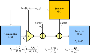
Figure 1: Channel model

The channel fading is slow, such that the corresponding channel coefficients remain constant over each block and vary independently across different blocks. The channel coefficients are complex numbers, and their squared absolute values are denoted as $h_{m}$. The vector $\mathbf{h}=[h_{0},h_{1},\ldots,h_{M-1}]$ of channel coefficients over a whole frame is assumed to be perfectly known to the receiver, and can be made available by feedback (if the receiver wishes) to the transmitter (Tx), and jammer (Jx) before the transmission begins. It was shown in [10] that the feedback of channel state information (CSI) (i.e. the $M$ coefficients of a frame) brings moderate benefits for the parallel slow-fading channel without jamming. Thus, by employing optimal power control strategies, the transmitter can lower the probability of outage for fixed transmission rate and SNR. In this paper, we study both the scenarios when the CSI is fed back by the legitimate receiver – and hence all $M$ channel coefficients characterizing a frame are available to both transmitter and jammer in a non-causal fashion (it is only natural to assume that if the transmitter has full CSI, the jammer can get the same information by eavesdropping) – and the scenario when no feedback takes place and thus the CSI is only available to the receiver.

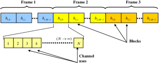
Figure 2: Frames, blocks and channel uses

In addition to fading, the transmission is affected by additive white complex Gaussian noise (AWGN), and by a jammer. The jammer has no knowledge about the transmitter’s output, or even the codebook that the transmitter is using, and hence it deploys its most harmful strategy: it transmits white complex Gaussian noise [11] (AWGJ in Figure 1).

The transmitter (Tx) uses a complex Gaussian codebook. Over a given frame, it allocates power $P_{m}$ to block $m$, $0\leq m\leq M-1$, while the jammer (Jx) invests power $J_{m}$ in jamming the same block with noise. As assumed in [10], the number of channel uses per block is large $N\to\infty$ in order to average out the impact of the Gaussian noise. Under these assumptions, the instantaneous mutual information characterizing a subchannel $m$ is given by $I(h_{m},P_{m},J_{m})=\log(1+\frac{h_{m}P_{m}}{\sigma_{N}^{2}+J_{m}})$, where $\sigma_{N}^{2}$ is the variance of the ambient AWGN. The following denotations will be repeatedly used in the sequel:

• Power allocated by the transmitter over a frame:
  $P_{M}=\frac{1}{M}\sum_{m=0}^{M-1}P_{m}$;

• Power allocated by the jammer over a frame:
  $J_{M}=\frac{1}{M}\sum_{m=0}^{M-1}J_{m}$;

• Instantaneous mutual information between the transmitter and the receiver over a frame:
  $I_{M}=\frac{1}{M}\sum_{m=0}^{M-1}I(h_{m},P_{m},J_{m})$.

Note that $P_{M}$ is a function of the channel realization $\mathbf{h}$, so we often write $P_{M}(\mathbf{h})$ when this relation needs to be explicitly emphasized. $P_{M}(\mathbf{h})$ can also be interpreted as the function giving the power distribution across different frames. We also use $P_{M}(h)$ and $J_{M}(h)$ to denote inter-frame power allocation for the case $M=1$, since in this case a frame only contains one block. Like in [1], throughout this paper we shall also use the notation $c=\exp(MR)$ for simplicity.

As depicted in Figure 1, our channel model is similar to that of [2]. The difference, however, is that we investigate the jamming problem in slow-fading channels and hence the probability of outage, defined as the probability that the instantaneous mutual information $I_{M}$ of the channel is lower than the fixed transmission rate $R$ [10] is considered as an objective function $P_{out}=Pr(I_{M}<R)$ (while [2] assumes fast fading and uses the ergodic capacity as objective). Our problem is still formulated as a two-player, zero-sum game. The transmitter wants to achieve reliable communication and hence minimize the outage probability, while the jammer wants to induce outage and maximize the outage probability. Strategies consist of varying transmission powers based on the CSI (i.e. the perfect knowledge of $\mathbf{h}$) if available, or solely on the channel’s statistics if CSI is not available. The properties of our different objective function make our new jamming and anti-jamming problem much more challenging to solve.

It is easy to find similarities to the fixed rate system with fast fading which was studied in the first part of this paper [1]. In fact, the fast fading scenario of [1] can be obtained as a particular case of the current setup, by allowing a large number of blocks per frame $M\to\infty$ (corresponding to an infinite number of subchannels). In doing so, the different frames are no longer characterized by their respective channel realizations, but instead they become long enough to display the statistical properties of the channel coefficient and thus become equivalent. This is why our present parallel slow fading scenario is more involved than the fast fading model of Part I of this paper [1], especially when it comes to resolving the optimal power allocation between different frames. Sometimes this additional complexity leads to an additional level of power control, as we shall see in Section IV.

Our contributions are summarized below:

• We first investigate the case where the receiver feeds back the channel state information (CSI) which becomes available to both transmitter and jammer. For the short-term power constraints case we show the existence of and find a Nash equilibrium of pure strategies. Note that for a two-person, zero-sum game, all Nash equilibria have the same value [12]. Since an equilibrium of pure strategies is also an equilibrium of mixed strategies, our Nash equilibrium of pure strategies provides the complete solution of the game.

• For the case with long-term power constraints we find the maximin and minimax solutions of pure strategies, and show they do not coincide (hence the non-existence of a Nash equilibrium of pure strategies). Traditional methods of optimization, such as the KKT conditions, cannot be applied to solve for these solutions completely. Therefore we provide a new, more intuitive approach based on the special duality property discussed in Appendix II-D of the first part of this paper [1]. As argued in [1], Nash equilibria of mixed strategies may not always be the best solutions to jamming problems. A smart jammer could eavesdrop the channel and detect both the legitimate transmitter’s presence and its power level. Therefore, we believe that the maximin and minimax problem formulations with pure strategies are of great importance in understanding and resolving the practical jamming situations (in the worst case, they provide upper and lower bounds on the system’s performance).

• The optimal pure strategies of allocating power between frames, for the maximin and minimax formulations, are found as the solutions of two simple numerical algorithms. These algorithms function according to two different techniques which we explain in the sequel and we dub as “the vase water filling problems”.

• Mixed strategies are discussed next. We show that for completely characterizing this scenario we need three different levels of power control. We then particularize and obtain numerical results for the special simple case with only one block per frame ($M=1$).

• Finally, we compare our results to the case when the channel state information is only available to the receiver. We derive a Nash equilibrium for $M=1$, and show that unlike in the fast fading scenario (where CSI feedback brings negligible improvements), under our current parallel slow fading channel model, perfect knowledge about the CSI at all parties can substantially improve performance.

The paper is organized as follows. Section II deals with the short term power constrained problem when full CSI is available to all parties. Section III studies the scenario with long term power constraints and pure strategies under the same assumption of available CSI. Mixed strategies are discussed in Section IV. For comparison purposes, Section V presents results for the case with no CSI feedback. Finally, conclusions are drawn in Section VI.

II CSI Available to All Parties. Jamming Game with Short-Term Power Constraints

The game with short-term power constraints is the less complex of the two games we discuss in the sequel. In this game, the transmitter’s goal is to:

$$\left\{\begin{array}[]{cc}\textrm{Minimize}&\mbox{Pr}(I_{M}(\mathbf{h},P(h),J(h))<R)\\ \textrm{Subject to}&P_{M}(\mathbf{h})\leq\mathcal{P},\textrm{with prob. 1}\end{array}\right.$$ (3)

while the jammer’s goal is to:

$$\left\{\begin{array}[]{cc}\textrm{Maximize}&\mbox{Pr}(I_{M}(\mathbf{h},P(h),J(h))<R)\\ \textrm{Subject to}&J_{M}(\mathbf{h})\leq\mathcal{J},\textrm{with prob. 1}.\end{array}\right.$$ (6)

We shall prove that this game is closely related to a different two player, zero-sum game, which has the mutual information between Tx and Rx as a cost/reward function:

$$\textrm{Tx}\left\{\begin{array}[]{cc}\textrm{Maximize}&I_{M}(\mathbf{h},P(h),J(h))\\ \textrm{Subject to}&P_{M}(\mathbf{h})\leq\mathcal{P},\end{array}\right.$$ (9)

$$\textrm{Jx}\left\{\begin{array}[]{cc}\textrm{Minimize}&I_{M}(\mathbf{h},P(h),J(h))\\ \textrm{Subject to}&J_{M}(\mathbf{h})\leq\mathcal{J}.\end{array}\right.$$ (12)

This latter game is characterized by the following proposition:

Proposition 1

The game of (9) and (12) has a Nash equilibrium point given by the following strategies:

$$P^{*}(h_{m})=\left\{\begin{array}[]{ccc}(\frac{1}{\eta}-\frac{\sigma_{N}^{2}}{h_{m}})^{+}&\textrm{if}&h_{m}<\frac{\sigma_{N}^{2}\eta}{1-\sigma_{N}^{2}\nu}\\ \frac{h_{m}}{\eta(h_{m}+\frac{\eta}{\nu})}&\textrm{if}&h_{m}\geq\frac{\sigma_{N}^{2}\eta}{1-\sigma_{N}^{2}\nu}\end{array}\right.$$ (15)

$$J^{*}(h_{m})=\left\{\begin{array}[]{ccc}0&\textrm{if}&h_{m}<\frac{\sigma_{N}^{2}\eta}{1-\sigma_{N}^{2}\nu}\\ \frac{h_{m}}{\nu(h_{m}+\frac{\eta}{\nu})}-\sigma_{N}^{2}&\textrm{if}&h_{m}\geq\frac{\sigma_{N}^{2}\eta}{1-\sigma_{N}^{2}\nu}\end{array}\right.$$ (18)

where $\eta$ and $\nu$ are constants that can be determined from the power constraints.

Proof:

The proof is a straightforward adaptation of Section IV.B in [2], and is outlined in Appendix A. ∎

The connection between the two games above is made clear in the following theorem, the proof of which follows in the footsteps of [10] and is given in Appendix A.

Theorem 1

Let $P^{*}(h)$ and $J^{*}(h)$ denote the Nash equilibrium solutions of the game described by (9) and (12). Then the original game of (3), (6) has a Nash equilibrium point, which is given by the following pair of strategies:

$$\widehat{P}(h_{m})=\left\{\begin{array}[]{ccc}P^{*}(h_{m})&\textrm{if}&\mathbf{h}\in\mathcal{U}(R,\mathcal{P},\mathcal{J})\\ P_{a}(h_{m})&\textrm{if}&\mathbf{h}\notin\mathcal{U}(R,\mathcal{P},\mathcal{J})\end{array}\right.$$ (21)

$$\widehat{J}(h_{m})=\left\{\begin{array}[]{ccc}J_{a}(h_{m})&\textrm{if}&\mathbf{h}\in\mathcal{U}(R,\mathcal{P},\mathcal{J})\\ J^{*}(h_{m})&\textrm{if}&\mathbf{h}\notin\mathcal{U}(R,\mathcal{P},\mathcal{J})\end{array}\right.$$ (24)

where $\mathcal{U}(R,\mathcal{P},\mathcal{J})=\{\mathbf{h}\in\mathbb{R}_{+}^{M}:I_{M}(\mathbf{h},P^{*}(h),J^{*}(h))\geq R\}$, and where $P_{a}(h)$ and $J_{a}(h)$ are some arbitrary power allocations satisfying the power constraints respectively.

III CSI Available to All Parties. Jamming Game with Long-Term Power Constraints: Pure Strategies

The long-term power constrained jamming game can be formulated as:

$$\textrm{Tx}\left\{\begin{array}[]{cc}\textrm{Minimize}&\mbox{Pr}(I_{M}(\mathbf{h},\{P_{m}\},\{J_{m}\})<R)\\ \textrm{Subject to}&E[P_{M}(\mathbf{h})]\leq\mathcal{P}\end{array}\right.$$ (27)

$$\textrm{Jx}\left\{\begin{array}[]{cc}\textrm{Maximize}&\mbox{Pr}(I_{M}(\mathbf{h},\{P_{m}\},\{J_{m}\})<R)\\ \textrm{Subject to}&E[J_{M}(\mathbf{h})]\leq\mathcal{J}\end{array}\right.$$ (30)

where the expectation is taken with respect to the vector of channel coefficients $\mathbf{h}=(h_{0},h_{1},\ldots,h_{M-1})\in\mathbb{R}_{+}^{M}$, and $\mathcal{P}$ and $\mathcal{J}$ are the upper-bounds on average transmission power of the source and jammer, respectively.

Contrary to the previous short-term power constraints scenario, if long-term power constraints are used it is possible to have $P_{M}(\mathbf{h})>\mathcal{P}$ for a particular channel realization $\mathbf{h}$, as long as the average of $P_{M}(\mathbf{h})$ over all possible channel realizations is less than $\mathcal{P}$.

Let $\mathfrak{m}$ denote the probability measure introduced by the probability density function (p.d.f.) of $\mathbf{h}$, i.e., for a set $\mathscr{A}\subseteq\mathbb{R}_{+}^{M}$, we have $\mathfrak{m}(\mathscr{A})=\int_{\mathscr{A}}f(\mathbf{h})d\mathbf{h}$. Integrating with respect to this measure is equivalent to computing an average with respect to the p.d.f. given by $f(\mathbf{h})$, i.e., $d\mathfrak{m}(\mathbf{h})=f(\mathbf{h})d\mathbf{h}$.

Both transmitter and jammer have to plan in terms of power allocation, considering both the instantaneous realization and the probability distribution of the channel coefficient vector, as well as their opponent’s strategy.

If the number of blocks $M$ in each frame is larger than $1$, the game between transmitter and jammer has two levels. The first (coarser) level is about power allocation between frames, and has the probability of outage as a cost/reward function. This is the only level that shows up in the case of $M=1$. The second (finer) level is that of power allocation between the blocks within a frame.

An important comment similar to that in [1] needs to be made. We should point out that decomposing the problem into several (two or three) levels of power control, each of which is solved separately, does not restrict the generality of our solution. In proving our main results we take a contradictory approach. That is, instead of directly deriving each optimal strategy, we assume an optimal solution has already been reached and show it has to satisfy a set of properties. We do this by first assuming that the properties are not satisfied, and then showing that under this assumption at least one of the players can improve its strategy (and hence the original solution cannot be optimal). The properties are selected such that they are not only necessary, but also sufficient for the completely characterizing the optimal solution (i.e. there exists a unique pair of strategies that satisfy these properties).

III-A Power Allocation between the blocks in a Frame

In this subsection we only deal with the second (intra-frame) level of power allocation for the maximin and minimax problems. The first (inter-frame) level will be investigated in detail in the following two subsections.

The probability of outage is determined by the $\mathfrak{m}$-measure of the set over which the transmitter is not present or the jammer is successful in inducing outage. This set is established in the first level of power control. Note that the first level power allocation strategies cannot be derived before the second level strategies are available.

In the maximin case (when the jammer plays first), assume that the jammer has already allocated some power $J_{M}$ to a given frame. Naturally, the transmitter knows $J_{M}$ (the maximin problem assumes that the transmitter is fully aware of the jammer’s strategy). Depending on the channel realization, the value of $J_{M}$, and its own power constraints, the transmitter decides whether it wants to achieve reliable communication over that frame. If it decides to transmit, it needs to spend as little power as possible (the transmitter will be able to use the saved power for achieving reliable communication over another set of positive $\mathfrak{m}$-measure, and thus to decrease the probability of outage). Therefore, the transmitter’s objective is to minimize the power $P_{M}$ spent for achieving reliable communication. The transmitter will adopt this strategy whether the jammer is present over the frame, or not. The jammer’s objective is then to allocate $J_{M}$ between the blocks such that the required $P_{M}$ is maximized.

In the minimax scenario (when transmitter plays first) the jammer’s objective is to minimize the power $J_{M}$ used for jamming the transmission over a given frame. The jammer will only transmit if the transmitter is present with some $P_{M}$. The transmitter’s objective is to distribute $P_{M}$ between blocks such that the power required for jamming is maximized.

The two problems can be formulated as:

Problem 1 (for the maximin solution - jammer plays first)

$$\max_{\{J_{m}\geq 0\}}\Big{[}\min_{\{P_{m}\geq 0\}}P_{M}=\frac{1}{M}\sum_{m=0}^{M-1}P_{m},$$

$$~{}\textrm{s.t.}~{}I_{M}(\{P_{m}\},\{J_{m}\})\geq R\Big{]}\textrm{s.t.}\frac{1}{M}\sum_{m=0}^{M-1}J_{m}\leq J_{M};$$ (31)

Problem 2 (for the minimax solution - transmitter plays first)

$$\max_{\{P_{m}\geq 0\}}\Big{[}\min_{\{J_{m}\geq 0\}}J_{M}=\frac{1}{M}\sum_{m=0}^{M-1}J_{m},$$

$$~{}\textrm{s.t.}~{}I_{M}(\{P_{m}\},\{J_{m}\})\leq R\Big{]}\textrm{s.t.}\frac{1}{M}\sum_{m=0}^{M-1}P_{m}\leq P_{M}.$$ (32)

These problems can be solved by methods very similar to those presented in the first part of this paper [1]. For the brevity of this presentation, we shall only point out the main results, and defer all proofs to the Appendix B. The following propositions fully characterize the solutions.

Proposition 2

The optimal solution of either of the two problems above satisfies both constraints with equality.

Proposition 3

(I) Take the game given by (9) and (12) and set the constraints to $P_{M}(\mathbf{h})\leq P_{M,1}$ and $J_{M}(\mathbf{h})\leq J_{M,1}$. Denote the resulting value of the objective by $I_{M}(\mathbf{h},P(h),J(h))=R_{1}$. Then solving Problem 1 above with the constraints $\frac{1}{M}\sum_{m=0}^{M-1}J_{m}\leq J_{M,1}$ and $I_{M}(\{P_{m}\},\{J_{m}\})\geq R_{1}$ yields the objective $P_{M}=P_{M,1}$. Moreover, any pair of power allocations across blocks that makes an optimal solution of the game in (9) and (12) is also an optimal solution of Problem 1, and conversely.

(II)Take the game given by (9) and (12) and set the constraints to $P_{M}(\mathbf{h})\leq P_{M,1}$ and $J_{M}(\mathbf{h})\leq J_{M,1}$. Denote the resulting value of the objective by $I_{M}(\mathbf{h},P(h),J(h))=R_{1}$. Then solving Problem 2 above with the constraints $\frac{1}{M}\sum_{m=0}^{M-1}P_{m}\leq P_{M,1}$ and $I_{M}(\{P_{m}\},\{J_{m}\})\leq R_{1}$ yields the objective $J_{M}=J_{M,1}$. Moreover, any pair of power allocations across blocks that makes an optimal solution of the game in (9) and (12) is also an optimal solution of Problem 2, and conversely.

(III) If $J_{M,1}$ is the value used for the second constraint in Problem 1 above, and $P_{M,1}$ is the resulting value of the cost/reward function, then solving Problem 2 with $P_{M}=P_{M,1}$ yields the cost/reward function $J_{M}=J_{M,1}$. Moreover, any pair of power allocations across blocks that makes an optimal solution of Problem 1, should also make an optimal solution of Problem 2, and conversely.

Proposition 4

The optimal solutions of Problem 1 and Problem 2 above are unique.

Proposition 5

(I) Under the optimal maximin second level power control strategies (Problem 1), the “required” transmitter power $P_{M}$ over a frame is a strictly increasing, continuous, concave and unbounded function of the power $J_{M}$ that the jammer invests in that frame.

(II) Under the optimal minimax second level power control strategies (Problem 2), the “required” jamming power $J_{M}$ over a frame is a strictly increasing, continuous, convex and unbounded function of the power $P_{M}$ that the transmitter invests in that frame.

Although under the same transmitter/jammer frame power constraints $P_{M}$ and $J_{M}$ the second level optimal power allocation strategies for the maximin and minimax problems coincide, this result should not be associated with the notion of Nash equilibrium, since the two problems solved above do not form a zero-sum game, while for the game of (27) and (30), first level power control strategies are yet to be investigated.

As in [1], we shall henceforth denote the function that gives the “required” transmitter power $P_{M}$ over a frame where the jammer invests power $J_{M}$ by $\mathscr{P}_{M}(J_{M},\mathbf{h})$ and its “inverse”, i.e. the function that gives the “required” jamming power over a frame where the transmitter invests $P_{M}$ by $\mathscr{J}_{M}(P_{M},\mathbf{h})$. Note that unlike in [1], these functions are now also dependent on the channel realization $\mathbf{h}$. A particular channel realization can be characterized in terms of the second level power allocation technique. For instance, considering the maximin problem, we can map each channel vector $\mathbf{h}$ to a unique curve $\mathscr{P}_{M}(J_{M})$ in the plane. That is, for fixed $\mathbf{h}$, we increase the jamming power allocated to the frame from $0$ to $\infty$, and compute the transmitter power $\mathscr{P}_{M}(J_{M},\mathbf{h})$ required for achieving reliable communication. We have already mentioned that, for any fixed $\mathbf{h}$, $\mathscr{P}_{M}(J_{M})$ is a strictly increasing, continuous, concave and unbounded function.

Next we take a closer look at the $\mathscr{P}_{M}(J_{M},\mathbf{h})$ curves. By inspecting the proofs of Propositions 2 - 5, we notice that $j$ denotes the index of the first block on which the jammer allocates nonzero power, while $p$ is the index of the first block on which the transmitter allocates nonzero power (the blocks are indexed in increasing order of their squared channel coefficients $h_{m}$, and both transmitter and jammer allocate more power to blocks with larger values of $h_{m}$). Note also that $p\leq j$. If for a given $\mathbf{h}$ we have $p=j$ over an interval of $J_{M}$, then the $\mathscr{P}_{M}(J_{M})$ curve is linear over that interval. However, if $p<j$, the curve is strictly concave.

We can think of the $\mathscr{P}_{M}(J_{M})$ curve that characterizes a given channel realization $\mathbf{h}$ as being “built” in the following manner. We increase the jamming power allocated to the corresponding frame, starting from $J_{M}=0$. We already know that without the jammer’s presence the transmitter transmits over the “best” blocks , i.e. the ones having the largest channel coefficients. Even as the jammer starts interfering, its optimal strategy is such that the blocks with the largest coefficients remain the most attractive for the transmitter. However, they do become worse than before. Hence, if without the presence of the jammer the transmitter would normally ignore some of the blocks, as the jammer’s power increases, those blocks may slowly become more attractive. At some point, the transmitter will choose to increase the number of blocks over which it allocates non-zero power (i.e. decrease $p$). Similarly, as the jammer’s power $J_{M}$ increases, the jammer moves from the best block to the best two blocks, and so on (i.e. the jammer decreases $j$).

The transmitter’s and the jammer’s transitions do not have to be simultaneous. Recall that the relationship between the values of $p$ and $j$ decide whether the $\mathscr{P}_{M}(J_{M})$ curve is linear or strictly concave over an interval of $J_{M}$. Therefore, we expect the $\mathscr{P}_{M}(J_{M})$ curves to look like a concatenation of linear and strictly concave segments, as in Figure 3. As $J_{M}$ increases, the transmitter decreases the value of $p$ whenever the slope of the $\mathscr{P}_{M}(J_{M})$ curve can be decreased by this move and similarly, the jammer decreases the value of $j$ whenever the slope can be increased. In other words, as $J_{M}$ increases, the transitions from linear portions to nonlinear portions are caused by the transmitter, while the transitions from nonlinear to linear ones are caused by the jammer.

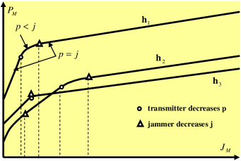
Figure 3: Typical $P_{M}(J_{M})$ curves, for different channel realizations

In the remainder of this subsection we provide the simplest example of optimal power allocation between the blocks of a frame. Namely, we look at the case when $M=2$ – only two blocks per frame.

Particular case: $M=2$

The case of $M=2$ is the simplest and most intuitive illustration of the second-level power control strategy. Since we have already discussed the nice dual property between the second level minimax and maximin strategies, the following considerations refer to the maximin scenario only. The jamming power $J_{M}$ has to be allocated between the two blocks in a way that maximizes the transmitter’s expense, should it decide to achieve reliable communication over the frame. The jammer and the transmitter can each transmit over either one or both blocks. All possible situations are considered next.

Let the two channel coefficients be $h_{0}\leq h_{1}$, and denote the transmitter’s and jammer’s powers allocated to the blocks by $P_{0},P_{1}$ and $J_{0},J_{1}$ respectively. Also denote $x_{i}=J_{i}+\sigma_{N}^{2}$, for $i\in\{0,1\}$, and $c=\exp(2R)$. If we take a closer look at the solutions (15) and (18) of the game in (9) and (12), and if we recall that the solutions of either of our maximin and minimax second layer power allocation strategies have a similar form (up to the constants $\eta$ and $\nu$), it is easy to observe that $x_{0}\leq x_{1}$ and $\frac{x_{0}}{h_{0}}\geq\frac{x_{1}}{h_{1}}$. This fact is also noted in Appendix B-C, where the solution of Problem 1 is given again, with the new notation $\lambda=1/\eta$ and $\mu=\nu/\eta$. Throughout the rest of this subsection we shall refer to the notation in Appendix B-C and the solution in (128) and (131).

If the transmitter is active over both blocks, then the constraint $I_{M}=R$ yields

$$\left(1+\frac{h_{0}}{x_{0}}P_{0}\right)\left(1+\frac{h_{1}}{x_{1}}P_{1}\right)=c,$$ (33)

and with (132) in Appendix B-C we obtain $\lambda=\sqrt{c\frac{x_{0}}{h_{0}}\frac{x_{1}}{h_{1}}}$.

Suppose that the jammer is only present on one block of the frame, then that is the block with coefficient $h_{1}$. This implies $x_{0}=\sigma_{N}^{2}$, and $x_{1}=(2J_{M}+\sigma_{N}^{2})$. Under these assumptions, the transmitter will only transmit on the first block, (that is $P_{0}=2P_{M}$ and $P_{1}=0$) if and only if

$$\lambda=\sqrt{c\frac{x_{0}}{h_{0}}\frac{x_{1}}{h_{1}}}<\frac{x_{0}}{h_{0}},$$ (34)

which translates to $c\frac{(2J_{M}+\sigma_{N}^{2})}{h_{1}}<\frac{\sigma_{N}^{2}}{h_{0}}$.

Otherwise, the transmitter is present over both blocks, performing water-pouring as in (132), with

$$\lambda=\sqrt{c\frac{(2J_{M}+\sigma_{N}^{2})\sigma_{N}^{2}}{h_{0}h_{1}}}.$$ (35)

Note that the transmitter cannot be present only on the second block.

If the jammer decides to allocate non-zero power over both blocks, its optimal strategy is such that $x_{0}/h_{0}\geq x_{1}/h_{1}$. If we also have $x_{0}/h_{0}\leq c(x_{1}/h_{1})$ (corresponding to $\lambda\geq x_{0}/h_{0}$), then the transmitter is present over both blocks. In this case, we can particularize (132) to $M=2$ and obtain:

$$P_{m}=\sqrt{c\frac{x_{0}}{h_{0}}\frac{x_{1}}{h_{1}}}-\frac{x_{m}}{h_{m}},~{}\textrm{for}~{}m\in\{0,1\}.$$ (36)

Define the ratio $r=\frac{x_{0}/h_{0}}{x_{1}/h_{1}}$. Since $x_{0}+x_{1}=2(J_{M}+\sigma_{N}^{2})$, we can write

$$P_{M}=\frac{(J_{M}+\sigma_{N}^{2})(2\sqrt{cr}-r-1)}{h_{0}r+h_{1}},~{}\textrm{if}~{}c\frac{x_{1}}{h_{1}}\geq\frac{x_{0}}{h_{0}}.$$ (37)

Setting the derivative of $P_{M}$ with respect to $r$ equal to zero, we get the unique solution

$$r_{opt}=\left(\frac{\sqrt{(h_{1}-h_{0})^{2}+4h_{0}h_{1}c}-(h_{1}-h_{0})}{2h_{0}\sqrt{c}}\right)^{2},$$ (38)

which provides the optimal allocation of the jamming power $J_{M}$ between the two blocks. The value of $r_{opt}$ is between $1$ (for $h_{0}=h_{1}$) and $c$ (for $h_{0}=0$). Furthermore, $P_{M}(r)$ is strictly increasing for $r\in[1,r_{opt})$ and strictly decreasing for $r\in(r_{opt},c]$, hence $r_{opt}$ is the maximizing argument in (37).

This also implies that if $r_{opt}\frac{(2J_{M}+\sigma_{N}^{2})}{h_{1}}<\frac{\sigma_{N}^{2}}{h_{1}}$, the jammer’s optimal strategy is to allocate all of its power to the second block. If, on the other hand, $r_{opt}\frac{(2J_{M}+\sigma_{N}^{2})}{h_{1}}\geq\frac{\sigma_{N}^{2}}{h_{1}}$, then the jammer’s best strategy is to allocate the power $J_{M}$ such that the ratio $r=(x_{0}/h_{0})/(x_{1}/h_{1})$ equals the optimal ratio $r_{opt}$.

The remarks above conclude in the following algorithm:

• If $c\frac{(2J_{M}+\sigma_{N}^{2})}{h_{1}}\leq\frac{\sigma_{N}^{2}}{h_{0}}$, both transmitter and jammer will only transmit on the second block.

• If $c\frac{(2J_{M}+\sigma_{N}^{2})}{h_{1}}>\frac{\sigma_{N}^{2}}{h_{0}}$ but $r_{opt}\frac{(2J_{M}+\sigma_{N}^{2})}{h_{1}}\leq\frac{\sigma_{N}^{2}}{h_{1}}$, the jammer will allocate all its power to the second block, while the transmitter will transmit on both blocks.

• If $r_{opt}\frac{(2J_{M}+\sigma_{N}^{2})}{h_{1}}>\frac{\sigma_{N}^{2}}{h_{1}}$, the jammer will transmit over both blocks such that $(x_{0}/h_{0})/(x_{1}/h_{1})=r_{opt}$, and the transmitter will also be present on both blocks.

III-B Inter-Frame Power Allocation

In this subsection we present the first level optimal power allocation strategies.

The Maximin Solution

Under our full CSI, average power constraints scenario, the jammer needs to find the best choice of the set $\mathscr{X}\subset\mathbb{R}_{+}^{M}$ of channel realizations over which it should be present, and the optimal way $J_{M}(\mathbf{h})$ to distribute its power over $\mathscr{X}$, such that when the transmitter employs its optimal strategy, the probability of outage is maximized.

We already know that given the jammer’s strategy, the optimal way of allocating the transmitter’s power is such that reliable communication is first obtained on the frames that require the least amount of transmitter power.

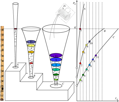
Figure 4: Maximin vase filling.

The jammer’s optimal strategy is presented in Theorem 2 below. The theorem is complemented by the numerical algorithm and the intuition-building analogy that follows its proof.

Theorem 2

It is optimal for the jammer to make $J_{M}(\mathbf{h})$ satisfy the power constraint with equality. The optimal jammer strategy for allocating power across frames is to increase the required transmitter power, starting with those frames whose channel realizations exhibit the steepest instantaneous slope of the characteristic $\mathscr{P}_{M}(J_{M})$ curve. The jamming power should be allocated such that the required transmitter power over each channel realization where the jammer is present does not exceed a pre-defined level $K$.

The optimal value for $K$ that maximizes the outage probability can be found numerically, by exhaustive search in a compact interval of the positive real line.

Proof:

Our proof takes a contradictory approach. Instead of deriving the optimal strategy defined above in a direct manner, we show instead that any other strategy not satisfying the theorem’s requirements is suboptimal. Let $\mathscr{S},\mathscr{X}\subset\mathbb{R}_{+}^{M}$ denote the sets of channel realizations over which the transmitter and the jammer are present, respectively.

Suppose the jammer picks a certain strategy $J_{M}(\mathbf{h})$. Since the transmitter’s strategy is predictable, the jammer already knows the transmitter’s optimal strategy. Under this optimal strategy, the transmitter picks a set of frames $\mathscr{S}$ over which it will invest non-zero power. This choice also results in a maximum level of required transmitter power that will actually be matched by the transmitter. Denote this level by $K$.

Since the transmitter’s strategy is the optimal response to the jammer’s strategy, the required transmitter power should be larger than or equal to $K$ over the set of frames $\mathscr{X}\setminus\mathscr{S}$ where the jammer jams, but the transmitter does not afford to transmit. Otherwise, the transmitter would be wasting power and its strategy would not be optimal.

But since the jammer knows the transmitter’s strategy, and knows that the transmitter will not transmit over $\mathscr{X}\setminus\mathscr{S}$, its optimal strategy should make the required transmitter power over $\mathscr{X}\setminus\mathscr{S}$ at most equal to $K$. Otherwise the jammer would be wasting power.

We have seen how the jammer’s power should be distributed over $\mathscr{X}\setminus\mathscr{S}$. Next we show that if the jammer’s power allocation over $\mathscr{S}\bigcap\mathscr{X}$ is not done according to the theorem, the jammer’s strategy is not optimal. For this, we assume that the jammer’s strategy does not satisfy the theorem’s requirements, and provide a method of improvement (i.e. we prove sub-optimality).

If the theorem is not satisfied, than there exist two sets $\mathscr{A},\mathscr{B}\subset\mathscr{S}\bigcap\mathscr{X}$ of non-zero $\mathfrak{m}$-measure such that$\frac{dP_{M}(\mathbf{h}_{1})}{dJ_{M}}>\frac{dP_{M}(\mathbf{h}_{2})}{dJ_{M}}~{}\forall~{}\mathbf{h}_{1}\in\mathscr{A}~{}\textrm{and}~{}\mathbf{h}_{2}\in\mathscr{B}$, and such that the required $P_{M}$ is less than $K$ on $\mathscr{A}$ and $J_{M}>0$ on $\mathscr{B}$.

Consider a small enough amount of jamming power $\delta J_{M}$, such that, for any channel realization $\mathbf{h}\in\mathscr{A}\bigcup\mathscr{B}$, we can modify the jamming power by $\delta J_{M}$ without changing the slope of the $\mathscr{P}_{M}(J_{M})$ curve. Subtracting $\delta J_{M}$ from all frames in $\mathscr{B}$, the jammer obtains the excess power $\delta J_{M}m(\mathscr{B})$, which it can allocate uniformly over $\mathscr{A}$. The jammer’s total average power remains unchanged. However, the required transmitter power over $\mathscr{A}\bigcup\mathscr{B}$ is increased (because the slopes of the $\mathscr{P}_{M}(J_{M})$ curves corresponding to $\mathscr{A}$ are all larger than the slopes of the $\mathscr{P}_{M}(J_{M})$ curves corresponding to $\mathscr{B}$), and thus the modification results in a larger probability of outage.

There exists a closed interval $[0,K_{max}]\in\mathbb{R}_{+}$ which includes the optimal value of $K$. This observation is vital to the existence of a numerical algorithm that searches for the optimal $K$. Once such an interval has been set, we can fix the desired resolution and calculate the numerical complexity of the algorithm. We next show how the upper limit $K_{max}$ of this interval can be found. Consider the set of channel realizations $\mathscr{S}_{0}$ where the transmitter is active when the jammer does not interfere with the transmission. Next, find the value $K_{max}$ for which, when the jammer allocates its power $\mathcal{J}$ according to the rules of the theorem, we obtain a set $\mathscr{X}_{0}\subset\mathbb{R}^{M}_{+}\setminus\mathscr{S}_{0}$. This means that the jammer’s strategy under any $K\geq K_{max}$ has no influence upon the transmitter’s strategy. Note that such a finite $K_{max}$ can be found whenever $\mathbb{R}^{M}_{+}\setminus\mathscr{S}_{0}$ has non-zero $\mathfrak{m}$-measure. ∎

The algorithm in Table I which we used in generating our numerical results in Subsection III-C helps shed more light into the practicality of Theorem 2. In the description of the algorithm, we assume discrete jamming power levels $J_{M}^{k}$ with $k=0,1,\ldots$ and $J_{M}^{0}=0$, as well as a discrete and finite channel coefficient space. As a consequence, there exists a finite number of $\mathscr{P}_{M}(J_{M})$ curves, each characterizing one possible channel realization, and each completely determined by a finite vector whose components are the values of $\mathscr{P}_{M}(J_{M}^{k})$ for that particular channel realization.

An intuitive description of the technique is given in Figure 4. Consider the problem where the jammer has to pour water in a number of vases (a vase for each possible channel realization). The shape of each vase is such that the vertical section of its wall produces a concave curve similar to the corresponding $\mathscr{P}_{M}(J_{M})$ curve. The jammer can afford to spend a certain volume of water. The jammer wants to “annoy” the transmitter, which is deeply concerned with the sum of the heights that the water levels reach in the vases. Hence, the jammer tries to use its available volume of water, such that the sum of the water levels’ heights is maximized. However, the jammer cannot pour all the water in the thinnest vase, because then the transmitter might just ignore that vase. Instead, the jammer has to set a height limit $K$ which it should not exceed. The jammer pours the water a cup at a time, starting with the vase in which a cup of water rises the water level the quickest. In Figure 4, the order of adding cups to the vases is shown by numerals from $1$ to $11$. The first cup is poured into the thinnest vase (vase $A$) and incidentally reaches the level $K$. Thus, no more water should be added to vase $A$. The next three cups are added to vase $B$, and then the next five cups to vase $C$. Then the jammer returns to vase $B$, and adds another cup, for this increases the water level more than it would increase the level in vase $C$. Finally, the last available cup is added to vase $C$. The way the numerical algorithm works is illustrated in the right part of Figure 4.

TABLE I: Numerical algorithm for deriving the maximin solution.

Let $\mathbf{P}$ denote a matrix with each row representing one of the vectors $\mathscr{P}_{M}(J_{M}^{k})$, for different channel realizations $\mathbf{h}$. Let $P_{req}$ be the vector of required powers for the different frames. The initial $P_{req}$ is set equal to the first column of $\mathbf{P}$. Let $K_{max}$ be the upper limit when searching for the optimal $K$.

Initialize $K=0$.

while $K\leq K_{max}$

$p_{T}=0$.

Let $L$ be an index vector, the same size as $P_{req}$.

Initialize all components of $L$ to be equal to $1$.

We have the relationship $P_{req}(j)=\mathbf{P}(j,L(j))$.

% Jx strategy:

The amount of jamming power spent at each step is accumulated into the variable $J_{c}$.

while Jx power constraint is satisfied ($J_{c}\leq\mathcal{J}$)

Find row $j$ of $\mathbf{P}$ with the largest difference

between components $L(j)+1$ and $L(j)$,

and such that $\mathbf{P}(j,L(j)+1)\leq K$.

$P_{req}(j)=\mathbf{P}(j,L(j)+1)$.

$L(j)=L(j)+1$.

Weigh $J_{M}^{j}$ by probability of row $j$ and add to $J_{c}$.

end

% Tx strategy (Tx picks frames where required power is minimum first)

The amount of transmitter power spent at each step is simulated into the variable $P_{c}$.

while Tx power constraint is satisfied ($P_{c}\leq\mathcal{P}$)

Pick the least component of $P_{req}$.

Add probability of corresponding frame to $p_{T}$.

Add value of component, weighted by

probability above, to $P_{c}$.

Delete component from $P_{req}$.

end

$P_{out}(K)=1-p_{T}$

Increment K.

end

Select K that produces the largest $P_{out}$.

The Minimax Solution

In Theorem 3 we showed that given the transmitter’s and the jammer’s powers $P_{M}$ and $J_{M}$ allocated to a frame, the optimal strategies for distributing these powers inside the frame are identical for the minimax and the maximin problems. Hence, by rotating the $\mathscr{P}_{M}(J_{M})$ plane, we get the characteristic $\mathscr{J}_{M}(P_{M})$ curves for the minimax problem.

We already know that given the transmitter’s strategy, the optimal way of allocating the jammer’s power is such that outage is first induced on the frames that require the least amount of jamming power.

The transmitter’s optimal strategy is presented in the following theorem, which is complemented by the numerical algorithm and the analogy that follows its proof.

Theorem 3

It is optimal for transmitter to make $P_{M}(\mathbf{h})$ satisfy the long-term power constraint with equality. The optimal transmitter power allocation across frames is to increase the required jamming power up to some pre-defined level $K$, starting with those frames on which the required transmitter power to achieve this goal is least.

The optimal value for $K$ that minimizes the outage probability can be found numerically by exhaustive search.

Proof:

As in the case of Theorem 2, we take a contradictory approach. Instead of directly deriving the optimal strategy defined above, we show that any other strategy not satisfying the theorem’s requirements is suboptimal. Recall that $\mathscr{S}~{}\textrm{and}~{}\mathscr{X}\subset\mathbb{R}_{+}^{M}$ denote the sets of channel realizations over which the transmitter and the jammer are present, respectively.

Suppose the transmitter picks a certain strategy $P_{M}(\mathbf{h})$. Since the jammer’s strategy is predictable, the transmitter already knows the jammer’s optimal strategy. Under this optimal strategy, the jammer should pick a set of frames $\mathscr{X}$ over which it will invest non-zero power. This choice also results in a maximum level of required jamming power that will actually be matched by the jammer. Denote this level by $K$.

Since the jammer’s strategy is optimal, the required jamming power outside the set $\mathscr{X}$ should be larger than or equal to $K$. Otherwise, the jammer would be wasting power and hence its strategy would not be optimal.

But since the transmitter knows the jammer’s strategy, it also knows that the jammer will not be present over $\mathscr{S}\setminus\mathscr{X}$, so the transmitter should make the required jamming power over $\mathscr{S}\setminus\mathscr{X}$ at most equal to $K$. Otherwise the transmitter would be wasting power. Hence, over $\mathscr{S}\setminus\mathscr{X}$ the transmitter should allocate power such that the required jamming power is equal to $K$.

Next we show that if the transmitter’s power allocation over $\mathscr{S}\bigcap\mathscr{X}$ is not done according to the theorem, the transmitter’s strategy is not optimal. For this, we assume that the transmitter’s strategy does not satisfy the theorem’s requirements, and provide a method of improvement (i.e. we prove sub-optimality).

If the theorem is not satisfied, than there exist two sets $\mathscr{A},\mathscr{B}\subset\mathscr{S}\bigcap\mathscr{X}$ of non-zero $\mathfrak{m}$-measure such that $P_{M}(\mathbf{h}_{1},K)<P_{M}(\mathbf{h}_{2},K)~{}\forall~{}\mathbf{h}_{1}\in\mathscr{A}~{}\textrm{and}~{}\mathbf{h}_{2}\in\mathscr{B}$, and such that the required $J_{M}$ is less than $K$ on $\mathscr{A}$ and $J_{M}>0$ on $\mathscr{B}$ cannot be part of the minimax solution. Denote the original transmitter power allocation functions over $\mathscr{A}$ and $\mathscr{B}$ by $P_{M,0}^{A}(\mathbf{h})$ and $P_{M,0}^{B}(\mathbf{h})$ respectively.

For any $\mathbf{h}_{1}\in\mathscr{A},~{}\mathbf{h}_{2}\in\mathscr{B}$ and $J_{M,1},J_{M,2}<K$, we have:

$$\frac{K-J_{M,1}}{P_{M}(\mathbf{h}_{1},K)-P_{M}(\mathbf{h}_{1},J_{M,1})}\stackrel{{\scriptstyle a)}}{{\geq}}\frac{K}{P_{M}(\mathbf{h}_{1},K)}>{}$$

$${}\stackrel{{\scriptstyle b)}}{{>}}\frac{K}{P_{M}(\mathbf{h}_{2},K)}\stackrel{{\scriptstyle c)}}{{\geq}}\frac{J_{M,2}}{P_{M}(\mathbf{h}_{2},J_{M,2})},$$ (39)

where both $a)$ and $c)$ follow from the convexity of $\mathscr{J}_{M}(P_{M})$ – Proposition 5 – and $b)$ follows from the assumption in the beginning of this proof.

If the transmitter cuts off transmission over a subset $\mathscr{B}^{\prime}\subset\mathscr{B}$, it obtains the excess power $\int_{\mathscr{B}^{\prime}}P_{M}(\mathbf{h})dm(\mathbf{h})$, which it can allocate to a subset $\mathscr{A}^{\prime}\subset\mathscr{A}$ such that the required $J_{M}$ is equal to $K$ over $\mathscr{A}^{\prime}$, i.e.

$$\int_{\mathscr{B}^{\prime}}P_{M,0}^{B}(\mathbf{h})dm(\mathbf{h})=\int_{\mathscr{A}^{\prime}}\left[P_{M}(\mathbf{h},K)-P_{M,0}^{A}(\mathbf{h})\right]dm(\mathbf{h})$$ (40)

Replacing $P_{M}(\mathbf{h}_{1},J_{M,1})$ by $P_{M,0}^{A}(\mathbf{h})$ and $P_{M}(\mathbf{h}_{2},J_{M,2})$ by $P_{M,0}^{B}(\mathbf{h})$ in (III-B), we see the transmitter improves its strategy by forcing the jammer to allocate more power to the set $\mathscr{A}\bigcup\mathscr{B}$, and hence decreases the probability of outage. Note that since $\mathscr{B}^{\prime}\subset\mathscr{S}\bigcap\mathscr{X}$, the set $\mathscr{B}^{\prime}$ is in outage, regardless of whether the transmitter is present or not. Thus, transmitter does not increase $P_{out}$ by cutting off transmission on $\mathscr{B}^{\prime}$.

There exists a closed interval $[0,K_{max}]\in\mathbb{R}_{+}$ which includes the optimal value of $K$. As in the maximin case, the existence of such a closed interval is required for constructing a numerical algorithm that searches for the optimal $K$. The upper limit $K_{max}$ of this interval can be found and updated as follows. First solve the problem for an arbitrarily chosen $K_{0}$, and determine the set $\mathscr{S}_{0}\setminus\mathscr{X}_{0}$ over which the transmitter achieves reliable communication. We can set $K_{max}$ equal to the value of $K$ that yields a set $\mathscr{S}$ of the same $\mathfrak{m}$-measure as the set $\mathscr{S}_{0}\setminus\mathscr{X}_{0}$. Note that if $K$ is increased over this $K_{max}$, the outage probability is at least as large as that obtained for $K=K_{0}$ (and hence $K_{0}$ is a better choice). ∎

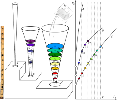
Figure 5: Minimax vase filling.

The algorithm in Table II which we used for our numerical results in Subsection III-C illustrates the application of Theorem 3. In the description of the algorithm, we assume discrete jamming power levels $J_{M}^{k}$ with $k=0,1,\ldots$ and $J_{M}^{0}=0$, as well as a discrete and finite channel coefficient space. As a consequence, there exists a finite number of $\mathscr{P}_{M}(J_{M})$ curves, each characterizing one possible channel realization, and each completely determined by a finite vector whose components are the values of $\mathscr{P}_{M}(J_{M}^{k})$ for that particular channel realization.

A description of the technique is given in Figure 5, using the same vase analogy as in the maximin case. This time, the transmitter does the pouring. Its obsession with the sum of the heights of the water levels imposes a constraint on this sum. Under this constraint, the transmitter wants to use as much of the jammer’s water as possible. That is, the transmitter attempts to maximize the volume of water that can be accommodated by the vases, under the constraint that the sum of the water levels’ heights is less than some given value. Moreover, if the transmitter pours water only in the thickest vase, it might not feel that it did enough damage to the jammer. Thus, the transmitter needs to set a limit $K$. The optimal strategy is to fill (up to volume level $K$) the thickest vase first (note that “thickest” refers to the fact that when filled up to volume level $K$, the vase displays the lowest water level height, thus “thickest” is defined with respect to $K$). The order in which the transmitter adds cups of water to the vases is depicted in Figure 5 by numerals from $1$ to $12$. The way the numerical algorithm works is illustrated in the right part of Figure 5.

TABLE II: Numerical algorithm for deriving the minimax solution.

Let $\mathbf{P}$ denote the matrix with rows representing the $\mathscr{P}_{M}(J_{M}^{k})$ vectors for different channel realizations $\mathbf{h}$. Let $K_{max}$ be value where searching for the optimal $K$ stops.

Initialize $K=0$.

while $K\leq K_{max}$

% Tx strategy:

The amount of transmitter power spent at each step is accumulated into the variable $P_{c}$.

Initialize $K=J_{M}^{k}$.

Initialize $P_{c}=0,~{}p_{T}=0$.

while Tx power constraint is satisfied ($P_{c}\leq\mathcal{P}$)

Find row $j$ of $\mathbf{P}$ with least $k$-th component.

Add probability of row $j$ to $p_{T}$.

Add value of the $k$-th component, weighted

by the probability above, to $P_{c}$.

Delete row $j$ from matrix $\mathbf{P}$.

end

% Jx strategy (Jx jams frames where Tx is present, randomly, until it reaches its power constraints):

$p_{J}=\frac{\mathcal{J}}{K}$.

$P_{out}(K)=p_{T}-p_{J}$.

Increment $K$.

end

Select K that produces the least $P_{out}$.

Particular case: $M=1$

For this simple scenario, there is no second level of power allocation. All frames consist of only one block, and the $P_{M}(J_{M})$ curves have the particular affine form with parameter $h$ (the squared channel coefficient corresponding to this block):

$$P_{M}=\frac{\exp(R)-1}{h}(J_{M}+\sigma_{N}^{2}).$$ (41)

Since the slopes of the $P_{M}(J_{M})$ curves are constant with $J_{M}$ and the frames with smaller values of the channel coefficients have larger characteristic slopes, we can easily particularize Theorems 2 and 3.

With the same notation $\mathscr{X}\subset\mathbb{R}_{+}$ for the set of channel realizations over which the jammer invests non-zero power and $\mathscr{S}\subset\mathbb{R}_{+}$ for the set of channel realizations over which the transmitter uses non-zero power, we can now define the optimal power allocation strategies.

For the maximin scenario, The jammer should deploy some $J_{M}(h)$ over $\mathscr{X}$ such that the required $P_{M}(h)$ is constant over the whole interval $\mathscr{X}$. The purpose of the jammer being active over $\mathscr{X}\setminus\mathscr{S}$ is to ”intimidate” the transmitter. The transmitter plays second, and hence takes advantage of the jammer’s weaknesses. It always chooses to be active on the subset of $\mathscr{X}$ on which the required $P_{M}(h)$ is least. This is why the optimal jammer strategy is to display no weakness, i.e. to make $P_{M}(h)$ constant over $\mathscr{X}$. These considerations are formalized in Proposition 6 below.

Proposition 6

In the maximin scenario, the jammer should adopt such a strategy as to make the transmitter’s best choice of $\mathscr{S}$ intersect $\mathscr{X}$ on the the left-most part of $\mathscr{S}$, and the required transmitter power equal to some constant $K$ on $\mathscr{X}\bigcap\mathscr{S}$ and to $(c-1)\sigma_{N}^{2}/h$ on $\mathscr{S}\setminus\mathscr{X}$.

Transmitting $J_{M}(h)$, satisfying the power constraint with equality, such that the transmitter power required for reliable communication is $P_{M}(h)=K,\forall h\in[h_{1}^{*},h_{2}^{*}]$, and $P_{M}(h)=(c-1)\sigma_{N}^{2}/h,\forall h\in[0,\infty)\setminus(h_{1}^{*},h_{2}^{*}]$, for some $h_{1}^{*}<h_{2}^{*}\in\mathbb{R}_{+}$ and some constant $K\in\mathbb{R}_{+}\bigcup\{\infty\}$ is an optimal jammer strategy for the maximin problem. (Note that $P_{M}(h)$ should be continuous at $h_{1}^{*}$.)

The values $K,~{}h_{1}^{*}$ and $h_{2}^{*}$ that maximize the outage probability can be found by solving the following problem:

Find $$\min_{K}\int_{h_{0}}^{\infty}f(h)dh$$, where

$$h_{0} \int_{h_{0}}^{h_{2}}Kf(h)dh+\int_{h_{2}}^{\infty}\frac{c-1}{h}\sigma_{N}^{2}f(h)dh=\mathcal{P}$$ is given by , (42)

$$h_{1} h_{1}=\frac{c-1}{K}\sigma_{N}^{2}$$ is given by , (43)

$$\textrm{and $h_{2}$ is given by $\int_{h_{1}}^{h_{2}}\left(\frac{hK}{c-1}-\sigma_{N}^{2}\right)f(h)dh=\mathcal{J}$}.$$ (44)

$\blacksquare$

The power allocation is depicted in Figure 6. The convex decreasing curve represents the original required transmitter power, without the presence of a jammer and satisfies the equation $P_{M}=(c-1)\sigma_{N}^{2}/h$. Notice how by picking some $K$, we can determine $h_{1}$, $h_{2}$ and $h_{0}$ (in this order), and then find the probability of outage as $P_{out}(h_{1})=1-\mathfrak{m}[(h_{0},\infty)]$. The optimal $K$, resulting in $h_{1}^{*}$, $h_{2}^{*}$ and $h_{0}^{*}$, is the one minimizing the $\mathfrak{m}$-measure of the set $(h_{0},\infty)$.

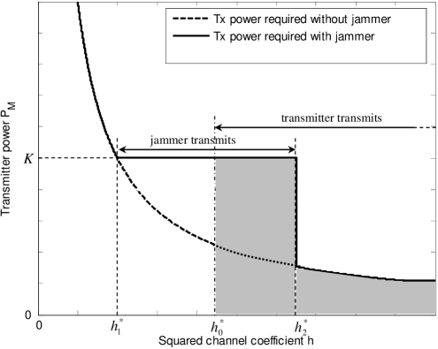
Figure 6: Maximin solution for $M=1$ - power distribution between frames

For the minimax scenario the jammer will not transmit any power over a frame if outage is not going to be induced or if the transmitter is not present, i.e. $\mathscr{X}\subset\mathscr{S}$. The jammer will start allocating power to the frames over which an outage is easiest to induce, and go on with this technique until the average power reaches the limit set by its power constraint. Obviously, the jammer prefers the frames for which the required $J_{M}(h)$ is less. The optimal transmitter’s strategy is to allocate its power such that the required $J_{M}(h)$ is constant on the whole set $\mathscr{S}$, and hence to display no weakness.

These considerations are formalized in Proposition 7 below.

Proposition 7

For the minimax scenario, the transmitter’s optimal way to allocate its power is to make the required jamming power remain equal to some constant $K$ on all of $\mathscr{X}$. Transmitting $P_{M}(h)$, satisfying the power constraint with equality, such that the required $J_{M}(h)$ equals $K$ for $h\in[h_{x}^{*},\infty)$, and $J_{M}(h)=0~{}\forall h\in[0,h_{x}^{*})$, for some $h_{x}^{*}\in\mathbb{R}_{+}$, is an optimal transmitter strategy for the minimax problem. The values $K$ and $h_{x}^{*}$ that minimize the outage probability can be found by solving the following problem numerically:

Find $$\max_{K}\int_{h_{0}}^{\infty}f(h)dh$$, where

$$h_{0} \int_{h_{x}}^{h_{0}}Kf(h)dh=\mathcal{J}$$ is given by , (45)

$$\textrm{$h_{x}$ is given by $\int_{h_{x}}^{\infty}\frac{(c-1)(K+\sigma_{N}^{2})}{h}f(h)dh=\mathcal{P}$}.$$ (46)

$\blacksquare$

The numerical problem is described in Figure 7. Notice how by picking some $K$, we can determine $h_{x}$ and $h_{0}$ (in this order), and then find the probability of outage as $P_{out}(h_{1})=1-\mathfrak{m}[(h_{0},\infty)]$. The optimal $K$, resulting in $h_{x}^{*}$ and $h_{0}^{*}$, is the one maximizing the $\mathfrak{m}$-measure of the set $(h_{0},\infty)$. Note that the jammer does not necessarily have to jam on an interval of the form $[h_{x},h_{0}]$. The jammer’s choice space (the set of frames out of which the jammer picks its set $\mathscr{X}$) is an indifferent one, i.e. the jammer can randomly pick $\mathscr{X}\subset[h_{x},\infty)$ as long as its measure satisfies $K\mathfrak{m}(\mathscr{X})=\mathcal{J}$. However, for the purpose of computing the outage probability, the representation of $\mathscr{X}$ as an interval is convenient and incurs no loss of generality.

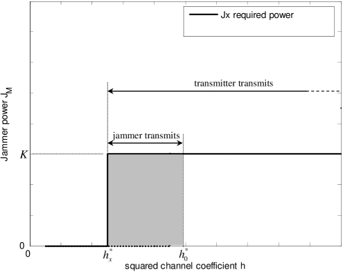
Figure 7: Minimax solution for $M=1$ - power distribution between frames

III-C Numerical Results

We have computed the outage probabilities for both minimax and maximin problems when $M=1$ and $M=2$. The channel coefficients are assumed i.i.d. exponentially distributed with parameter $\lambda=1/6$. Figure 8 shows the outage probability vs. the maximum allowable average transmitter power $\mathcal{P}$ for fixed $\mathcal{J}=10$ when $R=1$.

For comparison purposes, we also plotted the results for the case when $M=\infty$, which are readily available from Part I of this paper [1].

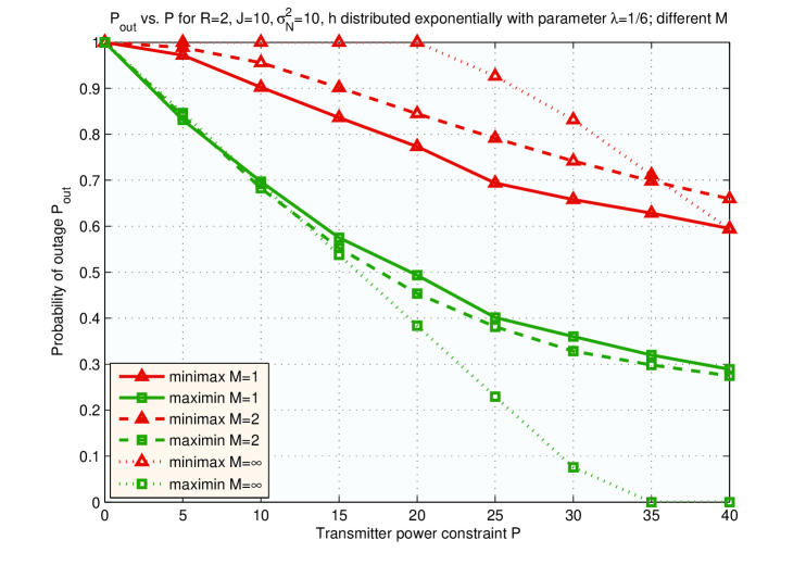
Figure 8: Outage probability vs. $\mathcal{P}$ for $M=1$ and $M=2$ and $M\to\infty$ when $\mathcal{J}=10$ – minimax and maximin cases. We take $R=2$.

Numerical results demonstrate a sharp difference between the minimax solutions and the maxmin solutions, which demonstrates the non-existence of Nash-equilibria of pure strategies for our two-person zero-sum game with full CSI.

Note the behavior of the outage probability when the number of blocks per frame $M$ is increased. At low transmitter powers, the increase of $M$ produces an increase in the outage probability for both the minimax, and the maximin scenarios.

On the contrary, at higher transmitter powers a lower outage probability is obtained for both the minimax and the maximin cases when $M$ is larger. This behavior can be summarized as follows: the more powerful player will use the available diversity to its own advantage.

IV CSI Available to All Parties. Jamming Game with Long-Term Power Constraints: Mixed Strategies

We have already seen that the maximin and minimax solutions of the jamming game when only pure strategies are allowed do not agree, and thus our game has no Nash equilibrium of pure strategies. However, recall that the solution of the minimax problem with pure strategies can often be a good characterization of a practical jamming situation (e.g. when the jammer does not transmit unless it senses that the transmitter is on) and can always serve as a lower bound on the system’s performance.

This aside, a Nash equilibrium is still the preferred characterization of jamming games, and since such an equilibrium exists for our problem only when mixed strategies are allowed, the current section is dedicated to the derivation of such a saddlepoint.

Unlike the fast fading scenario of [1], the frames in our slow-fading parallel-channels model are not equivalent. Each frame is characterized by a different realization of the channel vector $\mathbf{h}$. This is why our present scenario is even more involved than the one in [1], and requires three levels of power control instead of two.

As before, our approach to the problem is a contradictory one. We study the power control levels starting with the “finest” one, and show that if our conditions for power allocations are not satisfied, then the strategy is suboptimal. The reason why an additional (third) level of power control appears here is a combination of the facts that we study mixed strategies and the frames are not all equivalent as in [1]. Namely, to cover all possible probabilistic strategies, we need to dedicate a level of power control to the power allocation between frames with the same channel realizations (i.e. equivalent frames) and an additional level of power control for the power allocation between frames with different channel realizations. Along with the power allocation within frames, these problems cover all possible cases.

IV-A Power allocation within a frame

The third level of power control deals with the optimal power allocation between the blocks in a frame, once the transmitter is given the channel vector $\mathbf{h}$ characterizing the frame and allocated power $P_{M}$, and the jammer is given the channel vector and its allocated power $J_{M}$.

At this point, the third level of power control resembles the two-player, zero-sum game of (9) and (12) having the mutual information calculated over a frame $I_{M}$ as cost function. However, none of the players knows the other player’s constraints, because $(P_{M},J_{M})$ is a random event. Theorem 4 below provides the optimal transmitter/jammer strategies for power allocation within a frame.

Theorem 4

Given a frame with channel vector $\mathbf{h}$ and a realization $(p_{M},j_{M})$ of $(P_{M},J_{M})$, let $\mathscr{P}_{M}(j_{M})$ denote the solution of Problem 1 in Section III with $J_{M}=j_{M}$, and $\mathscr{J}_{M}(p_{M})$ denote the solution of Problem 2 in Section III with $P_{M}=p_{M}$.

The transmitter’s optimal strategy is the solution of the game in (9) and (12), where the jammer is constrained to $\frac{1}{M}\sum_{m=1}^{M-1}J_{m}\leq\mathscr{J}_{M}(p_{M})$ and the transmitter is constrained to $\frac{1}{M}\sum_{m=1}^{M-1}P_{m}\leq p_{M}$. The jammer’s optimal strategy is the solution of the game in (9) and (12), where the transmitter is constrained to $\frac{1}{M}\sum_{m=1}^{M-1}P_{m}\leq\mathscr{P}_{M}(j_{M})$ and the jammer is constrained to $\frac{1}{M}\sum_{m=1}^{M-1}J_{m}\leq j_{M}$.

Proof:

The proof is very similar to the proof of Theorem 5 of [1] and is deferred to Appendix C ∎

IV-B Power allocation between frames with the same channel vector

Due to the form of the optimal second level power allocation strategies described in the previous subsection, the probability that a given frame is in outage can be expressed as

$$P_{out,\mathbf{h}}=Pr\{J_{M}\geq\mathscr{J}_{M}(P_{M})\}={}$$

$${}=1-Pr\{P_{M}\geq\mathscr{P}_{M}(J_{M})\},$$ (47)

where $P_{M}(j_{M})$ is the strictly increasing, unbounded and concave function (see Proposition 5) that characterizes the frame. Note that a pair of strategies can only be optimal if $P_{out,\mathbf{h}}$ above is the Nash equilibrium of a jamming game played over the frames characterized by the same channel vector $\mathbf{h}$. This means that if the transmitter and jammer decide to allocate powers $P_{M,\mathbf{h}}$ and $J_{M,\mathbf{h}}$ respectively to frames with channel vector $\mathbf{h}$, they should not allocate the same amount of power to each of these frames. Instead, they should use power levels given by the realizations of two random variables $P_{M}$ and $J_{M}$ with distribution functions $\left(F_{P}(p_{M}),F_{J}(j_{M})\right)$ given in the following theorem.

Theorem 5

The unique Nash equilibrium of mixed strategies of the two-player, zero-sum game with average power constraints described by

$$\min_{F_{P}(p_{M}):\mathbf{E}_{F_{P}}P_{M}\leq P_{M}(\mathbf{h})}\max_{F_{J}(j_{M}):\mathbf{E}_{F_{J}}J_{M}\leq J_{M}(\mathbf{h})}P_{out,\mathbf{h}},$$ (48)

where $\mathbf{E}_{F_{P}}$ and $\mathbf{E}_{F_{J}}$ denote expectations with respect to the distributions $F_{P}(p_{M})$ and $F_{J}(j_{M})$, is attained by the pair of strategies $\left(F_{P}(p_{M}),F_{J}(j_{M})\right)$ satisfying:

$$F_{P}(\mathscr{P}_{M}(y))\sim k_{p}\mathbb{U}([0,2v])(y)+(1-k_{p})\Delta_{0}(y),$$ (49)

$$F_{J}(\mathscr{J}_{M}(x))\sim k_{j}\mathbb{U}([0,J_{M}(2v)])(x)+(1-k_{j})\Delta_{0}(x),$$ (50)

where $\mathbb{U}([r,t])(\cdot)$ denotes the CDF of a uniform distribution over the interval $[r,t]$, and $\Delta_{0}(\cdot)$ denotes the CDF of a Dirac distribution (i.e. a step function), and the parameters $k_{p},k_{j}\in[0,1]$ and $v\in[\max\{J_{M,\mathbf{h}},\mathscr{J}_{M}(P_{M,\mathbf{h}})/2\},\infty)$ are uniquely determined from the following steps:

1. Find the unique value $v_{0}$ which satisfies:

   $$P_{M,\mathbf{h}}J_{M,\mathbf{h}}=[\mathscr{P}_{M}(2v_{0})-P_{M,\mathbf{h}}](2v_{0}-J_{M,\mathbf{h}}).$$ (51)

2. Compute $S(v_{0})=\int_{0}^{2v_{0}}\mathscr{P}_{M}(y)dy-2v_{0}P_{M,\mathbf{h}}$.

3. If $S(v_{0})<0$, then $v$ is the unique solution of

   $$\int_{0}^{2v}\mathscr{P}_{M}(y)dy-2vP_{M,\mathbf{h}}=0,$$ (52)

   $$k_{p}=1$$ (53)

   and

   $$k_{j}=\frac{J_{M,\mathbf{h}}\mathscr{P}_{M}(2v)}{2v[\mathscr{P}_{M}(2v)-P_{M,\mathbf{h}}]}.$$ (54)

4. If $S(v_{0})=0$ then $v=v_{0}$, $k_{p}=k_{j}=1$.

5. If $S(v_{0})>0$, then $v$ is the unique solution of

   $$\int_{0}^{2v}\mathscr{P}_{M}(y)dy-\mathscr{P}_{M}(2v)(2v-J_{M,\mathbf{h}})=0,$$ (55)

   $$k_{p}=\frac{2vP_{M,\mathbf{h}}}{\mathscr{P}_{M}(2v)[2v-J_{M,\mathbf{h}}]}$$ (56)

   and

   $$k_{j}=1.$$ (57)

Proof:

The proof follows directly from Theorem 9 in Appendix III of [1], by substituting $x=P_{M}$, $y=J_{M}$, $g(y)=\mathscr{P}_{M}(y)$, $g^{-1}(x)=\mathscr{J}_{M}(x)$, $a=P_{M,\mathbf{h}}$ and $b=J_{M,\mathbf{h}}$. It is also interesting to note that the condition $\int_{0}^{b}g(y)dy<\int_{g(b)}^{\infty}g^{-1}(x)dx$ is satisfied because $\mathscr{P}_{M}(y)$ is unbounded. ∎

Particular case: $M=1$

For $M=1$ the first (intra-frame) level of power control is inexistent. For a given channel realization $h$ we can readily derive the affine function $P_{M}(j_{M})$ in (IV-B) as

$$P_{M}(j_{M})=\frac{c-1}{h}(j_{M}+\sigma_{N}^{2})$$ (58)

where $c=\exp(R)$. If we use the particularization of the general solution of Theorem 5 to affine functions, as in the last part of Appendix III of [1], we obtain the outage probability as

$$P_{out,h}=1-\frac{\frac{hP_{M}(h)}{c-1}}{J_{M}(h)\left[1+\sqrt{1+2\frac{\sigma_{N}^{2}}{J_{M}(h)}}\right]+\sigma_{N}^{2}}$$

$$\textrm{if}~{}~{}\frac{hP_{M}(h)}{c-1}\leq\frac{1}{2}J_{M}(h)\left[1+\sqrt{1+2\frac{\sigma_{N}^{2}}{J_{M}(h)}}\right]+\sigma_{N}^{2},$$ (59)

and

$$P_{out,h}=\frac{\frac{1}{2}J_{M}(h)}{\frac{hP_{M}(h)}{c-1}-\sigma_{N}^{2}}$$

$$\textrm{if}~{}~{}\frac{hP_{M}(h)}{c-1}>\frac{1}{2}J_{M}(h)\left[1+\sqrt{1+2\frac{\sigma_{N}^{2}}{J_{M}(h)}}\right]+\sigma_{N}^{2}.$$ (60)

The transmitter and jammer strategies that achieve these payoffs are such that

$$F_{P}(x)\sim k_{p}\mathbb{U}([\frac{c-1}{h}\sigma_{N}^{2},2v\frac{c-1}{h}+\frac{c-1}{h}\sigma_{N}^{2}])(x)+$$

$$+(1-k_{p})\Delta_{0}(x),$$

$$F_{J}(y)\sim\frac{2v}{2v+\sigma_{N}^{2}}k_{j}\mathbb{U}([0,2v])(y)+(1-\frac{2v}{2v+\sigma_{N}^{2}}k_{j})\Delta_{0}(y).$$

The parameters $k_{p},k_{j}\in[0,1]$ and $v\in[\max\{J_{M}(h),\mathscr{J^{\prime}}_{M}(P_{M}(h))/2\},\infty)$ are uniquely determined from the following steps:

1. If

   $$\frac{hP_{M}(h)}{c-1}\leq\frac{1}{2}J_{M}(h)\left[1+\sqrt{1+2\frac{\sigma_{N}^{2}}{J_{M}(h)}}\right]+\sigma_{N}^{2},$$ (61)

   then

   $$v=\frac{1}{2}J_{M}(h)\left[1+\sqrt{1+\frac{2\sigma_{N}^{2}}{J_{M}(h)}}\right],$$ (62)

   $$k_{p}=\frac{2vP_{M}(h)}{\frac{c-1}{h}(2v+\sigma_{N}^{2})(2v-J_{M}(h))}$$ (63)

   and

   $$k_{j}=1.$$ (64)

2. If

   $$\frac{hP_{M}(h)}{c-1}>\frac{1}{2}J_{M}(h)\left[1+\sqrt{1+2\frac{\sigma_{N}^{2}}{J_{M}(h)}}\right]+\sigma_{N}^{2},$$ (65)

   then

   $$v=\frac{P_{M}(h)-\frac{c-1}{h}\sigma_{N}^{2}}{\frac{c-1}{h}},$$ (66)

   $$k_{p}=1$$ (67)

   and

   $$k_{j}=\frac{\frac{c-1}{h}J_{M}(h)(2P_{M}(h)-\frac{c-1}{h}\sigma_{N}^{2})}{2(P_{M}(h)-\frac{c-1}{h}\sigma_{N}^{2})^{2}}.$$ (68)

The special form of this solution will be used in the next subsection to derive the overall Nash equilibrium of the mixed strategies game for $M=1$.

IV-C Power allocation between frames with different channel vectors

In the previous subsections we have described the optimal power control strategies for given particular channel realization $\mathbf{h}$, and transmitter and jammer power levels $P_{M,\mathbf{h}}$ and $J_{M,\mathbf{h}}$ respectively. The first level of power control,which is the subject of this subsection, deals with allocating the powers specified by the transmitter and jammer average power constraints $\mathcal{P}$ and $\mathcal{J}$ between different channel vectors. In other words, we are now concerned with solving the problem

$$\min_{P_{M}(\mathbf{h}):\mathbf{E}_{\mathbf{h}}P_{M}(\mathbf{h})\leq\mathcal{P}}\max_{J_{M}(\mathbf{h}):\mathbf{E}_{\mathbf{h}}J_{M}(\mathbf{h})\leq\mathcal{J}}\mathbf{E}_{\mathbf{h}}[$$

$$P_{out,\mathbf{h},P_{M}(\mathbf{h}),J_{M}(\mathbf{h})}]$$ (69)

where $P_{out,\mathbf{h},P_{M}(\mathbf{h}),J_{M}(\mathbf{h})}$ (also denoted as $P_{out,\mathbf{h}}$) is the outage probability of a frame characterized by the channel vector $\mathbf{h}$ and to which the transmitter allocates power $P_{M}(\mathbf{h})$, and the jammer allocates power $J_{M}(\mathbf{h})$. Note that $P_{out,\mathbf{h},P_{M}(\mathbf{h}),J_{M}(\mathbf{h})}$ can be easily computed according to the second and third levels of power control already presented.

However, the Nash equilibrium of the game in (IV-C) above is highly dependent on the result of the second level of power control. Since finding a closed form solution for the second level is still an open problem, a general solution for the first level of power control is not available at this time.

However, we next provide a Nash equilibrium for the particular case when $M=1$.

Particular case: $M=1$

We start by pointing out the following important property of the second-level power control strategies for $M=1$.

Proposition 8

The outage probability $P_{out,h}$ given in (IV-B) and (IV-B) above is a continuous function of both arguments. Moreover, $P_{out,h}$ is a strictly decreasing, convex function of $P_{M}(h)$ for fixed $J_{M}(h)$ and a strictly increasing, concave function of $J_{M}(h)$ for fixed $P_{M}(h)$.

Proof:

In the remainder of this section we shall denote the case when $\frac{hP_{M}(h)}{c-1}\leq\frac{1}{2}J_{M}(h)\left[1+\sqrt{1+2\frac{\sigma_{N}^{2}}{J_{M}(h)}}\right]+\sigma_{N}^{2}$ by Case 1 and the case when $\frac{hP_{M}(h)}{c-1}>\frac{1}{2}J_{M}(h)\left[1+\sqrt{1+2\frac{\sigma_{N}^{2}}{J_{M}(h)}}\right]+\sigma_{N}^{2}$ by Case 2.

It is straightforward to check that when $\frac{hP_{M}(h)}{c-1}=\frac{1}{2}J_{M}(h)\left[1+\sqrt{1+2\frac{\sigma_{N}^{2}}{J_{M}(h)}}\right]+\sigma_{N}^{2}$ we get $P_{out,h}=\frac{1}{1+\sqrt{1+2\frac{\sigma_{N}^{2}}{J_{M}(h)}}}$ by using either of the relations in (IV-B) or (IV-B). Thus, the continuity of $P_{out,h}$ follows immediately.

If we evaluate the derivatives for Case 1

$$\frac{dP_{out,h}}{dP_{M}(h)}=-\frac{\frac{h}{c-1}}{J_{M}(h)\left[1+\sqrt{1+2\frac{\sigma_{N}^{2}}{J_{M}(h)}}\right]+\sigma_{N}^{2}}$$ (70)

and for Case 2

$$\frac{dP_{out,h}}{dP_{M}(h)}=-\frac{\frac{c-1}{h}J_{M}(h)}{2(P_{M}(h)-\frac{c-1}{h}\sigma_{N}^{2})^{2}}$$ (71)

we note that when $J_{M}(h)$ is fixed, $P_{out,h}$ is a strictly decreasing function of $P_{M}(h)$, affine in Case 1 and strictly convex in Case 2. Moreover, $\frac{dP_{out,h}}{dP_{M}(h)}$ is continuous, which makes $P_{out,h}$ an overall strictly decreasing, convex function of $P_{M}(h)$.

Similar (but symmetric) properties hold for the derivatives

$$\frac{dP_{out,h}}{dJ_{M}(h)}=\frac{\frac{h}{c-1}}{J_{M}(h)\left[1+\sqrt{1+2\frac{\sigma_{N}^{2}}{J_{M}(h)}}\right]+\sigma_{N}^{2}}\cdot$$

$$\cdot\frac{P_{M}(h)}{J_{M}(h)\sqrt{1+2\frac{\sigma_{N}^{2}}{J_{M}(h)}}},$$ (72)

for Case 1 and

$$\frac{dP_{out,h}}{dJ_{M}(h)}=\frac{1}{2}\frac{1}{\frac{h}{c-1}P_{M}(h)-\sigma_{N}^{2}}$$ (73)

for Case 2, yielding $P_{out,h}$ an overall strictly increasing, concave function of $J_{M}(h)$ (strictly concave in Case 1 and affine in Case 2). ∎

The result of Proposition 8 implies that the overall outage probability $\mathbf{E}_{h}P_{out,h}$ is a convex function of $\{P_{M}(h)\}$ for fixed $\{J_{M}(h)\}$ and a concave function of $\{J_{M}(h)\}$ for fixed $\{P_{M}(h)\}$. Since the set of strategies $\{P_{M}(h),J_{M}(h)\}$ is convex, there always exists a saddlepoint of the game in (IV-C) [13]. The importance of this result should be noted, since it implies that a Nash equilibrium of mixed strategies of the two-person, zero-sum game in (IV-C) can be achieved by only looking for pure strategies. Recall that any Nash equilibrium of pure strategies is also a Nash equilibrium of mixed strategies, and that for a two-person, zero-sum game all Nash equilibria share the same value of the cost function [12].

Any saddlepoint of (IV-C) has to satisfy the KKT conditions associated with the maximization and minimization problems of (IV-C) simultaneously. The next Proposition shows these KKT conditions are not only necessary, but also sufficient for determining a saddlepoint. The proof is deferred to Appendix C.

Proposition 9

For our two-player, zero-sum game of (IV-C), any solution of the joint system of KKT conditions associated with the maximization and minimization problems yields a Nash equilibrium.

We can now solve the KKT conditions associated with the maximization and minimization problems of (IV-C) simultaneously. For Case 1, these are

$$-\frac{\frac{h}{c-1}}{J_{M}(h)\left[1+\sqrt{1+2\frac{\sigma_{N}^{2}}{J_{M}(h)}}\right]+\sigma_{N}^{2}}+\lambda-\gamma(h)=0$$ (74)

and

$$-\frac{\frac{h}{c-1}}{J_{M}(h)\left[1+\sqrt{1+2\frac{\sigma_{N}^{2}}{J_{M}(h)}}\right]+\sigma_{N}^{2}}\cdot$$

$$\cdot\frac{P_{M}(h)}{J_{M}(h)\sqrt{1+2\frac{\sigma_{N}^{2}}{J_{M}(h)}}}+\mu-\delta(h)=0,$$ (75)

where $\gamma(h)$ and $\delta(h)$ are the complementary slackness conditions satisfying $\gamma(h)P_{M}(h)=0$ and $\delta(h)J_{M}(h)=0$, and where $\mu,~{}\lambda~{}\geq 0$. From (IV-C) we get

$$P_{M}(h)=\frac{\mu}{\lambda}J_{M}(h)\sqrt{1+2\frac{\sigma_{N}^{2}}{J_{M}(h)}},$$ (76)

resulting in

$$J_{M}(h)=\left[\sqrt{\left(\frac{\lambda}{\mu}\right)^{2}P_{M}(h)^{2}+\sigma_{N}^{4}}-\sigma_{N}^{2}\right]_{+},$$ (77)

which in combination with (74) yields

$$P_{M}(h)=\left[\frac{h}{c-1}\frac{\mu}{2\lambda^{2}}-\frac{\mu(c-1)}{2h}\sigma_{N}^{4}\right]_{+},$$ (78)

where we denote $[x]_{+}=\max\{x,0\}$. Under this solution, the condition for being under Case 1,

$$\frac{hP_{M}(h)}{c-1}\leq\frac{1}{2}J_{M}(h)\left[1+\sqrt{1+2\frac{\sigma_{N}^{2}}{J_{M}(h)}}\right]+\sigma_{N}^{2}$$ (79)

translates to

$$\frac{2\mu h}{\lambda(c-1)}\leq 1+\sqrt{1+4\sigma_{N}^{2}\mu^{2}\left(\sigma_{N}^{2}+\frac{1}{\mu}\right)}=$$

$$=2(1+\sigma_{N}^{2}\mu).$$ (80)

Note that $P_{M}(h)=0$ if and only if $J_{M}(h)=0$, and this happens when $h\leq h_{0/1}$, where

$$h_{0/1}=\lambda(c-1)\sigma_{N}^{2}.$$ (81)

Writing the KKT conditions for Case 2 under the assumption that $P_{M}(h),~{}J_{M}(h)\geq 0$ we obtain

$$-\frac{\frac{h}{c-1}J_{M}(h)}{2\left(\frac{h}{c-1}P_{M}(h)-\sigma_{N}^{2}\right)^{2}}+\lambda-\gamma(h)=0$$ (82)

and

$$-\frac{1}{2\left(\frac{h}{c-1}P_{M}(h)-\sigma_{N}^{2}\right)}+\mu-\delta(h)=0,$$ (83)

which yield

$$J_{M}(h)=\frac{c-1}{h}\frac{\lambda}{2\mu^{2}}$$ (84)

and

$$P_{M}(h)=\frac{c-1}{h}\left(\frac{1}{2\mu}+\sigma_{N}^{2}\right).$$ (85)

Note that in this case both $P_{M}(h)$ and $J_{M}(h)$ are strictly positive for finite $h$. Under this solution, the condition for being under Case 2,

$$\frac{hP_{M}(h)}{c-1}>\frac{1}{2}J_{M}(h)\left[1+\sqrt{1+2\frac{\sigma_{N}^{2}}{J_{M}(h)}}\right]+\sigma_{N}^{2}$$ (86)

translates to

$$\frac{2\mu h}{\lambda(c-1)}>1+\sqrt{1+4\sigma_{N}^{2}\mu^{2}\frac{h}{\lambda(c-1)}}.$$ (87)

Forcing the right-hand side of (IV-C) to equal the right-hand side of (87) we get the value of $h$ which is at the boundary between Case 1 and Case 2:

$$h_{1/2}=\lambda(c-1)(\frac{1}{\mu}+\sigma_{N}^{2}).$$ (88)

A close inspection of the expressions of $P_{M}(h)$ and $J_{M}(h)$ for the two cases shows that they are both increasing functions of $h$ under Case 1 and decreasing functions of $h$ under Case 2, and moreover, they are both continuous in $h_{1/2}$. To summarize the results above, the optimal transmitter/jammer first level power control strategies are given in (92) and (96) below, respectively. The constants $\lambda$ and $\mu$ can be obtained from the power constraints $\mathbf{E}_{h}P_{M}(h)=\mathcal{P}$ and $\mathbf{E}_{h}J_{M}(h)=\mathcal{J}$.

$$P_{M}(h)=\left\{\begin{array}[]{lcr}0,&\textrm{if}&h\leq h_{0/1}\\ \frac{h}{c-1}\frac{\mu}{2\lambda^{2}}-\frac{\mu(c-1)}{2h}\sigma_{N}^{2},&\textrm{if}&h_{0/1}<h\leq h_{1/2}\\ \frac{c-1}{h}\left(\frac{1}{2\mu}+\sigma_{N}^{2}\right),&\textrm{if}&h>h_{1/2}\end{array}\right.$$ (92)

$$J_{M}(h)=\left\{\begin{array}[]{lcr}0,&\textrm{if}&h\leq h_{0/1}\\ \sqrt{\left(\frac{\lambda}{\mu}\right)^{2}(\frac{h}{c-1}\frac{\mu}{2\lambda^{2}}-\frac{\mu(c-1)}{2h}\sigma_{N}^{2})^{2}+\sigma_{N}^{4}}-\sigma_{N}^{2},&\textrm{if}&h_{0/1}<h\leq h_{1/2}\\ \frac{c-1}{h}\frac{\lambda}{2\mu^{2}},&\textrm{if}&h>h_{1/2}\end{array}\right.$$ (96)

IV-D Numerical results

Figure 9 shows the probability of outage obtained under the mixed strategies Nash equilibrium, versus the transmitter power constraint $\mathcal{P}$, when $M=1$, for a fixed rate $R=1$, noise power $\sigma_{N}^{2}=10$, a jammer power constraint $\mathcal{J}=10$ and a channel coefficient distributed exponentially, with parameter $\lambda=1/6$. The maximin and minimax solutions of the pure strategies game are shown for comparison.

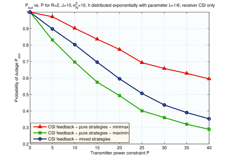
Figure 9: Outage probability vs. transmitter power constraint $\mathcal{P}$ for $M=1$ when $\mathcal{J}=10$, $R=2$, $\sigma_{N}^{2}=10$ and $h$ is distributed exponentially, with parameter $\lambda=1/6$.

As expected, the solution of the of mixed strategies game is better (from the transmitter’s point of view) than the minimax and worse than the maximin solutions of the pure strategies game.

V CSI Available Receiver Only. Jamming Game with Long-Term Power Constraints: Mixed Strategies

In this section we investigate the scenario when the receiver does not feed back any channel state information. Since we have already shown that the problem with long-term power constraints is the more interesting and challenging one, and since the purpose of this section is to offer a comparison with previous results, we further focus only on the scenario of average power constraints and mixed strategies.

Unlike in the corresponding Section V of [1], where all frames were equivalent because of the fast fading channel, in our present scenario each frame is characterized by a particular channel realization. Since this channel realization is not known to either the transmitter or the jammer, they both have to allocate some power over each frame, in a random fashion, such that the transmitter minimizes and the jammer maximizes the probability that the mutual information over the frame is less than the transmission rate $R$. In its most general form, the game can be written as

$$\min_{P_{M}:\mathbf{E}P_{M}\leq\mathcal{P}}\max_{J_{M}:\mathbf{E}J_{M}\leq\mathcal{J}}\mathbf{E}_{P_{M},J_{M}}$$

$$\Bigg{[}\min_{P_{m}:\sum P_{m}\leq MP_{M}}\max_{J_{m}:\sum J_{m}\leq J_{M}}$$

$$Pr\{\sum_{m=0}^{M-1}\log\left(1+\frac{P_{m}h_{m}}{J_{m}+\sigma_{N}^{2}}\right)\leq MR\}\Bigg{]},$$ (97)

where $\mathbf{E}_{P_{M},J_{M}}$ denotes statistical expectation with respect to the probability distribution of $P_{M}$ and $J_{M}$. The form of (V) suggests two levels of power control: a first one which deals with the allocation of power between different frames, and a second one which allocates the powers within each frame.

In solving the game, we start as before with the second level of power control. However, this level requires an exact expression of $Pr\{\sum_{m=0}^{M-1}\log\left(1+\frac{P_{m}h_{m}}{J_{m}+\sigma_{N}^{2}}\right)\leq MR\}$. Note that this probability depends upon the probability distribution of the channel vector $\mathbf{h}$. A practical way of solving the problem is the following.

Denote $S_{m}=\log\left(1+\frac{P_{m}h_{m}}{J_{m}+\sigma_{N}^{2}}\right)$ the random variable (depending on $h_{m}$) which characterizes the instant mutual information over the $m$-th block of the frame. We can write the cumulative distribution function (c.d.f.) of $S_{m}$ as

$$F_{S_{m}}(x)=Pr\{S_{m}\leq x\}=$$

$$=Pr\{h_{m}\leq(e^{x}-1)\frac{J_{m}+\sigma_{N}^{2}}{P_{m}}\}=F_{h}\left((e^{x}-1)\frac{J_{i}+\sigma_{N}^{2}}{P_{i}}\right)$$ (98)

where $F_{h}(x)$ is the c.d.f. of the channel coefficient $h_{m}$ and we assume that the channel coefficients over all the blocks of a frame are independent and identically distributed random variables.

We can now compute the p.d.f. (assuming it exists) of $S_{m}$ as

$$f_{S_{m}}(x)=\frac{dF_{S_{m}}(x)}{dx}=\frac{dF_{h}\left((e^{x}-1)\frac{J_{m}+\sigma_{N}^{2}}{P_{m}}\right)}{dx}.$$ (99)

Finally, our probability can be written as

$$Pr\{\sum_{m=0}^{M-1}\log\left(1+\frac{P_{m}h_{m}}{J_{m}+\sigma_{N}^{2}}\right)\leq MR\}=$$

$$=\left(F_{S_{0}}*f_{S_{1}}*\ldots*f_{S_{M-1}}\right)(MR)$$ (100)

where $*$ denotes regular convolution. Due to the intricate expression of this probability, as well as its dependence on the statistical properties of the channel, we next focus exclusively on the simple case when $M=1$.

Particular case: $M=1$

For $M=1$, we are only concerned with the first level of power control. The game can be written as

$$\min_{P_{M}:\mathbf{E}P_{M}\leq\mathcal{P}}\max_{J_{M}:\mathbf{E}J_{M}\leq\mathcal{J}}$$

$$\mathbf{E}_{P_{M},J_{M}}Pr\{P\leq(c-1)\frac{J_{M}+\sigma_{N}^{2}}{h}\}$$ (101)

or equivalently,

$$\min_{P_{M}:\mathbf{E}P_{M}\leq\mathcal{P}}\max_{J_{M}:\mathbf{E}J_{M}\leq\mathcal{J}}$$

$$\mathbf{E}_{P_{M},J_{M}}Pr\{h\leq(c-1)\frac{J_{M}+\sigma_{N}^{2}}{P_{M}}\}.$$ (102)

In order to provide a good numerical comparison with the results of the previous sections, assume that the channel coefficient $h$ has an exponential probability distribution with parameter $\lambda$. Its cumulative distribution function can thus be written as $F(h)=1-e^{-\lambda h}$, which enables us to write

$$Pr\{h\leq(c-1)\frac{J_{M}+\sigma_{N}^{2}}{P_{M}}\}=$$

$$=1-\exp\left[-\lambda(c-1)\frac{J_{M}+\sigma_{N}^{2}}{P_{M}}\right].$$ (103)

Denote $H(P_{M},J_{M})=1-\exp\left[-\lambda(c-1)\frac{J_{M}+\sigma_{N}^{2}}{P_{M}}\right]$.

By computing the derivatives

$$\frac{dH}{dP_{M}}=$$

$$=-\lambda(c-1)\frac{J_{M}+\sigma_{N}^{2}}{P_{M}^{2}}\exp\left[-\lambda(c-1)\frac{J_{M}+\sigma_{N}^{2}}{P_{M}}\right]<0,$$ (104)

$$\frac{d^{2}H}{dP_{M}^{2}}=$$

$$=\lambda(c-1)\frac{J_{M}+\sigma_{N}^{2}}{P_{M}^{3}}\left[\lambda(c-1)\frac{J_{M}+\sigma_{N}^{2}}{P_{M}}+2\right]$$

$$\exp\left[-\lambda(c-1)\frac{J_{M}+\sigma_{N}^{2}}{P_{M}}\right]>0,$$ (105)

$$\frac{dH}{dJ_{M}}=$$

$$=\lambda(c-1)\frac{1}{P_{M}}\exp\left[-\lambda(c-1)\frac{J_{M}+\sigma_{N}^{2}}{P_{M}}\right]>0,$$ (106)

and

$$\frac{d^{2}H}{dJ_{M}^{2}}=$$

$$=-(\lambda(c-1)\frac{1}{P_{M}})^{2}\exp\left[-\lambda(c-1)\frac{J_{M}+\sigma_{N}^{2}}{P_{M}}\right]<0,$$ (107)

we notice that $H$ is a strictly decreasing, convex function of $P_{M}$ for a fixed $J_{M}$, and a strictly increasing, concave function of $J_{M}$ for a fixed $P_{M}$. Hence, a Nash equilibrium is achieved by uniformly distributing the transmitter’s and jammer’s powers between the frames:

$$\mathbf{E}_{P_{M}:\mathbf{E}P_{M}\leq\mathcal{P}}\left\{1-\exp\left[-\lambda(c-1)\frac{\mathcal{J}+\sigma_{N}^{2}}{P_{M}}\right]\right\}\leq{}$$

$${}\leq 1-\exp\left[-\lambda(c-1)\frac{\mathcal{J}+\sigma_{N}^{2}}{\mathcal{P}}\right]\leq{}$$

$${}\leq\mathbf{E}_{J_{M}:\mathbf{E}J_{M}\leq\mathcal{J}}\left\{1-\exp\left[-\lambda(c-1)\frac{J_{M}+\sigma_{N}^{2}}{\mathcal{P}}\right]\right\}$$ (108)

This saddlepoint is an equilibrium of pure strategies, and hence also an equilibrium of mixed strategies. Note that the existence of such an equilibrium of pure strategies might no longer hold for different probability distributions of $h$, and this would demand a search for purely probabilistic strategies. For example, when the c.d.f. of the channel coefficient $F(h)$ is not concave, then $F((c-1)\frac{J_{M}+\sigma_{N}^{2}}{P_{M}})$ is no longer a concave function of $J_{M}$, and hence the optimal jammer strategy is not deterministic.

Numerical evaluations of the system’s performance under the present scenario are presented in the next subsection.

V-A Numerical results

The probability of outage as a function of the transmitter’s power constraint $\mathcal{P}$ is shown in Figure 10 for $M=1$, and under the assumption that both the transmitter and the jammer distribute their powers uniformly over the frames.

For comparison, the maximin and minimax solutions of the pure strategies game and the mixed strategies Nash equilibrium, all under the scenario that channel state information is fed back by the receiver, are also shown in the figure.

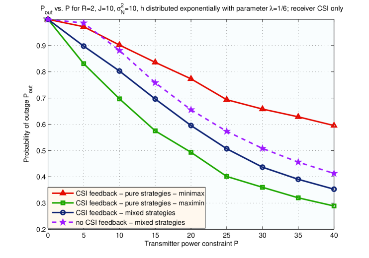
Figure 10: Outage probability vs. transmitter power constraint $\mathcal{P}$ for $M=1$, with and without CSI feedback when $\mathcal{J}=10$, $R=2$, $\sigma_{N}^{2}=10$ and $h$ is distributed exponentially, with parameter $\lambda=1/6$. (Mixed strategies.)

Note that when the receiver does not feed back the CSI, the system performance suffers degradation. Unlike in the fast fading scenario of [1], in the present slow fading scenario the increase in the outage probability is significant. The difference is most visible at low transmitter powers, when not feeding back the channel state information amounts to worse performance than the pessimistic (minimax) scenario with full CSI.

VI Conclusions

We have studied the jamming game over slow fading channels, with the outage probability as objective. Similarly to the fast fading scenario, the game with full CSI and average (or long term) power constraints does not have a Nash equilibrium of pure strategies. Nevertheless, we derived the minimax and maximin solutions of pure strategies, which provide lower and upper bounds on the system performance, respectively.

In addition, we investigated the Nash equilibrium of mixed strategies. Compared to the fast fading scenario [1], the Nash equilibrium for the slow fading, full CSI game is much more involved. The difference comes from the fact that frames are not equivalent. In fact, instead of being characterized by the channel statistics as in [1], the frames are now characterized by different channel realizations. This results in the existence of an additional third level of power control.

We also showed that for parallel slow fading channels, the CSI feedback helps in the battle against jamming, since if the receiver does not feed back the channel state information, the system’s performance suffers a significant degradation. We expect this degradation to decrease as the number of parallel channels $M$ increases, until it becomes marginal for $M\to\infty$ (which can be considered as the case in [1]).

These results, along with our conclusions from the first part of this paper [1], reveal an interesting duality between the ways that different communication models behave with and without jamming. As remarked in [1], under a fast fading channel with jamming, the feedback of channel state information brings little benefits in terms of the overall probability of outage. The same tendency is observed for the fast fading channel without jamming in [14] (although the performance measure therein is the ergodic capacity). However, [10] shows that for a parallel slow fading channel, the CSI feedback is quite important. The improvement of the probability of outage when the channel coefficients are perfectly known to the transmitter is no longer negligible. The results of our present paper demonstrate that even in the presence of a jammer (which can eavesdrop the feedback channel and hence obtain the same CSI as the transmitter), CSI feedback improves the transmission considerably.

Appendix A Short-Term Power Constraints - Proofs of Main Results

A-A Proof of Proposition 1

The proof is an adaptation of the results in Section IV.B of [2], regarding uncorrelated jamming with CSI at the transmitter. The only difference is that in our case, the power constraints and cost function involve short-term, temporal averages, while in [2], they are expressed in terms of statistical averages. Nevertheless, the same techniques can be applied.

The set of all pairs $(P(h),J(h))$ satisfying the power constraints is convex, since the power constraints are linear functions of $P(h)$ and $J(h)$, respectively. Moreover, the cost function

$$I_{M}(\mathbf{h},P(h),J(h))=\frac{1}{M}\sum_{m=0}^{M-1}\log(1+\frac{h_{m}P_{m}}{\sigma_{N}^{2}+J_{m}})$$

is a convex function of $J(h)$ for fixed $P(h)$, and a concave function of $P(h)$ for fixed $J(h)$. These properties imply that there exists at least one saddle point of the game.

Writing the KKT conditions for both optimization problems we get [2]:

$$-\frac{h}{\sigma_{N}^{2}+J(h)+hP(h)}+\lambda-\gamma(h)=0$$ (109)

and

$$-\frac{hP(h)}{(\sigma_{N}^{2}+J(h))(\sigma_{N}^{2}+J(h)+hP(h))}+\nu-\delta(h)=0,$$ (110)

where $\gamma(h)$ and $\delta(h)$ are the complementary slackness variables for $P(h)$ and $J(h)$, respectively.

The three possible cases are [2]: Case 1: $P(h)>0$, $J(h)>0$; Case 2: $P(h)>0$, $J(h)=0$ and Case 3: $P(h)=J(h)=0$.

For Case 1 both complementary slackness variables are $0$, and solving (109) and (110) together we get

$$\frac{\lambda}{\mu}=\frac{J(h)+\sigma_{N}^{2}}{P(h)},$$ (111)

and

$$P(h)=\frac{h}{\lambda(h+\lambda/\mu)},$$ (112)

while for Cases 2 and 3, the solution is plain water-filling [2].

These considerations result in the solutions (15) and (18).

A-B Proof of Theorem 1

This proof follows the one described in the Appendix B of [10]. The probability of outage can be written as:

$$Pr(I_{M}(\mathbf{h},P(h),J(h))<R)=E[\chi_{\{I_{M}(\mathbf{h},P(h),J(h))<R\}}],$$ (113)

where $\chi_{\{\mathscr{A}\}}$ denotes the indicator function of the set $\mathscr{A}$. Replacing the power allocations by the solutions of the game described by (9) and (12), we define

$$\chi^{*}(\mathbf{h})=\chi_{\{I_{M}(\mathbf{h},P^{*}(h),J^{*}(h))<R\}}.$$ (114)

Then the region $\mathcal{U}(R,\mathcal{P},\mathcal{J})$ can be written as:

$$\mathcal{U}(R,\mathcal{P},\mathcal{J})=\{\mathbf{h}\in\mathbb{R}_{+}^{M}:\chi^{*}(\mathbf{h})=0\}.$$ (115)

We next use the fact that the pair $(P^{*}(h),J^{*}(h))$ determines an equilibrium of the game (9), (12). Thus, for any random power allocation $P(h)$ satisfying the power constraint, we can write:

$$\chi^{*}(\mathbf{h})\leq\chi_{\{I_{M}(\mathbf{h},P(h),J^{*}(h))<R\}},\textrm{with probability 1}.$$ (116)

Similarly, for any random $J(h)$, we have

$$\chi^{*}(\mathbf{h})\geq\chi_{\{I_{M}(\mathbf{h},P^{*}(h),J(h))<R\}},\textrm{with probability 1}.$$ (117)

Now pick some arbitrary power allocation functions $P_{a}(h)$ and $J_{a}(h)$, which satisfy the short-term power constraints, and set

$$\widehat{P}(h)=(1-\chi^{*}(\mathbf{h}))P^{*}(h)+\chi^{*}(\mathbf{h})P_{a}(h),$$ (118)

and

$$\widehat{J}(h)=(1-\chi^{*}(\mathbf{h}))J_{a}(h)+\chi^{*}(\mathbf{h})J^{*}(h),$$ (119)

It is easy to see that $1/M\sum_{m=0}^{M-1}\widehat{P}(h_{m})\leq\mathcal{P}$ with probability $1$ , $1/M\sum_{m=0}^{M-1}\widehat{J}(h_{m})\leq\mathcal{J}$ with probability $1$, and moreover that

$$\chi^{*}(\mathbf{h})=\chi_{\{I_{M}(\mathbf{h},\widehat{P}(h),\widehat{J}(h))<R\}}.$$ (120)

Note that transmitter and jammer could pick $P_{a}(h)=0$ and $J_{a}(h)=0$ respectively, but this strategy would not improve their performances (power cannot be saved), since the only power constraints are set over frames.

Now, using (113), (116) and (117), we get:

$$Pr(I_{M}(\mathbf{h},P(h),\widehat{J}(h))<R)\geq{}$$

$${}\geq Pr(I_{M}(\mathbf{h},\widehat{P}(h),\widehat{J}(h))<R)\geq{}$$

$${}\geq Pr(I_{M}(\mathbf{h},\widehat{P}(h),J(h))<R),$$ (121)

which proves the existence of a Nash equilibrium of the original game.

Appendix B Long-Term Power Constraints: Pure Strategies

B-A Proof of Proposition 2

Take Problem 1. Let $(\mathfrak{P}^{*},\mathfrak{J}^{*})=\big{(}(P_{0}^{*},P_{1}^{*},\ldots,P_{M-1}^{*}),(J_{0}^{*},J_{1}^{*},\ldots,J_{M-1}^{*})\big{)}$ be a solution such that $\sum_{m=0}^{M-1}P_{m}^{*}=P_{M,1}$ and $\sum_{m=0}^{M-1}J_{m}^{*}=J_{M,1}$, and assume that $I_{M}(\mathfrak{P}^{*},\mathfrak{J}^{*})>R$. Since $I_{M}$ is a continuous, strictly increasing function of $P_{0}$, without loss of generality, we can find $P_{0}^{\prime}<P_{0}^{*}$ such that $I_{M}((P_{0}^{\prime},P_{1}^{*},\ldots,P_{M-1}^{*}),\mathfrak{J}^{*})=R$.

But then $P_{0}^{\prime}+\sum_{m=1}^{M-1}P_{m}^{*}<MP_{M,1}$, which means that $(\mathfrak{P}^{*},\mathfrak{J}^{*})$ is suboptimal (from the transmitter’s point of view), and hence not a solution.

Therefore, the first constraint $I_{M}\geq R$ has to be satisfied with equality, i.e. $I_{M}=R$.

Now take the solution $(\mathfrak{P}^{*},\mathfrak{J}^{*})$, and assume that $\frac{1}{M}\sum_{m=0}^{M-1}J_{m}^{*}<J_{M}$. Then we can find $J_{0}^{\prime}>J_{0}^{*}$, such that $J_{0}^{\prime}+\sum_{m=1}^{M-1}J_{m}^{*}=MJ_{M}$. In order for the first constraint $I_{M}=R$ to be satisfied, the value and distribution of $P_{M}$ will have to be modified.

We prove next that the value of $P_{M}$ should be increased, which makes the pair $(\mathfrak{P}^{*},\mathfrak{J}^{*})$ suboptimal (from the jammer’s point of view), thus contradicting the hypothesis that it is a solution, and proving that the second constraint should hold with equality.

Assume there is a distribution $\mathfrak{P}^{\prime\prime}=(P_{0}^{\prime\prime},P_{1}^{\prime\prime},\ldots,P_{M-1}^{\prime\prime})$ that minimizes $P_{M}$, under the constraint $I_{M}(\{P_{m}\},(J_{0}^{\prime},J_{1}^{*},\ldots,J_{M-1}^{*}))=R$, such that

$$\sum_{m=0}^{M-1}P_{m}^{\prime\prime}\leq P_{M,1}.$$ (122)

Then, replacing $J_{0}$ by its old value $J_{0}^{*}$, we have that $(\mathfrak{P}^{\prime\prime},\mathfrak{J}^{*})$ is either a second solution of Problem 1 (if (122) is satisfied with equality), or a better choice (if (122) is satisfied with strict inequality). We can readily dismiss the latter case. For the former case, $I_{M}$ is a strictly decreasing function of $J_{0}$, thus $I_{M}(\mathfrak{P}^{\prime\prime},\mathfrak{J}^{*})>R$, which contradicts the first part of this proof. The same arguments work for Problem 2.

B-B Proof of Proposition 3

Proposition 3 is a direct consequence of Theorem 8 in the Appendix II.D of [1]. We restate the theorem here for completeness. For a complete proof, see the first part of this paper [1].

Theorem 6

Take $x,y\in L^{2}[\mathbb{R}]$ and define the order relation $x>y$ if and only if $x(t)>y(t)~{}\forall t\in\mathbb{R}$. Consider the continuous real functions $f(x)$, $g(y)$ and $h(x,y)$ over $L^{2}[\mathbb{R}]$, such that $f$ is a strictly increasing function of $x$, $g$ is a strictly increasing function of $y$, and $h$ is a strictly increasing function of $x$ for fixed $y$ and a strictly decreasing function of $y$ for fixed $x$.

Define the following minimax and maximin problems:

$$\max_{y\geq 0}\left[\min_{x\geq 0}f(x)~{}\textrm{s.t.}~{}h(x,y)\geq H\right]\textrm{s.t.}g(y)\leq G,$$ (123)

$$\max_{x\geq 0}\left[\min_{y\geq 0}g(y)~{}\textrm{s.t.}~{}h(x,y)\leq H\right]\textrm{s.t.}f(x)\leq F,$$ (124)

$$\min_{y\geq 0}\left[\max_{x\geq 0}h(x,y)~{}\textrm{s.t.}~{}f(x)\leq F\right]\textrm{s.t.}g(y)\leq G.$$ (125)

(I) Choose any real values for $G$ and $H$. Take problem (123) under these constraints and let the pair $(x_{1},y_{1})$ denote one of its optimal solutions, yielding a value of the objective function $f(x_{1})=F_{1}$. If we set the value of the corresponding constraints in problems (124) and (125) to $F=F_{1}$, then the values of the objective functions of problems (124) and (125) under their optimal solutions are $g(y)=G$ and $h(x,y)=H$, respectively. Moreover, $(x_{1},y_{1})$ is also an optimal solution of all problems.

(II) Choose any real values for $F$ and $H$. Take problem (124) under these constraints and let the pair $(x_{2},y_{2})$ denote one of its optimal solutions, yielding a value of the objective function $g(y_{2})=G_{2}$. If we set the value of the corresponding constraints in problems (123) and (125) to $G=G_{2}$, then the values of the objective functions of problems (123) and (125) under their optimal solutions are $f(x)=F$ and $h(x,y)=H$, respectively. Moreover, $(x_{2},y_{2})$ is an optimal solution of all problems.

(III) Choose any real values for $F$ and $G$. Take problem (125) under these constraints and let the pair $(x_{3},y_{3})$ denote one of its optimal solutions, yielding a value of the objective function $h(x_{3},y_{3})=H_{3}$. If we set the value of the corresponding constraints in problems (123) and (124) to $H=H_{3}$, then the values of the objective functions of problems (123) and (124) under their optimal solutions are $f(x)=F$ and $g(y)=G$, respectively. Moreover, $(x_{3},y_{3})$ is an optimal solution of all problems.

B-C Proof of Proposition 4

Take Problem 1. By Proposition 3, if there exists $P_{M,1}$ such that solving the game in (9) and (12) with the constraint $\sum_{m=1}^{M-1}P_{m}\leq MP_{M,1}$ yields the objective $I_{M}(\mathbf{h},\{P_{m}\},\{J_{m}\})=R$, then the solution of Problem 1 coincides with the solution of the game in (9) and (12).

We write this solution as in (15) and (18), but we denote $\lambda=1/\eta$ and $\mu=\nu/\eta$:

$$P_{m}^{*}=\left\{\begin{array}[]{ccc}(\lambda-\frac{\sigma_{N}^{2}}{h_{m}})^{+}&\textrm{if}&h_{m}<\frac{\sigma_{N}^{2}}{\lambda-\sigma_{N}^{2}\mu}\\ \mu\frac{\lambda h_{m}}{1+\mu h_{m}}&\textrm{if}&h_{m}\geq\frac{\sigma_{N}^{2}}{\lambda-\sigma_{N}^{2}\mu}\end{array}\right.$$ (128)

$$J_{m}^{*}=\left\{\begin{array}[]{ccc}0&\textrm{if}&h_{m}<\frac{\sigma_{N}^{2}}{\lambda-\sigma_{N}^{2}\mu}\\ \frac{\lambda h_{m}}{1+\mu h_{m}}-\sigma_{N}^{2}&\textrm{if}&h_{m}\geq\frac{\sigma_{N}^{2}}{\lambda-\sigma_{N}^{2}\mu}\end{array}\right.$$ (131)

where $\lambda$ and $\mu$ are constants that can be determined from the constraints $\sum_{m=1}^{M-1}J_{m}=MJ_{M}$ and $\sum_{m=1}^{M-1}I(h_{m},P_{m},J_{m})=MR$.

We shall use the following conventions and denotations:

• Without loss of generality, we shall assume that the blocks in a frame are indexed in increasing order of their channel coefficients. That is, $h_{0}\leq h_{1}\leq\ldots,\leq h_{M-1}$.

• Denote $x_{m}=J_{m}+\sigma_{N}^{2}$ and $x_{m}^{*}=J_{m}^{*}+\sigma_{N}^{2}$. Note that $\frac{x_{0}^{*}}{h_{0}}\geq\frac{x_{1}^{*}}{h_{1}}\geq\ldots,\geq\frac{x_{M-1}^{*}}{h_{M-1}}$.

• Denote by $h_{p}$ the first block on which the transmitter’s power is strictly positive, and by $h_{j}$ the first block on which the jammer’s power is strictly positive. Note that $h_{p}\leq h_{j}$.

Note that

$$P_{m}^{*}=\left[\lambda-\frac{x_{m}^{*}}{h_{m}}\right]_{+}$$ (132)

for all $m\in\{0,1,\ldots,M-1\}$, where $[z]_{+}=\max\{z,0\}$.

Given these and (128) and (131) above, we can write:

$$\frac{\sigma_{N}^{2}}{h_{p}}\leq\lambda<\frac{\sigma_{N}^{2}}{h_{p-1}},$$ (133)

$$\sigma_{N}^{2}\frac{1+\mu h_{j}}{h_{j}}\leq\lambda<\sigma_{N}^{2}\frac{1+\mu(h_{j-1})}{h_{j-1}},$$ (134)

$$MR=\sum_{m=p}^{j-1}\log\left(\frac{\lambda h_{m}}{\sigma_{N}^{2}}\right)+{}$$

$${}-\sum_{m=j}^{M-1}\log\left(\frac{1}{1+\mu h_{m}}\right),$$ (135)

Denote by $Q_{U}[h]$ denotes the index of the smallest channel coefficient in the frame that is larger than $h$. With this notation, we can write

$$p\geq Q_{U}\left[\frac{h_{j-1}}{1+\mu h_{j-1}}\right]$$ (136)

$$h_{p-1}<\frac{h_{j}}{1+\mu h_{j}}$$ (137)

$$\frac{1}{M}\sum_{m=j}^{M-1}\left[\frac{\frac{h_{m}}{1+\mu h_{m}}}{\frac{h_{j}}{1+\mu h_{j}}}-1\right]\leq\frac{J_{M}}{\sigma_{N}^{2}}\leq$$

$$\frac{1}{M}\sum_{m=j}^{M-1}\left[\frac{\frac{h_{m}}{1+\mu h_{m}}}{\frac{h_{j-1}}{1+\mu h_{j-1}}}-1\right],$$ (138)

$$\sum_{m=Q_{U}\left[\frac{h_{j}}{1+\mu h_{j}}\right]}^{j-1}\log\left(h_{m}\frac{1+\mu h_{j}}{h_{j}}\right)-{}$$

$${}-\sum_{m=j}^{M-1}\log\left(\frac{1}{1+\mu h_{m}}\right)\leq MR\leq{}$$

$${}\leq\sum_{m=Q_{U}\left[\frac{h_{j-1}}{1+\mu h_{j-1}}\right]}^{j-1}\log\left(h_{m}\frac{1+\mu(h_{j-1})}{h_{j-1}}\right)-{}$$

$${}-\sum_{j}^{M-1}\log\left(\frac{1}{1+\mu h_{m}}\right),$$ (139)

where (B-C) follows from $J_{M}=\sum_{m=j}^{M-1}\left[\frac{\lambda h_{m}}{1+\mu h_{m}}-\sigma_{N}^{2}\right]$, and the first inequality in (B-C) follows since $h_{p-1}<\frac{h_{j}}{1+\mu h_{j}}$ implies $p\leq Q_{U}\left[\frac{h_{j}}{1+\mu h_{j}}\right]$ because there is no other channel coefficient between $h_{p-1}$ and $h_{p}$.

It is straightforward to show that for fixed $h_{j}$ the left-most and the right-most terms of inequality (B-C) are strictly decreasing functions of $\mu$, while the left-most and the right-most terms of inequality (B-C) are strictly increasing functions of $\mu$.

Note that

$$\sum_{m=j}^{M-1}\left[\frac{\frac{h_{m}}{1+\mu h_{m}}}{\frac{h_{j}}{1+\mu h_{j}}}-1\right]=\sum_{m=j+1}^{M-1}\left[\frac{\frac{h_{m}}{1+\mu h_{m}}}{\frac{h_{j}}{1+\mu h_{j}}}-1\right],$$ (140)

and

$$\sum_{m=Q_{U}\left[\frac{h_{j}}{1+\mu h_{j}}\right]}^{j-1}\log\left(h_{m}\frac{1+\mu h_{j}}{h_{j}}\right)-{}$$

$${}-\sum_{m=j}^{M-1}\log\left(\frac{1}{1+\mu h_{m}}\right)={}$$

$${}=\sum_{m=Q_{U}\left[\frac{h_{j}}{1+\mu h_{j}}\right]}^{j}\log\left(h_{m}\frac{1+\mu h_{j}}{h_{j}}\right)-{}$$

$${}-\sum_{m=j+1}^{M-1}\log\left(\frac{1}{1+\mu h_{m}}\right).$$ (141)

That is, by keeping $\mu$ constant and replacing $h_{j}$ by $h_{j-1}$ in both first terms of (B-C) and (B-C), we get exactly the last terms of (B-C) and (B-C), respectively.

Finally, we take a contradictory approach. Suppose there exist two different pairs $(h_{j1},\mu_{1})$ and $(h_{j2},\mu_{2})$ that satisfy both (B-C) and (B-C) and assume, without loss of generality that $h_{j1}<h_{j2}$. Then, in order for $(h_{j2},\mu_{2})$ to satisfy (B-C) we need $\mu_{2}>\mu_{1}$, while in order for $(h_{j2},\mu_{2})$ to satisfy (B-C) we need $\mu_{<}\mu_{1}$. Thus $h_{j}$ is unique. Note however that the relations above do not guarantee the uniqueness of $\mu$.

For the optimal $h_{j}$, the constraint $\sum_{m=1}^{M-1}J_{m}=MJ_{M}$ translates to

$$\sum_{m=j}^{M-1}\frac{\lambda h_{m}}{1+\mu h_{m}}=MJ_{M}+(M-j)\sigma_{N}^{2}.$$ (142)

while the constraint $I_{M}(\mathbf{h},\{P_{m}\},\{J_{m}\})=R$ is already given in (B-C). The left hand side of (142) is a strictly increasing function of $\lambda$ for fixed $\mu$ and a strictly decreasing function of $\mu$ for fixed $\lambda$, while being equal to a constant.

Again, for a contradictory approach, suppose there exist two different pairs of $(\mu_{1},\lambda_{1})$ and $(\mu_{2},\lambda_{2})$ that can generate different solutions. If we assume, without loss of generality that $\mu_{1}>\mu_{2}$, then, in order for (142) to be satisfied by both pairs, we need $\lambda_{1}>\lambda_{2}$. But this can only mean that under $(\mu_{2},\lambda_{2})$ the transmitter allocates non-zero power to more channel coefficients than under $(\mu_{1},\lambda_{1})$. This remark simply says that the index $p$ at which the transmitter starts transmitting is a decreasing function of $\lambda$, and can easily be verified by (132).

Looking now at (B-C), we observe that its right hand side is a strictly increasing function of $\lambda$ for fixed $\mu$ and a strictly increasing function of $\mu$ for fixed $\lambda$, while being equal to a constant. In other words, if (B-C) is satisfied by the pair $(\mu_{1},\lambda_{1})$, then it cannot also be satisfied by $(\mu_{2},\lambda_{2})$. Thus, the pair $(\lambda,\mu)$ that satisfies both (B-C) and (142) is also unique. But once $h_{j}$, $\lambda$ and $\mu$ are given, $h^{p}$ is uniquely determined. Therefore there cannot exist more than one solution to Problem1.

Similar arguments can be applied to show that the solution of Problem2 is unique.

B-D Proof of Proposition 5

Since the solution is unique, it follows that $\mathscr{P}_{M}(J_{M})$ is a strictly increasing function. By closely inspecting the form of the solution in (128) and (131), it is straightforward to see that if $J_{M}\to\infty$, then $J_{m}\to\infty$ for all $m\in\{0,1,\ldots,M-1\}$. If the required $P_{M}$ were finite, this would imply $I_{M}\to 0$, which violates the power constraints of Problem 1.

For Problem 1 we prove that the resulting $\mathscr{P}_{M}(J_{M})$ function is continuous and concave in several steps. We first show in Lemma 1 that the optimal jammer strategy $\{x_{m}^{*}\}_{m=0}^{M-1}$ is a continuous function of the given jamming power $J_{M}$. Lemma 2 proves that $P_{M}(\{x_{m}\})$ is continuous and has continuous first order derivatives. This implies that $P_{M}(J_{M})$ is in fact continuous and has a continuous first order derivative. Finally, Lemma 3 shows that for any fixed $h_{p}$ and $h_{j}$ the function $P_{M}(J_{M})$ is concave.

Lemma 1

The optimal jammer power allocation $\{x_{m}^{*}\}_{m=0}^{M-1}$ within a frame is a continuous increasing function of the given jamming power $J_{M}$ invested over that frame.

Proof:

It is clear that $x_{m}^{*}$ is continuous and increasing as a function of $J_{M}$ if $h_{p}$ and $h_{j}$ are fixed. At any point where either $h_{p}$ or $h_{j}$ change as a result of a change in $J_{M}$, the optimal jamming strategy $\{x_{m}^{*}\}_{m=0}^{M-1}$ maintains continuity as a result of the uniqueness of the solution (Proposition 4). ∎

Lemma 2

Both $P_{M}(\{x_{m}\})$ and the derivatives $\frac{dP_{M}}{dx_{m}}$ are continuous functions of $\{x_{m}\}_{m=0}^{M-1}$.

Proof:

Consider any two points $\mathfrak{X}_{1}=(x_{1,m})_{m=0}^{M-1}$ and $\mathfrak{X}_{2}=(x_{2,m})_{m=0}^{M-1}$ and any trajectory $\mathfrak{T}$ that connects them.

For a given vector $\mathfrak{X}=(x_{m})_{m=0}^{M-1}$, the required transmitter power is

$$P_{M}=\frac{M-p}{M}\left(\frac{c}{\left(\prod_{m=p}^{M-1}h_{m}\right)}\right)^{\frac{1}{M}}\left(\prod_{m=p}^{M-1}x_{m}\right)^{\frac{1}{M}}-{}$$

$${}-\frac{1}{M}\sum_{m=p}^{M-1}\frac{x_{m}}{h_{m}}.$$ (143)

Note that $p$ depends upon the choice of $\mathfrak{X}$. For fixed $p$, the continuity and differentiability of $P_{M}(\mathfrak{X})$ are obvious. Thus, it suffices to show that these properties also hold in a point of $\mathfrak{T}$ where $p$ changes.

If we can show continuity and differentiability when $p$ is decreased by $1$, then larger variations of $p$ can be treated as multiple changes by $1$, and continuity still holds.

Recall the assumption that the channel coefficients are always indexed in decreasing order of the quantities $\frac{x_{m}}{h_{m}}$. Let $\mathfrak{X}_{k}=(x_{k,m})_{m=0}^{M-1}$ be a point of $\mathfrak{T}$ where the transmitter decreases the index of the block over which it starts to transmit from $p_{k}$ to $p_{k}-1$, and denote by $\mathfrak{T_{1}}$ the part of the trajectory $\mathfrak{T}$ that is between $\mathfrak{X}_{1}$ and $\mathfrak{X}_{k}$, and $\mathfrak{T_{2}}=\mathfrak{T}\setminus\mathfrak{T_{1}}$.

Since $P_{p_{k}-1}=0$, we know that $\lambda$ does not change in this point, since

$$\frac{1}{M}\sum_{m=p}^{M-1}\left[\lambda-\frac{x_{m}}{h_{m}}\right]=\frac{1}{M}\sum_{m=p-1}^{M-1}\left[\lambda-\frac{x_{m}}{h_{m}}\right]=P_{M}.$$ (144)

Define the “left” and “right” limits $P_{M}(\mathfrak{X}_{k}-)$ and $P_{M}(\mathfrak{X}_{k}+)$ as:

$$P_{M}(\mathfrak{X}_{k}-)=\lim_{\begin{subarray}{c}\mathfrak{X}\to\mathfrak{X}^{k}\\ \mathfrak{X}\in\mathfrak{T_{1}}\end{subarray}}P_{M}(\mathfrak{X}),$$ (145)

$$P_{M}(\mathfrak{X}_{k}+)=\lim_{\begin{subarray}{c}\mathfrak{X}\to\mathfrak{X}^{k}\\ \mathfrak{X}\in\mathfrak{T_{2}}\end{subarray}}P_{M}(\mathfrak{X}).$$ (146)

Since $\mathbb{R}_{+}^{M}$ is Hausdorff [15], there exists a small enough neighborhood $\mathfrak{U}\subset\mathbb{R}_{+}^{M}$ of $\mathfrak{X}_{k}$, such that $p(\mathfrak{X})=p_{k}$ to the “left” and $p(\mathfrak{X})=p_{k}-1$ to the “right” of $\mathfrak{X}_{k}$ on $\mathfrak{U}$. We can now write:

$$P_{M}(\mathfrak{X}_{k}+)={}$$

$${}=\lambda\frac{M-p_{k}+1}{M}-\frac{1}{M}\sum_{m=p_{k}-1}^{M-1}\frac{x_{k,m}}{h_{m}}={}$$

$${}=\lambda\frac{M-p_{k}}{M}-\frac{1}{M}\sum_{m=p_{k}}^{M-1}\frac{x_{k,m}}{h_{m}}+{}$$

$${}+\frac{1}{M}(\lambda-\frac{x_{k,p_{k}-1}}{h_{p_{k}-1}})=P_{M}(\mathfrak{X}_{k}-),$$ (147)

where the last equality follows because $\lambda=\frac{x_{k,p_{k}-1}}{h_{p_{k}-1}}$. This proves continuity.

Similar arguments can be used to show the continuity of the derivatives

$$\frac{dP_{M}}{dx_{n}}=\frac{1}{M}\left(\frac{\lambda}{x_{n}}-\frac{1}{h_{n}}\right)$$ (148)

in $\mathfrak{X}_{k}$ (note that $\frac{\lambda}{x_{k,p_{k}-1}}=\frac{1}{h_{p_{k}-1}}$).

Therefore, $P_{M}(\mathfrak{X})$ is continuous and has first-order derivatives that are continuous along any trajectory $\mathfrak{T}$ between any two points $\mathfrak{X}_{1}$ and $\mathfrak{X}_{2}$. ∎

Finally, for the last part of our proof:

Lemma 3

For fixed $p$ and $j$, the function $P_{M}(J_{M})$ is concave.

Proof:

We can write

$$MJ_{M}+(M-j)\sigma_{N}^{2}=\Bigg{[}c\prod_{m=p}^{j-1}\left(\frac{\sigma_{N}^{2}}{h_{m}}\right)^{\frac{1}{M}}\cdot$$

$$\cdot\prod_{m=j}^{M-1}\left(\frac{1}{1+\mu h_{m}}\right)^{\frac{1}{M}}\Bigg{]}^{\frac{M}{j-p}}\sum_{m=j}^{M-1}\frac{h_{m}}{1+\mu h_{m}},$$ (149)

and denote

$$g(\mu)=\prod_{m=j}^{M-1}\left(\frac{1}{1+\mu h_{m}}\right)^{\frac{1}{j-p}}\sum_{m=j}^{M-1}\frac{h_{m}}{1+\mu h_{m}}$$ (150)

Note that for fixed $p$ and $j$, $J_{M}$ is a linear function of $g$.

A similar relation can be found for the required transmitter power $P_{M}$:

$$MP_{M}+\frac{1}{M}\sum_{m=p}^{j-1}\frac{\sigma_{N}^{2}}{h_{m}}=\Bigg{[}c\prod_{m=p}^{j-1}\left(\frac{\sigma_{N}^{2}}{h_{m}}\right)^{\frac{1}{M}}\cdot$$

$$\cdot\prod_{m=j}^{M-1}\left(\frac{1}{1+\mu h_{m}}\right)^{\frac{1}{M}}\Bigg{]}^{\frac{M}{j-p}}\cdot{}$$

$${}\cdot\left[\frac{M-p}{M}-\frac{1}{M}\sum_{m=j}^{M-1}\frac{1}{1+\mu h_{m}}\right].$$ (151)

Denote

$$f(\mu)=\prod_{m=j}^{M-1}\left(\frac{1}{1+\mu h_{m}}\right)^{\frac{1}{j-p}}\cdot{}$$

$${}\cdot\left[(M-p)-\sum_{m=j}^{M-1}\frac{1}{1+\mu h_{m}}\right]$$ (152)

and note that for fixed $p$ and $j$, $P_{M}$ is a linear function of $f$.

It suffices to show that $f(g)$ is concave. For this purpose, the derivative $\frac{df}{dg}=\frac{df}{d\mu}(\frac{d\mu}{dg})^{-1}$ should be a decreasing function of $g$, and hence an increasing function of $\mu$.

Computing the derivatives from (B-D) and (B-D) we get:

$$\frac{df}{dg}=\frac{\frac{df}{d\mu}}{\frac{dg}{d\mu}}={}$$

$${}=\frac{\frac{1}{j-p}\left((M-p)-\sum_{m=j}^{M-1}\frac{1}{1+\mu h_{m}}\right)-\frac{\sum_{m=j}^{M-1}\frac{h_{m}}{(1+\mu h_{m})^{2}}}{\sum_{m=j}^{M-1}\frac{h_{m}}{1+\mu h_{m}}}}{\frac{1}{j-p}\sum_{m=j}^{M-1}\frac{h_{m}}{(1+\mu h_{m})^{2}}+\frac{\sum_{m=j}^{M-1}\frac{h_{m}^{2}}{(1+\mu h_{m})^{2}}}{\sum_{m=j}^{M-1}\frac{h_{m}}{1+\mu h_{m}}}}$$ (153)

Arguments similar to those in [1] apply in proving that above the derivative increases with $\mu$. Looking at the right hand side of (B-D) (the “large fraction”), we notice that the first term in the numerator increases with $\mu$. For the second term in the numerator, it is clear that as $\mu$ increases, its numerator decreases faster than its denominator. This implies that the whole numerator of the “large fraction” is an increasing function of $\mu$. Similarly, the first term in the denominator is clearly a decreasing function of $\mu$. The only thing left is the second term of the denominator. It is straightforward to show that its derivative with respect to $\mu$ can be written as

$$\frac{d}{d\mu}\frac{\sum_{m=j}^{M-1}\frac{h_{m}^{2}}{(1+\mu h_{m})^{2}}}{\sum_{m=j}^{M-1}\frac{h_{m}}{1+\mu h_{m}}}=\frac{1}{\left[\sum_{m=j}^{M-1}\frac{h_{m}}{1+\mu h_{m}}\right]^{2}}\cdot$$

$$\cdot\Bigg{\{}\left[\sum_{m=j}^{M-1}\frac{h_{m}^{2}}{(1+\mu h_{m})^{2}}\right]^{2}-\sum_{m=j}^{M-1}\frac{h_{m}^{3}}{(1+\mu h_{m})^{3}}\cdot$$

$$\cdot\sum_{m=j}^{M-1}\frac{h_{m}}{(1+\mu h_{m})}\Bigg{\}}$$ (154)

If we consider the fact that for any two real numbers $a$ and $b$ we have

$$(a^{2}+b^{2})^{2}-(a+b)(a^{3}+b^{3})=-ab(a-b)^{2}$$ (155)

and the summations in (B-D) are positive, it is easy to see that the second term of the denominator of the “large fraction” is decreasing with $\mu$. Hence overall the derivative in (B-D) increases with $\mu$.

∎

Appendix C Long Term Power Constraints: Mixed Strategies

C-A Proof of Theorem 4

Denote the solution of the game in (9) and (12), where the jammer is constrained to $\frac{1}{M}\sum_{m=1}^{M-1}J_{m}\leq J_{M}(p_{M})$ and the transmitter is constrained to $\frac{1}{M}\sum_{m=1}^{M-1}P_{m}\leq p_{M}$ by $(\{P_{m,1}\},\{J_{m,1}\})$, and the solution of the game in (9) and (12), where the transmitter is constrained to $\frac{1}{M}\sum_{m=1}^{M-1}P_{m}\leq P_{M}(j_{M})$ and the jammer is constrained to $\frac{1}{M}\sum_{m=1}^{M-1}J_{m}\leq j_{M}$ by $(\{P_{m,2}\},\{J_{m,2}\})$.

Denote the solution of the game in (9) and (12), where the jammer is constrained to $\frac{1}{M}\sum_{m=1}^{M-1}J_{m}\leq j_{M}$ and the transmitter is constrained to $\frac{1}{M}\sum_{m=1}^{M-1}P_{m}\leq p_{M}$ by $(\{P_{m,0}\},\{J_{m,0}\})$..

By the Proposition 2, we must have $I_{M}(\{P_{m,1}\},\{J_{m,1}\})=R$ and $I_{M}(\{P_{m,2}\},\{J_{m,2}\})=R$, where $I_{M}(\{P_{m}\},\{J_{m}\})=\frac{1}{M}\sum_{m=0}^{M-1}\log(1+\frac{P_{m}h_{m}}{J_{m}+\sigma_{N}^{2}})$.

We will show that (i) even if the jammer’s power $j_{M}$ is different from $J_{M}(p_{M})$, the transmitter’s strategy is still optimal; (ii) even if the transmitter’s power $p_{M}$ is different from $P_{M}(j_{M})$, the jammer’s strategy is still optimal.

Assume the transmitter plays the strategy given by $\{P_{m,1}\}$.

If $j_{M}=J_{M}(p_{M})$, it is clear that the optimal solution for both transmitter and jammer is the solution of the game in (9) and (12), where the jammer is constrained to $\frac{1}{M}\sum_{m=1}^{M-1}J_{m}\leq j_{M}$ and the transmitter is constrained to $\frac{1}{M}\sum_{m=1}^{M-1}P_{m}\leq p_{M}$. In this case, it is as if each player knows the other player’s power constraint.

If $j_{M}<J_{M}(p_{M})$, then by Lemma 1 we have that $J_{m,0}<J_{m,1}~{}\forall m$. Since $I_{M}(\{P_{m}\},\{J_{m}\})$ is a strictly decreasing function of $\{J_{m}\}$ (under the order relation defined in the Appendix III of [1]), this implies that $I_{M}(\{P_{m,1}\},\{J_{m,1}\})>R$. Note that $\{J_{m,0}\}$ is the jammer’s strategy when the jammer knows the transmitter’s power constraint $p_{M}$. Thus we have shown that when the transmitter plays $\{P_{m,1}\}$ and $j_{M}<J_{M}(p_{M})$, the jammer cannot induce outage over the frame even if it knew the value of $p_{M}$.

Assume that the jammer plays the strategy given by $\{J_{m,2}\}$. A similar argument shows that if $p_{M}<P_{M}(j_{M})$, or equivalently $j_{M}>J_{M}(p_{M})$, the transmitter cannot achieve reliable communication over the frame even if it knew the exact value of $j_{M}$.

This shows that $(\{P_{m,1}\},\{J_{m,2}\})$ is a Bayes equilibrium [12] for the game with incomplete information describing the power allocation within a frame.

C-B Proof of Proposition 9

Take any solution $\{P_{M}(h)^{*}\},\{J_{M}(h)^{*}\}$ of the KKT conditions and denote by $P_{out}^{*}$ the outage probability obtained under these strategies. By maintaining $\{J_{M}(h)^{*}\}$ constant and changing $\{P_{M}(h)^{*}\}$, the resulting probability of outage can only be greater than or equal to $P_{out}^{*}$, since the original $\{P_{M}(h)^{*}\}$ is the solution of a minimization problem with convex cost function and linear constraints.

Similarly, by maintaining $\{P_{M}(h)^{*}\}$ constant and changing $\{J_{M}(h)^{*}\}$, the resulting probability of outage can only be less than or equal to $P_{out}^{*}$, since the original $\{J_{M}(h)^{*}\}$ is the solution of a maximization problem with concave cost function and linear constraints.

These arguments imply that $\{P_{M}(h)^{*}\},\{J_{M}(h)^{*}\}$ is a Nash equilibrium of the game.

References

- [1] G. T. Amariucai and S. Wei, “Jamming in fixed-rate wireless systems with power constraints - part I: Fast fading channels,” submitted to IEEE Trans. Inform. Theory. Available on arXiv 2008, Aug. 2008.
- [2] S. Shafiee and S. Ulukus, “Correlated jamming in multiple access channels,” Conference on Information Sciences and Systems, March 2005.
- [3] T. Basar, “The Gaussian test channel with an intelligent jammer,” IEEE Trans. Inform. Theory, vol. 29, pp. 152–157, Jan. 1983.
- [4] T. Basar and Y.-W. WU, “A complete characterization of minimax and maximin encoder-decoder policies for communication channels with incomplete statistical description,” IEEE Trans. Inform. Theory, vol. 31, pp. 482–489, July 1985.
- [5] M. Medard, “Capacity of correlated jamming channels,” Allerton Annual Conf. on Comm., Control and Computing, 1997.
- [6] B. Hughes and P. Narayan, “Gaussian arbitrarily varying channels,” IEEE Trans. Inform. Theory, vol. 33, pp. 267–284, March 1987.
- [7] R. K. Mallik, R. A. Scholtz, and G. P. Papavassilopuolos, “Analysis of an On-Off jamming situation as a dynamic game,” IEEE Trans. Commun., vol. 48, pp. 1360–1373, Aug. 2000.
- [8] E. Altman, K. Avrachenkov, and A. Garnaev, “A jamming game in wireless networks with transmission cost,” Proceedings of Net-Coop, Avignon, France, June 2007.
- [9] D. Tse and P. Viswanath, Fundamentals of Wireless Communication. Cambridge University Press, 2005.
- [10] G. Caire, G. Taricco, and E. Biglieri, “Optimum power control over fading channels,” IEEE Trans. Inform. Theory, vol. 45, pp. 1468–1489, July 1999.
- [11] S. N. Diggavi and T. Cover, “The worst additive noise under a covariance constraint,” IEEE Trans. Inform. Theory, vol. 47, pp. 3072–3081, Nov. 2001.
- [12] R. B. Meyerson, Game Theory (Analysis of Conflict). Harvard University Press, 1997.
- [13] J.-P. Aubin, Optima and Equilibria. Springer-Verlag, 1993.
- [14] A. J. Goldsmith and P. P. Varaiya, “Capacity of fading channels with channel state information,” IEEE Trans. Inform. Theory, vol. 43, pp. 1986–1992, Nov. 1997.
- [15] J. R. Munkres, Topology. Prentice-Hall, 2004.