Entanglement control in one-dimensional $s=\frac{1}{2}$ random XY spin chain

Abstract

The entanglement in one-dimensional random XY spin systems where the impurities of exchange couplings and the external magnetic fields are considered as random variables is investigated by solving the different spin-spin correlation functions and the average magnetization per spin. The entanglement dynamics near particular locations of the system is also studied when the exchange couplings (or the external magnetic fields) satisfy three different distributions(the Gaussian distribution, double-Gaussian distribution, and bimodal distribution). We find that the entanglement can be controlled by varying the strength of external magnetic field and the different distributions of impurities. Moreover, the entanglement of some nearest-neighboring qubits can be increased for certain parameter values of the three different distributions.

I Introduction

Entanglement not only has the interesting properties of quantum mechanics but also is very important in the quantum information processing (QIP), such as quantum teleportation^[1], dense coding^[2], quantum secret sharing^[3], quantum computation^[4] and some cryptographic protocols^[5]. In order to realize the quantum information process, a great effort has been made to study and characterize the entanglement in cavity QED^[6-7] and solid state systems. A typical example is the spin chains that can describe interaction of qubits not only in solid physical systems but also in many other systems such as quantum dots^[8], electronic spins^[9], and optical lattices^[10]. Therefore, there have been conducted numerous studies on Ising model^[11] and all kinds of Heisenberg XY XXZ XYZ models^[12-15].
Impurities often exist in solid systems and play an important part in condensed matter physics. As a candidate of QIP, a solid system with impurity is also one of our important study objects. In the previous researches, the effect of impurity on the quantum entanglement has been studied in a three-spin system ^[16-17] and a large spin systems under zero temperature^[18]. However, in these studies, only single impurity has been studied.
Recently, Huang et al^[19-20] have demonstrated that for a class of one-dimensional magnetic systems entanglement can be controlled and tuned by varying the anisotropy parameter in the XY Hamiltonian and by introducing impurities into the systems. However, in Ref.(19), only the impurity and the external magnetic fields in a Gaussian form are considered and the value of the width of the distribution is fixed. In Ref.(20), the strength of the impurity is located at two sites. For the pure case, Osterloh et al^[21] examined the entanglement between two spins at position i and j in the spin chains. Owing to its importance, in this paper we study the entanglement dynamics near particular locations of one-dimensional $s=\frac{1}{2}$ random XY spin system when the exchange couplings (or external magnetic fields) satisfy three different distributions(the Gaussian distribution, double-Gaussian distribution, and bimodal distribution), to our knowledge, which have not been reported yet. The present study in simple examples can help us to understand the behaviour of the entanglement in one-dimensional random XY spin systems for the different distributions. More importantly, we will demonstrate that one can control or manipulate the entanglement in spin system with the help of the exchange couplings and the external magnetic fields.

II Solution of the XY model

We consider a physical Heisenberg XY model of N spin-$\frac{1}{2}$ particles interacting with their nearest neighbours. In the presence of impurities, the one-dimensional Hamiltonian is given by ^[19]

$$H= - \frac{1+\gamma}{2}\sum_{i=1}^{N}J_{i,i+1}\sigma_{i}^{x}\sigma_{i+1}^{x}-\frac{1-\gamma}{2}$$ (1)

$$\times \sum_{i=1}^{N}J_{i,i+1}\sigma_{i}^{y}\sigma_{i+1}^{y}-\sum_{i=1}^{N}h_{i}\sigma_{i}^{z}$$

where $J_{i,i+1}$ is the exchange interaction between sites i and i+1, $h_{i}$ is the strength of the external magnetic field on site i, $\sigma^{x,y,z}$ are the Pauli matrices, $\gamma$ is the degree of anisotropy and N is the number of sites. The periodic boundary conditions satisfy $\sigma_{N+1}^{x}=\sigma_{1}^{x},\sigma_{N+1}^{y}=\sigma_{1}^{y},\sigma_{N+1}^{z}=\sigma_{1}^{z}$.
Now we define the raising and lowing operators $a_{i}^{+}$,$a_{i}^{-}$ and introduce Fermi operators^[22] $c_{j}^{+}$ and $c_{j}$, and they are expressed as follows:

$$a_{i}^{+}=\frac{1}{2}(\sigma_{i}^{x}+i\sigma_{i}^{y})=c_{i}^{+}\exp(i\pi\sum_{j=1}^{i-1}c_{j}^{+}c_{j}),$$ (2)

$$a_{i}^{-}=\frac{1}{2}(\sigma_{i}^{x}-i\sigma_{i}^{y})=\exp(-i\pi\sum_{j=1}^{i-1}c_{j}^{+}c_{j})c_{i}.$$ (3)

so that, the Hamiltonian has the following form

$$H= - \sum_{i=1}^{N}J_{i,i+1}[(c_{i}^{+}c_{i+1}+\gamma c_{i}^{+}c_{i+1}^{+})+h.c]$$ (4)

$$- 2\sum_{i=1}^{N}h_{i}(c_{i}^{+}c_{i}-\frac{1}{2})$$

In the present paper, the exchange interaction has the form $J_{i,i+1}=J(1+\alpha_{i,i+1})$, where $\alpha$ introduces the impurity in the double-Gaussian form with peaks at $\frac{N+1}{2}$ with strength $\zeta_{1}$ and at $\frac{N-1}{2}$ with strength $\zeta_{2}$,

$$\alpha_{i,i+1} = P\times\zeta_{1}\exp\{-\epsilon(i-\frac{N+1}{2})\}$$ (5)

$$+ (1-P)\times\zeta_{2}\exp\{-\epsilon(i-\frac{N-1}{2})\}$$

The external magnetic field takes the form $h_{i}=h(1+\beta_{i})$, where

$$\beta_{i} = P\times\xi_{1}\exp\{-\epsilon(i-\frac{N+1}{2})\}$$ (6)

$$+ (1-P)\times\xi_{2}\exp\{-\epsilon(i-\frac{N-1}{2})\}$$

When $\alpha=\beta=0$, the above reduces to a pure case; when $P=1$, the above reduces to the case in Ref.(19). By introducing the dimensionless parameter $\lambda=J/(2h)$, the symmetrical matrix A and the antisymmetrical B, the Hamiltonian becomes

$$H=\sum_{i,j=1}^{N}[c_{i}^{+}A_{i,j}c_{j}+\frac{1}{2}(c_{i}^{+}B_{i,j}c_{j}^{+}+h.c)]$$ (7)

The above Hamiltonian can be diagonalized by making linear transformation of the fermionic operators $\eta_{k}=\sum_{i=1}^{N}g_{ki}c_{i}+h_{ki}c_{i}^{+},\eta_{k}^{+}=\sum_{i=1}^{N}g_{ki}c_{i}^{+}+h_{ki}c_{i},$ and then the Hamiltonian becomes

$$H=\sum_{k=1}^{N}\Lambda_{k}\eta_{k}^{+}\eta_{k}+const,$$ (8)

and two coupled matrix equations satisfy $\phi_{k}(A-B)=\Lambda_{k}\psi_{k},\psi_{k}(A+B)=\Lambda_{k}\phi_{k},$ where the components of the two column vectors $\phi_{ki},\psi_{ki}$ are given by $\phi_{ki}=g_{ki}+h_{ki},\psi_{ki}=g_{ki}-h_{ki}.$ Finally, the ground state of the system $\left|\psi_{0}\right\rangle$ can be written as $\eta_{k}\left|\psi_{0}\right\rangle=0$.

III Spin-spin correlation functions

Before we dicuss the entanglement, we should have a brief review of spin-spin correlation functions. The spin-spin correlation functions for ground state and the average magnetization per spin are respectively defined as ^[22]

$S_{lm}^{x}=\frac{1}{4}\left\langle\psi_{0}\left|\sigma_{l}^{x}\sigma_{m}^{x}\right|\psi_{0}\right\rangle,S_{lm}^{y}=\frac{1}{4}\left\langle\psi_{0}\left|\sigma_{l}^{y}\sigma_{m}^{y}\right|\psi_{0}\right\rangle,$

$S_{lm}^{z}=\frac{1}{4}\left\langle\psi_{0}\left|\sigma_{l}^{z}\sigma_{m}^{z}\right|\psi_{0}\right\rangle,M_{i}^{z}=\frac{1}{2}\left\langle\psi_{0}\left|\sigma_{i}^{z}\right|\psi_{0}\right\rangle.$

These correlation functions are given as expectation values of products of fermion operators. Using Wicks theorem^[23], these expressions can be rewritten as

$S_{lm}^{x}=\frac{1}{4}\left(\begin{array}[]{cccc}G_{l,l+1}&G_{l,l+2}&\cdots&G_{l,m}\\ \vdots&\vdots&\ddots&\vdots\\ G_{m-1,l+1}&G_{m-1,l+1}&\cdots&G_{m-1,m}\end{array}\right)$,

$S_{lm}^{y}=\frac{1}{4}\left(\begin{array}[]{cccc}G_{l+1,l}&G_{l+1,l+1}&\cdots&G_{l+1,m-1}\\ \vdots&\vdots&\ddots&\vdots\\ G_{m,l}&G_{m,l+1}&\cdots&G_{m,m-1}\end{array}\right)$

$S_{lm}^{z}=\frac{1}{4}(G_{l,l}G_{m,m}-G_{m,l}G_{l,m}),M_{i}^{z}=\frac{1}{2}G_{i,i}$

where $G_{i,j}=-\sum_{k}^{N}\psi_{ki}\phi_{kj}$

IV Entanglement of nearest-neighbouring qubits

In this part, we give the expression of the concurrence that quantifies the amount of the entanglement between two qubits. For a system described by the density matrix$\rho$, the concurrence C is^[24]

$$C(\rho)=\max(0,\lambda_{1}-\lambda_{2}-\lambda_{3}-\lambda_{4})$$ (9)

Here $\lambda_{1}$, $\lambda_{2}$, $\lambda_{3}$, $\lambda_{4}$ are the eigenvalues (of them $\lambda_{1}$ is the largest) of the spin-flipped density operator R, which is defined by $R=\sqrt{\sqrt{\rho}\tilde{\rho}\sqrt{\rho}}$ , where $\tilde{\rho}=(\sigma_{y}\otimes\sigma_{y})\rho^{\ast}(\sigma_{y}\otimes\sigma_{y})$, $\tilde{\rho}$ denoting the complex conjugate of $\rho$ with $\sigma_{y}$ being the usual Pauli matrix. The values of concurrence C ranges from zero to one; when $C=0$, the two qubits are in an unentangled state, when $C=1$, the two qubits are in an maximally entangled state.
Using the operator expansion for the density matrix and the symmetries of the Hamiltonian^[25], in the basis states $\{\left|\uparrow\uparrow\right\rangle,\left|\uparrow\downarrow\right\rangle,\left|\downarrow\uparrow\right\rangle,\left|\downarrow\downarrow\right\rangle\}$, $\rho$ has the general form

$\rho=\left(\begin{array}[]{cccc}\rho_{1,1}&0&0&\rho_{1,4}\\ 0&\rho_{2,2}&\rho_{2,3}&0\\ 0&\rho_{3,2}&\rho_{3,3}&0\\ \rho_{4,1}&0&0&\rho_{4,4}\end{array}\right),$
with
$\lambda_{a}=\sqrt{\rho_{1,1}\rho_{4,4}}+\left|\rho_{1,4}\right|,\lambda_{b}=\sqrt{\rho_{2,2}\rho_{3,3}}+\left|\rho_{2,3}\right|,$
$\lambda_{c}=\sqrt{\rho_{1,1}\rho_{4,4}}-\left|\rho_{1,4}\right|,\lambda_{d}=\sqrt{\rho_{2,2}\rho_{3,3}}-\left|\rho_{2,3}\right|,$

We can express all the matrix elements in the density matrix in terms of different spin-spin correlation functions:

$\rho_{1,1}=\frac{1}{2}M_{l}^{z}+\frac{1}{2}M_{m}^{z}+S_{lm}^{z}+\frac{1}{4},$

$\rho_{2,2}=\frac{1}{2}M_{l}^{z}-\frac{1}{2}M_{m}^{z}-S_{lm}^{z}+\frac{1}{4},$

$\rho_{3,3}=\frac{1}{2}M_{m}^{z}-\frac{1}{2}M_{l}^{z}-S_{lm}^{z}+\frac{1}{4},$

$\rho_{4,4}=-\frac{1}{2}M_{l}^{z}-\frac{1}{2}M_{m}^{z}+S_{lm}^{z}+\frac{1}{4},$

$\rho_{2,3}=S_{lm}^{x}+S_{lm}^{y},$

$\rho_{1,4}=S_{lm}^{x}-S_{lm}^{y},$

V Results and discussions

In this paper, we focus our discussions on the transverse Ising model with $\gamma=1$. Our goal is to examine the dynamics of entanglement in the varying of the exchange couplings and the external magnetic fields. First, we examine the change of the entanglement for the nearest neighbouring concurrence C(i,i+1)for different values of the impurity as the parameter $\lambda$ varies. We consider two kinds of nearest neighbouring concurrences near particular locations of the system. Figure 1 depicts the nearest neighbouring concurrence C(49,50) as a function of the reduced coupling constant $\lambda$ at different values of the impurity $\zeta$ for different distributions with the system size N =101 and the anisotropy parameter $\gamma=1$. Figure 1(a) shows the change of concurrence C(49,50) as a function of different values $\lambda$ with $p=1$, i.e the Gaussian distribution. We can see that the concurrence increases and arrives at a maximum close to the critical point $\lambda_{c}$, and it is close to zero above $\lambda_{c}$. As $\zeta$ increases the concurrence tends to increase faster and the $\lambda_{m}$, where concurrence approaches a maximum, shift to left very rapidly. This is consistent with the result in Ref. [19](Fig.1). In Fig.1(b), 1(c), and 1(d), we give the curves for the concurrence against the width of the double-Gaussian distribution. The two Gaussian distributions have equal probability with $p=0.5$, and the central positions are at $\frac{N+1}{2}$ and $\frac{N-1}{2}$. Here one of the double-Gaussian distribution is fixed with $\zeta_{1}=0.5$. We first investigate the situation when the width of the double-Gaussian distribution $\epsilon$ is 0.1, A similar behaviour can be seen in Fig.1(b), only the changed width becomes narrow. As $\epsilon$ increases, the concurrence increases slowly and the peak value decreases, which is shown in Fig.1(c). As is well known, bimodal distribution is a particular case of the double-Gaussian distribution, that is to say, the double-Gaussian distribution is converted into bimodal distribution as $\epsilon$ increases. In Fig.1(d), $\epsilon=10$. The numerical calculations show that concurrence decreases with the increase of $\zeta_{2}$, which indicates that the behaviours are very different from the former cases.
In Fig.2, we show the results of the nearest neighbouring concurrence between the sites 49 and 50, as a function of the parameter $\lambda$ for different strengths of the external magnetic field $\xi$. The effect of the external magnetic field $\xi$ in the Gaussian distribution is also shown in Fig.2(a). However, different from the effect of the exchange couplings, the concurrence increases slowly and tends to move to infinity by increasing the value of the parameter $\xi$. This is also consistent with the result in Ref. [19](Fig.1). A similar behaviour can be seen in Fig.2(b) for the double-Gaussian distribution, however, with $\xi=1$ and $\xi=10$, it is interesting to find that the entanglement peak between the nearest neighbours increases to a value larger than that in Fig.2(a). As $\xi$ increases, the concurrence increases rapidly below $\lambda_{c}$, while the concurrence increases slowly above $\lambda_{c}$. A comparison between the dash curve and the dash dotted curve in Fig.2(d) shows that the concurrence increases rapidly and tends to move to infinity by increasing the value of the parameter $\xi_{2}$, which is different from the results obtained from the Gaussian distribution and double-Gaussian distribution. That is to say, the strong $\xi_{2}$ is helpful to keep the better entanglement for the bimodal distribution.
Up to now we have examined the nearest neighbouring concurrence C(49,50) with different Gaussian distributions for purities and strengths of magnetic field. It is interesting to study the effect of the different Gaussian distributions on the concurrence for the rest of the sites in the chain. For the Ising model, a similar analysis can be carried out for the nearest neighbouring concurrence C(50,51),the concurrence is located at the centre of the double-Gaussian distribution. This is demonstrated in Figs.3 and 4 by the evolutions of the concurrence. Figure 3 corresponds to the case in which the exchange couplings are varying, and the peak of the maximal entanglement becomes larger than that in Fig.1. It is the different distributions that lead to considerable different evolutions of the entanglement, hence the entanglement is rather sensitive to any small change in the exchange interaction for the bimodal distribution. As shown in Eq.(5), for the bimodal distribution, the strengths of impurity are mostly located at two sites($\alpha_{49,50},\alpha_{50,51}$). The nearest neighbouring concurrence increases with the increasing of $\zeta_{2}$, so that by adjusting $\zeta_{2}$ one can obtain a strong entanglement. The results that we have obtained here are also consistent with those in Ref. [20](Fig.4). Figure 4 corresponds to the case in which the external magnetic field is varying, the entanglement between nearest neighbours tends to be reduced in the presence of the external magnetic field for the double-Gaussian distribution and the bimodal distribution, while the entanglement between 49 and 50 increases as shown in Fig.2. The numerical calculations also show that as the parameter $\lambda$ increases from 0 to 4, similar behaviours to those in Figs.2(c) and 2(d) are shown in Figs.4(c) and 4(d).
From the above analysis, it is clear that the three different distributions(the Gaussian distribution, double-Gaussian distribution, and bimodal distribution) have a notable influence on the nearest neighbouring concurrence. As for the case $\gamma\neq 1$(XY model) or the next nearest neighbouring concurrence, we will present further reports in the future.

VI conclusion

The entanglements near particular locations in a one-dimensional $s=\frac{1}{2}$ random XY spin system have been investigated. Through analyzing the exchange couplings (or external magnetic fields) of three different distributions(the Gaussian distribution, double-Gaussian distribution, and bimodal distribution), we have shown that the entanglement can be controlled and enhanced by varying the strengths of the magnetic field and the impurity distribution in the system. The nearest neighbouring concurrence exhibits some interesting phenomena. For a certain distribution, concurrence C(49,50) decreases with the increase of $\zeta$, while concurrence C(50,51) increases. Different behaviours in the varying of the external magnetic field can occur close to and above the critical point. The different distributions play an important role in enhancing the entanglement.

Figure 1: The nearest neighbouring concurrence C(49,50) as a function of the reduced coupling constant $\lambda$ at different values of impurity $\zeta$ for different distributions, with the system size N =101 and the anisotropy parameter $\gamma=1$.

Figure 2: The nearest neighbouring concurrence C(49,50) as a function of the reduced coupling constant $\lambda$ different strengths of the external magnetic field $\xi$, with the system size N =101 and the anisotropy parameter $\gamma=1$.

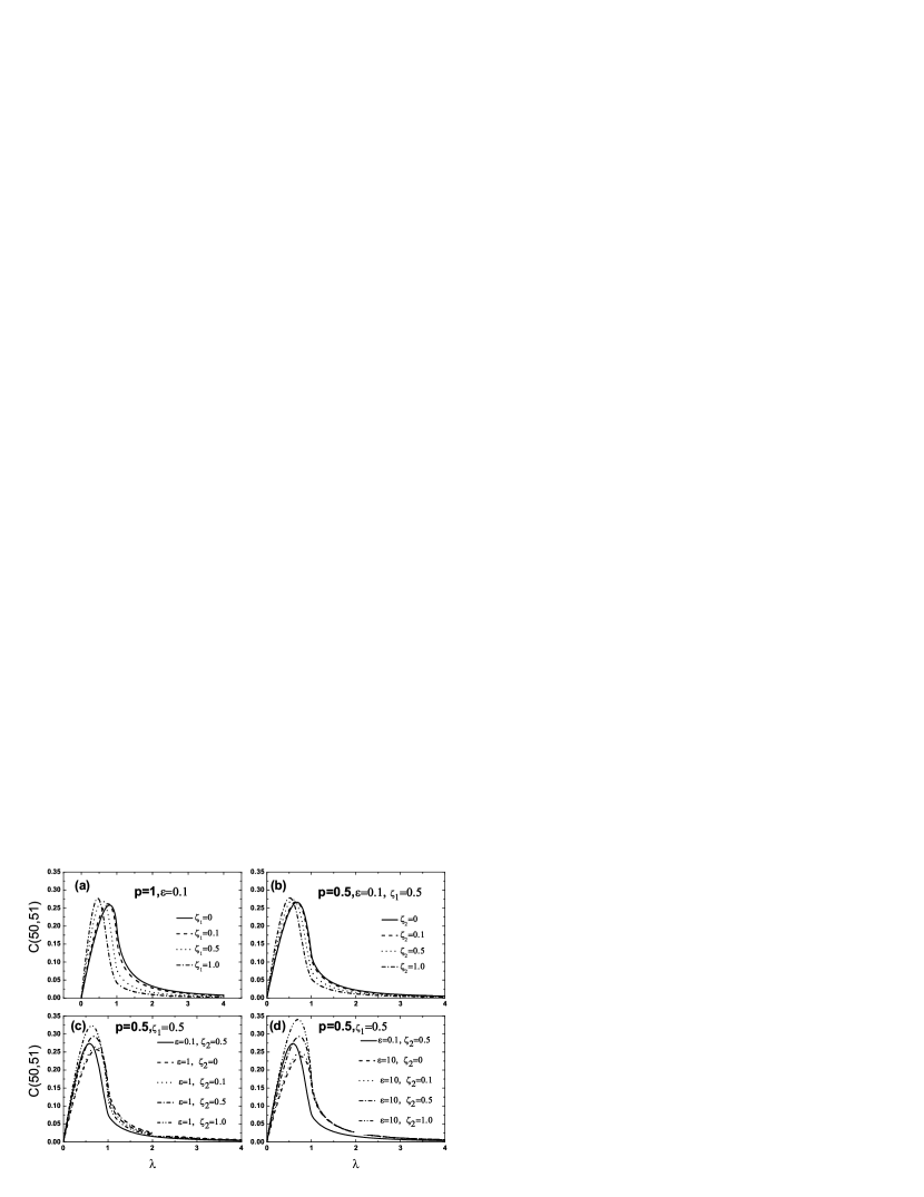
Figure 3: The nearest neighbouring concurrence C(50,51) as a function of the reduced coupling constant $\lambda$ at different values of impurity $\zeta$ for different distributions, with the system size N =101 and the anisotropy parameter $\gamma=1$.

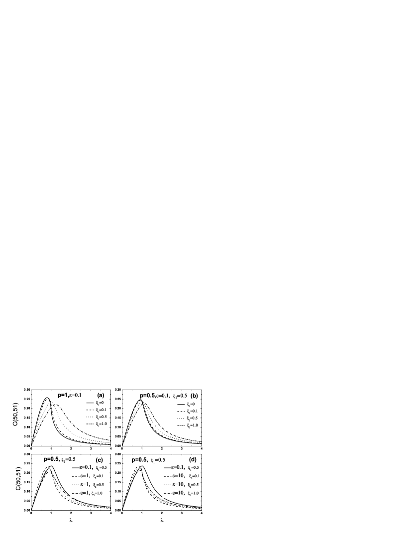
Figure 4: The nearest neighbouring concurrence C(50,51) as a function of the reduced coupling constant $\lambda$ different strengths of the external magnetic field $\xi$, with the system size N =101 and the anisotropy parameter $\gamma=1$.

References

-
(1)
Bennett C H, Brassard G, Cr peau C, Jozsa R, Peres A, and Wootters W K, 1993 Phys. Rev. Lett. 70 1895.
Shan C J, Man Z X, Xia Y J, Liu T K. 2007 Int. J. Quantum Information, 5 359. - (2) Cheng W W, Huang Y X, Liu T K and Li H, 2007 Chin. Phys. 16 38.
- (3) Shan C J, Man Z X, Xia Y J, Liu T K. 2007 Int. J. Quantum Information, 5 335.
- (4) Grover L 1998 Phys. Rev. Lett. 80 4329.
-
(5)
Ma J, Zhang G Y, Rong Y W and Tan L Y 2006 Acta. Phys. Sin. 55 24.
Man Z X, Xia Y J, 2007 Chin. Phys. 16 1197. - (6) Shan C J, Xia Y J 2006 Acta. Phys. Sin. 55 1585.
-
(7)
Liu T K, 2006 Chin. Phys. 15 0542.
Guo D J, Shan C J, Xia Y J 2007 Acta. Phys. Sin. 56 2139. - (8) Loss D, Divincenzo D P,1998 Phys. Rev. A 57 120.
- (9) Kane B E, 1998 Nature(London) 393 133.
- (10) Sorensen A, Molmer K, 1999 Phys. Rev. Lett. 82 4556.
- (11) Wu Y, Machta J, 2005 Phys. Rev. Lett. 95 137208.
- (12) Wang X G 2001 Phys. Rev. A 64 012313.
- (13) Zhang G F and Li S S, 2005 Phys. Rev. A 72 034302.
- (14) Asoudeh M and Karimipour V, 2005 Phys. Rev. A 71 022308.
- (15) Zhou L, Song H S, Guo Y Q, and Li C, 2003 Phys. Rev. A 68 024301.
- (16) Fu H C,Solomon A I, Wang X G, 2002 J. Phys. A 35 4293. Li S B, Xu J B, 2005 Phys. Lett. A 334 109.
- (17) Cheng W W, Huang Y X, Liu T K and Li H, 2007 Physica E 39 150.
- (18) Xin R, Song Z, Sun C P, 2005 Phys. Lett. A 342 30.
- (19) Huang Z, Osenda O, Kais S, 2004 Phys. Lett. A 322 137.
- (20) Osenda O, Huang Z, Kais S, 2003 Phys. Rev. A 67 062321.
- (21) Osterloh A, Amico L, Falci G, and Fazio R, 2002 Nature(London) 416 608.
- (22) Lieb E, Schultz T, Mattis D, 1961 Ann. Phys. 60 407.
- (23) Wick G C, 1950 Phys. Rev. 80 268.
- (24) Wooters W K, 1998 Phys. Rev. Lett. 80 2245.
- (25) Osborne T J, Nielsen M A, 2002 Phys. Rev. A 66 032110.