An X-ray photometry system I: Chandra ACIS

Abstract

We present a system of X-ray photometry for the Chandra satellite. X-ray photometry can be a powerful tool to obtain flux estimates, hardness ratios, and colors unbiased by assumptions about spectral shape and independent of temporal and spatial changes in instrument characteristics. The system we have developed relies on our knowledge of effective area and the energy-to-channel conversion to construct filters similar to photometric filters in the optical bandpass. We show that the filters are well behaved functions of energy and that this X-ray photometric system is able to reconstruct fluxes to within about 20%, without color corrections, for non-pathological spectra. Even in the worst cases it is better than 50%. Our method also treats errors in a consistent manner, both statistical as well as systematic.

1. Introduction

Photometry is one of the most widely used, relatively simple, tools used in describing and categorizing astronomical objects. Standardization by Johnson & Morgan (1953) and subsequent additions in the optical and infrared (see e.g. Bessell (2005)) have allowed comparisons between measurements by different telescopes and instruments without bias. Important applications of optical photometry include stellar classifications (see e.g. Johnson & Morgan (1953)), galaxy redshifts (Puschell et al., 1981), and the discovery of the most distant quasars in the SDSS (Fan et al., 1999). In particular photometry is important for sources too faint to extract detailed spectra, i.e. most sources, given the almost universal increase of source numbers to faint fluxes.

Although optical astronomy is a much older discipline than X-ray astronomy, optical photometry was established only about 20 years before the beginning of X-ray astronomy in the 1960s. Given the enormous success of optical photometry it seems obvious to use it as a precedent and try to duplicate its success in other wavebands beyond UV and infrared. The X-ray band can be defined as reaching from about 0.1 keV to a few hundred keV, spanning almost 4 decades of frequency – although most work concentrates on the 0.2–20 keV band – compared with 2 octaves in the optical. Moreover, an important difference between optical and X-ray is the typically low number of photons in X-ray astronomy. The X-ray range is photon starved such that sources with a few hundred counts are considered bright in X-rays. This limitation increases the importance of broad-band photometry in the X-ray band.

While X-ray astronomy has used relative, mission-specific photometry for most of its existence, there is, as yet, no standard X-ray photometric system. The usefulness of an X-ray photometric system is evident already from the use of these somewhat idiosyncratic energy bands. The bands used in the past have been chosen for specific purposes, e.g. to use color–color diagrams to diagnose X-ray binary spectral states (White & Marshall, 1984; Hasinger & van der Klis, 1989) where, in the latter, the energy bands are different for each source. Even so, the resulting color–color diagrams have immensely increased our knowledge of X-ray binary spectral/accretion states (e.g. Prestwich et al., 2003; Gierliński & Newton, 2006). Thus a standard X-ray photometric system is highly desirable in X-ray astronomy in order to cross-compare observations of the hundreds of thousands of sources being cataloged by XMM (Watson, 2007), Chandra (Fabbiano et al., 2007), and other missions. Even within a given mission different types of CCDs (XMM) or changes in operating temperature, gain or contamination (Chandra ) mean that simple count rates cannot be used.

However, there have been complicating factors in establishing photometric energy bands beyond individual observations. One cause of this lack of standardization is that the energy ranges covered by different X-ray satellites and instruments differ widely. For example, RXTE/PCA, GINGA and EXOSAT bands have practically no overlap with ROSAT bands; and ASCA, XMM and Chandra bands are somewhere in the middle. Fig. 1 shows a selection of energy bands used by different authors for different X-ray satellites. Most X-ray missions with focusing optics cover the energy range from $\sim$0.1 keV to 10 keV.

Another reason for the lack of a standard photometric system is that in X-rays there are no bright constant point sources in the way that stars can be used for calibration like in the optical.

But the most fundamental cause for the lack of an X-ray photometric system has been the limited spectral resolving power (R$=$E/$\Delta E\sim$1) of proportional counters, which were used in X-ray astronomy from the earliest days through to ROSAT and RXTE. A resolution of R$\sim$1 allows no clean separation of energy bands, and different spectra with similar flux will give widely different flux estimates in any chosen band. In optical terms, the “color correction” is very large. However, with the introduction of X-ray CCDs in ASCA (Burke et al., 1993) this limitation has largely gone away. X-ray CCDs have R$>$10, so comparable to the R$\sim$6 of broad band optical photometry. It seems thus timely to consider the introduction of an X-ray photometric system. Therefore we have investigated how good a photometric system can be created for Chandra ACIS observations and, by extension, for all other X-ray CCDs. We report the encouraging results in this paper.

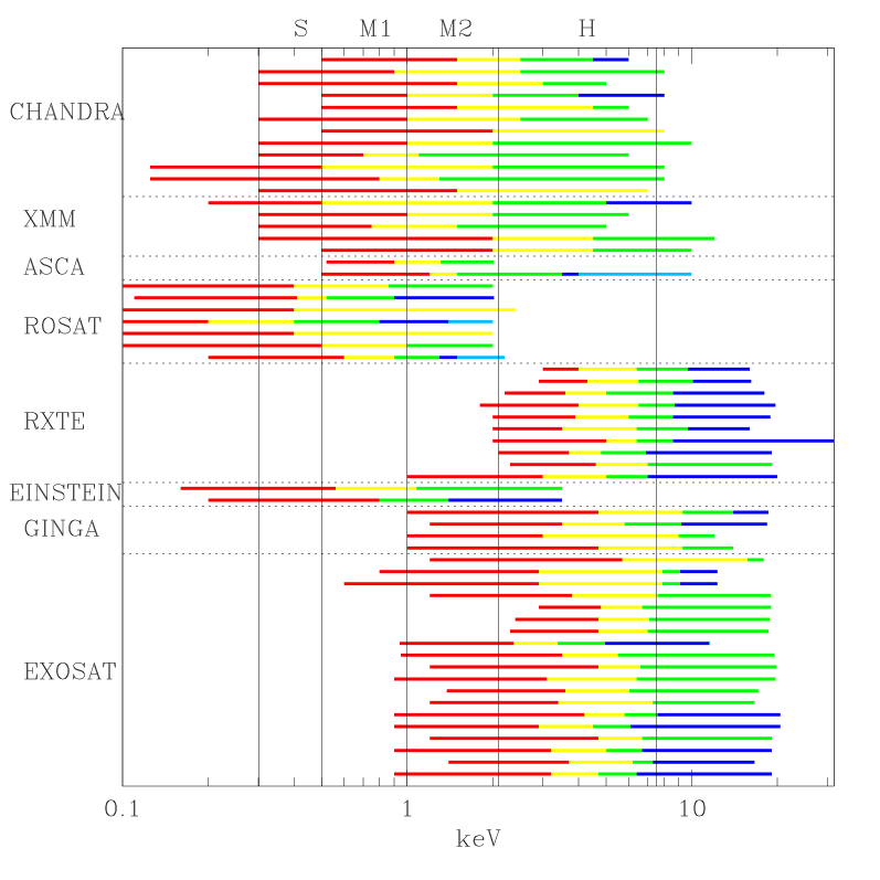
Figure 1.— Energy bands used in various publications for X-ray satellites. The different energy bands for different satellites are due to energy coverage of the instruments. The colors represent the width of the soft/medium/hard bands used in the corresponding papers. A table of energy bands and references are given in the on-line version of the paper.

2. Measurements with Chandra ACIS

The ACIS (Advanced CCD Imaging Spectrometer) instrument is one of the two detectors on Chandra . ACIS is arranged as an array of 10 1024 by 1024 pixel CCDs, one as a two by two array (ACIS-I), and one as a 1 by six array (ACIS-S). The instrument allows simultaneous high resolution imaging and moderate resolution spectroscopy. Two CCDs on ACIS-S are back-illuminated (ACIS-S1 and ACIS-S3), the rest is front-illuminated.

2.1. Energy bands

The black vertical lines in the Fig. 1 are the energy bands we have chosen. They are roughly an octave wide, though the hard band is somewhat wider.

Table 1Standard photometric bands for Chandra 

S	M1	M2	H
soft	medium-soft	medium-hard	hard
0.3–0.5 keV	0.5–1.0 keV	1.0–2.1 keV	2.1–7.5 keV

Because of the similarity of the XMM and Chandra energy ranges wes. will use these bands as a starting point. Most publications use similar bands as can be seen in Fig. 1.

The low energy bound is chosen to be 0.3 keV because the steepness of the ACIS effective area curve for $E<0.3$ keV leads to large dependencies on spectral shape and, secondly, the effective area and photon energy-to-channel conversion for the S-3 chip are not well calibrated below 0.23 keV (P. Plucinksy, priv. comm.). The iridium edge at $\sim$2.1 keV defines the separation between the second medium and hard band. Note that other X-ray mirrors are coated with other high Z elements (e.g. Au, Pt) but these have edges at similar energies (2.3 keV and 2.13 keV, respectively). The high energy boundary is defined by the rapidly rising ACIS background and falling effective area at energies above $\sim$7.5 keV (Chapter 6.16 in CXC (2008)).

The exact location of the boundaries will not strongly affect the analysis of source colors, except for pathological spectral shapes or strong lines at or close to boundaries. For Chandra a much stronger effect, at least in the soft(er) band(s), is the build up of contaminating material on the front of the ACIS, which reduces the effective area significantly compared to the case of no contamination (see 2.2 and Plucinsky et al. (2003); Marshall et al. (2004)).

The number and boundaries of energy bands are of course not immutable, optical photometry also has a variety of more or less different bands for different scientific purposes. For example narrow band filters at neutral or hydrogen-like iron lines or silicon lines can be of interest. Our program to compute correction factors for the count to flux conversion is not limited to the above mentioned energy bands. However, the use of a common standard system across missions is highly desirable as explained in Sec.1.

2.2. ACIS ARF

The ARF (Ancillary Response File) describes the effective area of a telescope at a given energy. All effects related to the probability of detecting a photon with the telescope and detector (quantum efficiency, blockage, mirror area, vignetting) are combined in the ARF. In an ideal system the effective area would be independent of energy. However, the shape of the effective area curve of X-ray telescopes varies far more than for optical telescopes, with variations of factors of a few, even across the octave-wide energy bands used here. Optical telescopes also cover a much smaller logarithmic range of photon energies.

For the back-illuminated (BI) ACIS chips of Chandra , there is significant time variation in the effective area at low energies. Due to resublimation of material on the chips, sensitivity at low energies, up to 0.6 keV, decreased by a factor of $\sim$30 since the beginning of the mission. The sensitivity of the front-illuminated (FI) chips also suffers from accumulation of material but the reduction of low energy effective area is not as pronounced as the area is already quite small for these chips (Plucinsky et al., 2003). This is shown in Fig. 2.

Figure 2.— Effective are curves for the front-illuminated ACIS-I3 chip (top) and the back-illuminated ACIS-S3 chip (bottom) at the aimpoints for the years 1999 to 2008. Years are shown in different lines styles: dotted–1999, dashed–2000, to solid 2008. Years 2004–2007 are not shown because they are almost identical to the 2008 curve. The vertical dotted lines delimit the energy bands.

For more details about changes in the Chandra ARF see Schwartz et al. (2000); Zhao et al. (2004).

2.3. ACIS RMF

The RMF (Redistribution Matrix File) is a matrix that redistributes incident photon energies $E$ (raw energy channels) to PHA or PI channels or observed energy $E^{\prime}$. Neglecting the effective area the observed spectrum in a channel $Sp(E^{\prime})$ is related to the true spectrum at a given energy $E$ by the convolution of incident spectrum with RMF:

$$Sp(E^{\prime}) = Sp(E)\otimes RMF(E^{\prime},E)$$ (1)

$$= \int_{0}^{\infty}Sp(E)\,RMF(E^{\prime},E)\,dE$$

For Chandra the RMF matrix is not symmetric. RMFs for the aimpoints of the main FI and BI chips are shown in Fig. 3. The incident photon energies are binned from 0.1 keV to 11 keV in 10 eV steps. Thus for FI chips there are 1090 raw energy channels; for BI chips there are only 1078 raw channels because these chips are not calibrated below 0.23 keV. The PHA/PI channel number is chosen to be 1024 for both kinds of chips. The values in a row, corresponding to a single raw channel or real photon energy, correspond to the probability of a photon with a given energy being detected in a given PHA/PI channel.

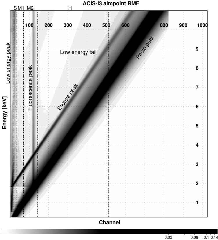
Figure 3.— Response matrices for ACIS-I3 (top) and ACIS-S3 (bottom) at the aimpoint. Grey-scale is logarithmic. Numbers on the right are energy in units of keV, numbers at the top are PHA/PI channel numbers. The vertical dash-dotted lines delimit the energy bands.

The energy to channel conversion is ideally a one to one correlation. But the CCD has a finite energy resolution ($\Delta E\approx 40-170$ eV, depending on energy, location and CCD type). This is larger than the PHA/PI channel width ($\sim$15 eV). Moreover, due to instrumental effects (escape peak, fluorescence peak low energy peak and tail, etc.) a photon of a given energy has a finite probability of being detected in channels corresponding to a lower energy. This is comparable to “red leak” in optical filters.

Taking a slice of the RMF for a given energy (7.5 keV in Fig. 4) results in an approximately Gaussian shaped curve for the main photo peak, containing $\sim$95% of the total, with the FWHM of the main peak contributing about 76% of the total. At around channel 20 there is the so called low energy peak, with an amplitude of about 3 orders of magnitude less than the main peak, that contains about 0.1% of the total. If the photon energy is high enough, i.e. above the Si K edge, there is a secondary peak, the Si fluorescence peak, centered on channel 119 (1.73 keV). The maximum of this secondary peak is about 2-3 orders of magnitude smaller than the main peak. This peak also contains about 0.1% of the total. For photon energies above $\sim$2 keV there is a third peak, the Si escape peak, with an amplitude two orders of magnitude smaller than the main peak. It contributes about 0.6%. It follows about 100 channels behind the main photo peak. Starting at lower energies from the main peak and between the other peaks there is a low energy tail at a level about 3-4 orders of magnitude below the main peak. This tail contains $\sim$4.3% with the biggest contribution, $\sim$3%, in between the Si escape peak and the photopeak. The numbers are almost identical for the two kinds of chips. All these features, peaks and tail, are due to detector effects. In particular, the low energy tail and peak depend on the location at which an X-ray photon interacts with the material of the CCD and produces an electron cloud. An electron cloud from an X-ray photon interaction completely within the gate insulator of the CCD chip produces the low energy peak. Electron clouds that extend partly into the actual detector material, the depleted silicon, contribute to the low energy tail. Finally, the main photo peak is made up of X-ray photon interactions completely within the depleted silicon. The Si fluorescence peak is produced by X-rays exciting Si K shell electrons in the detector material. The escape peak is produced by fluorescence photons that leave the Si substrate or interact away at another location with the detector. Fig. 4 shows a slice of the RMF for a photon of 7.5 keV for the FI ACIS-I3 chip (solid line) and for the BI ACIS-S3 chip (dotted line).

Figure 4.— Slice of the response matrices in PHA space for a photon of energy 7.5 keV. ACIS-I3 (FI) is the solid line and ACIS-S3 (BI) is the dotted line. Both curves are for the aimpoint. The photopeak is the primary signal; the other features are reduced by some two orders of magnitude or more (see text). The broader photopeak for ACIS-I3 results from the larger distance of the aimpoint to the readout compared to ACIS-S3.

For calibration purposes all Chandra ACIS chips are divided into tiles of rectangular form and three different sizes: ACIS-S3 (BI) has a tile size of of 32$\times$32 pixels, ACIS-S1 (BI) has 64$\times$64 pixels, and all the FI chips have 32$\times$256 pixels. This amounts to 2304 tiles over all chips, and thus, in principle 2304 possibly different RMFs. A schematic of the tiling is shown in Fig. 12 in the Appendix.

The main variation among the ACIS RMFs is the widening of the main Gaussian peaks with increasing distance from the readout for the FI chips, i.e. the energy resolution decreases the further a source is from the readout due to charge transfer inefficiency. The energy resolution changes from a FWHM of $\sim$4 channels ($\sim$60 eV) at 1 keV at the readout to $\sim$9 channels ($\sim$130 eV) at the opposite side of the chips. For BI chips spatial variation of the energy resolution has a more complicated shape, but the variation is not as strong as for FI chips. At 1 keV the FWHM changes from 6.3 channels at the readout to 7.4 channels at the opposite side of the chip.

For more details about the Chandra RMFs see Prigozhin et al. (1998); Bautz et al. (1999).

2.4. Photometric bands

The equivalent of filter shapes for the energy bands in Table 1 can be obtained by the convolution of the effective area (ARF) with the RMF PI channels over each energy band. The filter bands constructed for the aimpoints of ACIS-I3 and ACIS-S3 for 1999 and 2007 are shown in Fig. 5. The units are in cm². The four bands have quite different normalizations. The soft band, like the U band in the optical, has the smallest area. The medium-hard and hard bands are quite symmetric and have sharp edges to their main response, as is desirable. The soft and first medium filters have peaks biased towards the high energy ends of their bands. This is the result of the strong energy dependence of the effective area. The low energy leak is quite small. The leakage between energy bands is only in the few per cent range, and moreover can be corrected quite easily, see below.

Figure 5.— X-ray filters for the passbands defined in Sec. 2.1 (dotted vertical lines). Filters are constructed for the aimpoints of ACIS-I3 for 1999 and 2007 (top) and ACIS-S3 for the same years (bottom). Dashed curves refer to 1999, solid curves to 2007.

The X-ray filters have a well defined spatial (from RMF) and temporal (from ARF) dependence. The spatial dependence is related to energy resolution, whereas the main temporal effect is decreasing sensitivity due to accumulation of material on the CCDs.

Except for the hard band, there is a strong effect due to the increased absorption on the CCD between year 1999 and 2007. The increasing energy resolution towards the readout leads to a decreasing overlap between the filter bands. However, the energy resolution of Chandra is generally sufficiently good that this is a small effect ($\sim$3%) even at the opposite chip end from the readout.

These Chandra X-ray filters differ from optical filters in that they have an area normalization given by the ARF, but they are comparable in basic shape. Fig. 6 shows a comparison between the X-ray Chandra filters at the aimpoint of ACIS-S3 in 2008 (in keV) and SDSS ugri filters for zero airmass (in eV). Based on the fractional width of the filters, the X-ray filters are only a factor of 2-4 wider than the SDSS filters. Their variation of the peak sensitivity is about the same.

Figure 6.— Bottom: Filters for the Chandra X-ray photometry system, i.e. combination of ARF and RMF. Abscissa in keV (log scale). Top: SDSS ugri filters for 0 airmass. Abscissa in eV (log scale). The variation of peak transmission among the X-ray filters is comparable to the variation among the optical filters, with the exception of the softest X-ray band. Measured as $\Delta E/E$ the X-ray bands are only a factor of few broader than the optical bands. Note that the width of the four optical filters covers about 3 eV, whereas the four X-ray filters cover about 7000 eV.

Due to the effects described in Sec. 2.3 and illustrated in Fig. 4 each filter contributes somewhat to its adjacent filters and to all lower energy filters. Thus the filter areas are described with a $n\times n$ matrix where $n$ is the number of filters. Since no photon can be detected at higher energies than its own (plus energy resolution effects) the upper right elements of this matrix are zero. This ignores pileup effects in which two photons are detected as one at the sum of the individual photon energies. As an illustration we give the area matrix at the ACIS-S3 aimpoint for 2008:

$$A=\left(\begin{array}[]{cccc}18.7&2.1&0.0&0.0\\ 4.8&241.1&11.9&0.0\\ 1.2&13.4&998.0&9.9\\ 2.1&6.3&30.2&2376.2\end{array}\right)$$ (6)

The units for the elements are in keV cm².

3. Spectral Models

X-ray sources can be separated in various categories, starting with the distinction between point sources and extended sources. The definition of point source is obviously a question of angular resolution, e.g. we know that in X-ray binaries, which are point-like even with Chandra , there are sometimes various regions contributing to X-ray emission. However, given the excellent angular resolution of Chandra (0.3” FWHM at the aimpoint), we consider that a point source for Chandra will be a point source in 15–20 years as well. The approach of photometry is of limited usefulness for extended sources, i.e. plasmas, since a definition of regions is somewhat arbitrary and interpreting photometric differences among regions of one source would require plasma diagnostics that are beyond the scope of this work. Since plasmas are also present in ”point sources”, e.g. extragalactic SNRs, a model is nevertheless included in the following.

To make the photometry system useful for as large a part of the community as possible, it is necessary to study and characterize the accuracy of the photometry for a wide variety of commonly encountered spectral models. Moreover, one of the motivations for a photometric system in X-rays is to not make assumptions about spectral models. However, the conversion of counts, effective area, and exposure time to a flux estimate requires some knowledge of the behavior of spectra. We thus start by taking common spectral models and define a wide range of interest for their parameters. In effect this wide ranging combination of spectral shapes and parameters represents our ignorance of the true spectral shape/parameters of a given source.

Table 2Spectral models and parameter ranges used to estimate photometric accuracy

Component	Parameter	Range	Step size
Absorption	NHa	$10^{20}$–$10^{24}$	0.2 in log
Power law	$\Gamma$	-1.0–4.0	0.2
Black Body	kTb	0.1–2.0	0.2
Bremsstrahlung	kTb	0.5–6.0	0.3
Opt. thin plasma	kTb	0.1–5.0	0.3
	abundancec	0.1–1.0	0.1
Gaussian Line	Energiesb	0.8, 1.3, 1.85, 6.4	n/a
	Line widthsb	0.1, 0.5, 1.0	n/a

^a – units in cm^-2
b – units in keV
^b – units in solar abundance

The spectral parameters and models are quite simple. For example a flat or highly absorbed power law will produce most detected photons in the hard band, while a steep or weakly absorbed power law will give a spectrum dominated by the soft band. Spectral shapes outside the ranges used are extremely hard to detect with X-ray telescopes operating in the 0.1–10 keV range. But as we will show below the resulting correction to the count to flux conversion is quite robust against differences in the spectral model in a given energy band.

4. Flux estimation

In an ideal case the flux $F$ of a source could be simply computed from the number of observed counts $C_{s}$, effective area $A_{eff}$, and exposure time $T$ as

$$F=\frac{C_{s}}{A_{eff}T}.$$ (7)

However this is true only for flat effective area and no cross-talk between energy bands. To obtain a more accurate estimate of the flux we have to correct for these effects. The effect of cross-talk between bands can be estimated to first order by computing the contributions of individual filters to other energy bands; in reality contributions to adjacent bands are the dominating factor, see Eq. 6. The effect of varying effective area in a band is coupled with the effect of the unknown spectral shape and is estimated as follows.

4.1. Correction factors

Having a spectrum, ARF, and RMF is sufficient to compute a theoretical correction factor. This is not the general conversion factor from counts to flux that we ultimately want, but is rather a theoretical value describing how accurately finite energy bands can describe a true flux for a given spectrum. The flux density at an observed energy $E^{\prime}$ for a known spectral shape, ARF and RMF is

$$\mathcal{F}(E^{\prime}) = Sp(E)\,ARF(E)\otimes RMF(E^{\prime},E)$$ (8)

$$= \int_{0}^{\infty}Sp(E)\,ARF(E)\,RMF(E^{\prime},E)dE,$$

where $Sp$ is the original incident spectrum in units of photons/cm²/s/keV, $ARF$ the effective area in units of cm², $RMF$ is the energy-to-channel conversion, which is dimensionless.

Using a broad photometric band we can estimate the number of counts in that band $C_{s}$ as the product of the integrals over the spectrum and the effective area over the energy band.

$$C_{s}=\int_{E_{1}}^{E_{2}}Sp(E)\,dE\cdot\int_{E_{1}}^{E_{2}}ARF(E)\,dE/\Delta E,$$ (9)

with $E_{1}$ and $E_{2}$ the lower and upper bound of the energy band, and $\Delta E$ the width of the energy band. Note that without loss of generality exposure time has been set to unity.

A minor complication is that the observed number of counts in a band is not exactly the number of incident photons in that energy range due to the redistribution effect of the RMF. This can be most easily seen in Fig. 5 as the overlap at the filter boundaries. Therefore the observed number of counts in any band has contributions from other bands as well, particularly for the soft bands. In practice the strongest effect ($\sim$few to ten per cent) is due to adjacent bands. To more distant bands the contribution is much smaller ($\sim$1%). Ideally the matrix of contributions should be diagonalized. But some of the matrix elements are zero since softer bands contribute only to the next higher band due to energy resolution effects. Because of this limitation and since only adjacent bands are important contributors of counts, we correct for this effect in an iterative way starting at the highest energy band, assuming that it does not significantly lose counts to even higher energies. Starting at the highest band we compute the corrected number of counts as:

$${C_{s}}^{\dagger}_{j} = {C_{s}}_{j}-{C_{s}}_{i}\cdot\frac{A_{ij}}{A_{ii}}$$ (10)

$${C_{s}}^{\dagger}_{i} = {C_{s}}_{i}+{C_{s}}_{i}\cdot\frac{A_{ij}}{A_{ii}}$$ (11)

$${C_{s}}^{\prime}_{i} = {C_{s}}^{\dagger}_{i}-{C_{s}}^{\dagger}_{j}\cdot\frac{A_{ji}}{A_{jj}}$$ (12)

$${C_{s}}^{\prime}_{j} = {C_{s}}^{\dagger}_{j}+{C_{s}}^{\dagger}_{j}\cdot\frac{A_{ji}}{A_{jj}}$$ (13)

where ${C_{s}}_{i,j}$ are the observed counts in bands $i$ and $j$ with $j=i-1$, and $A_{ij}$ the $ij$-element of the filter area matrix (see Eq. 6). If any of the corrected counts becomes negative the corrected counts are set to zero. This iteration can trivially be extended to more than adjacent bands.

The correction factor for a source with known spectral shape in a given energy band $i$ is thus defined as

$$K_{i}=\frac{{C_{s}}^{\prime}_{i}}{\int_{E_{1}}^{E_{2}}\mathcal{F}(E^{\prime})dE^{\prime}},$$ (14)

The resulting correction factor is dimensionless. Note that this formula does not use the information given by adjacent bands, which can be used to make a ’color correction’, as in optical photometry. We will address this possibility in a subsequent paper.

Finite CCD spectral resolution, represented by the RMF, and the separate averaging over spectrum and ARF generate deviations from the ideal case. This separate averaging over spectrum and ARF gives values close to unity only if both are not strongly variable within the band. Thus the correction factor is also a measure of how flat spectrum and ARF are within the band. In the hard and medium-hard bands this is mostly a reasonable approximation, but in the soft, and to some degree in the medium-soft band, the deviation from flatness is large, see Fig. 2. Especially on the FI chips the ARF drops precipitously below about $\sim$0.6 keV, by a factor of $\sim$30 between 0.5 and 0.3 keV. The corresponding drop for the BI chips is only a factor $\sim$2.5. Photoelectric absorption in the incident spectrum is also a strong factor in introducing steep slopes in the observed spectrum at low energies, e.g. absorption of $\sim 1.5\cdot 10^{22}$ cm^-2 results in a drop of 17 orders of magnitude in flux from 0.5 keV to 0.3 keV.

The correction factor varies as a function of spectral parameters in a well behaved way. As an example Fig. 7 shows the correction factor surface for a power law incident spectrum in the four photometric bands at the aimpoint of the BI ACIS-S3 chip in 2007 as a function of absorption and photon index.

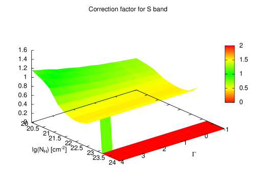
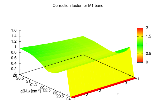
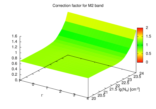
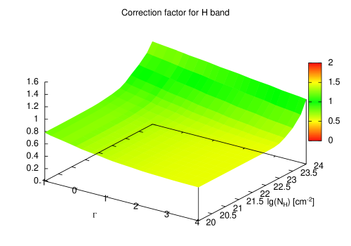
Figure 7.— Surface of correction factors versus spectral parameters for an absorbed power law in the band passes at the aimpoint of the FI ACIS-S3 chip in 2008.

In general the correction is relatively small ($\sim$20–30%). The main variation occurs for large absorption values ($N_{H}>10^{23}$ cm^-2) where the correction factor drops to zero in the soft and medium-soft bands, or strongly increases in the medium-hard band. For practical application, however, a correction factor of zero is not a problem because a zero correction means that there is no flux in that energy band down to computational accuracy ($\int SpdE=0$ in Eq. 14), thus a correction is not useful. Practically, in the code we set incident fluxes to zero if the integral over the spectrum in an energy band is smaller than $10^{-30}$ photons/cm²/s.

Importantly, the shapes of the correction factor surfaces in these plots are similar for different spectral shapes, see Figs. 13, 14, 15 in the Appendix. The difference between two correction surfaces in one band is generally less than $\sim$15%, and never worse than $\sim$40% for the most extreme spectral shapes. Since the spectral shape of a source is a priori unknown, and the point of this work is to not assume any shape, we combine all the points on each grid for all the different spectral shapes. The distribution of correction factors taken from all spectra is shown in Fig.8 for the aimpoint of the BI ACIS-S3 chip in 1999 and 2008. The histograms are strongly peaked, although they have significant tails towards larger correction factors. These tails are especially pronounced in the medium-hard band and are due to spectra with strong absorption values.

Figure 8.— Distribution of correction factors taken from all spectra for aimpoint of ACIS-S3 in 1999 and 2008. Soft band–solid histogram, medium-soft band–dash-dotted histogram, medium-hard band-dashed histogram, hard band–dotted histogram.

Ignoring spectra with large absorption values ($N_{H}>10^{23}$ cm^-2) in the computation of the correction factor has no significant impact on the peak of these distributions but considerably reduces the asymmetry of the distribution for the medium-hard and hard band; the tails almost disappear. This property of highly absorbed spectra may be used in a “color correction” similar to optical photometry. E.g. if there are no counts in the soft and/or medium-soft band, this is already an indication of high absorption, which may be used to change the correction factor distribution in the medium-soft and/or medium-hard and hard band. We address this band ratio correction in a subsequent paper.

Given our ignorance about the intrinsic spectral shape of a source the correction factor distribution can be considered the probability density function $PDF$ of picking the right correction factor for conversion from counts to flux. Thus the probability density function for the correction factors is simply the conjunction of all correction factors $K_{i}$ for a given spectral shape $i$:

$$PDF(K)=\bigwedge_{i}^{N_{sp}}K_{i}.$$ (15)

with $N_{sp}$ the number of different spectra, in this case the sum of parameter combinations from Table 2, and $K_{i}$ the correction factor for spectral parameter combination $i$ according to Eq. 14. Note that $N_{sp}$ has to be sufficiently large to obtain a well behaved distribution. With our choice of spectral shapes and parameters $N_{sp}$ is 1454.

It is important to note here that our selection of spectral shapes serves effectively as a prior on this distribution. This prior is flat in the spectral model/parameter space, i.e. all model/parameter combinations are given equal weight in computing the correction factor distribution. If the correct spectral shape is not covered by this range the method is no longer valid, which is the reason for the large parameter space we use.

Considering the correction factor distribution as a PDF we use the mode of the distribution $\widehat{PDF}$ as the correction factor. As an error estimate we use the range that covers 68% of the distribution as measured from the mode. The mode of the correction factor distribution with the 68% confidence level (CL) errors at the aimpoint of ACIS-S3 for each band for the past 10 years is shown in Fig. 9.

If not noted otherwise all error bars and quoted errors in the following correspond to the 68% confidence level.

4.2. Flux

Using the knowledge of the effects of separate averaging over spectrum and ARF, our ignorance of the true spectral shape of a source, and our estimates for correcting these effects, we can compute a flux estimate $F$ for a source in energy band $i$ at a given location on ACIS as

$$F_{i}=\frac{{C^{\prime}_{s}}_{i}}{\int(ARF\otimes RMF)_{i}dE\cdot T\cdot\widehat{PDF}_{i}}.$$ (16)

with $C^{\prime}_{s}$ as the background subtracted counts corrected for filter overlap in energy band $i$, $ARF$ and $RMF$ the effective area and redistribution matrix in band $i$, $T$ the exposure time, and $\widehat{PDF}_{i}$ the mode of the correction factor distribution in band $i$. $F_{i}$ is in units of photons/s/cm².

4.3. Time variation

Theoretically for Chandra all points on the chips have their own value for the correction factor which in addition is time dependent. Practically, however, the spatial variation across a chip is much smaller than other effects. E.g. the lack of knowledge of the correct spectral shape which is encoded in the variance of the correction factor distribution is of order 15%–20%. Whereas the variation due to changing energy resolution across a chip is about 1%.

Instead temporal changes are important. The change in sensitivity with time significantly affects the effective area and thus the correction factor. Fig. 9 shows the change in the correction factor at the aimpoint of ACIS-S3 for the different energy bands between 1999 and 2007. There is significant change in the correction factor for the soft band up to about 2002 due to accumulation of material. The total change is about 28% between 1999 and 2008, however the medium-hard and hard band are virtually unaffected. The variations for the ACIS-I3 aimpoint are almost identical, except the variation in the soft band is only about 20%.

Figure 9.— Change of correction factor with 68% error bars at the aimpoint of ACIS-S3 between 1999 and 2008. The top panel is the hard band correction factor, second from top medium-hard band correction, third from top medium-soft band correction, and bottom panel the soft band correction. For the soft band the mode of the correction factor distribution is at the lowest value, thus there are no lower error bars (see Fig. 8).

5. Uncertainties

The uncertainties in the X-ray photometry can be separated into statistical and systematic errors. The statistical errors are due only to counting statistics, and so are observation dependent. Due to the fact that our photometry method also deals with small number of counts, Gaussian statistics and error propagation are not appropriate tools. Independent of counting statistics, we consider the distribution of correction factors for a specific chip location and time as a systematic error. This distribution is dependent on the number and kind of spectral shapes and the chip location in time and space.

5.1. Systematic uncertainties

Neither for ARF nor RMF values uncertainties are provided although they are estimated to be below 10%, and around 5% for most of the energy range for the ARF (Drake et al., 2006). We therefore use the correction factor distribution to estimate systematic uncertainties in our program. Individual correction factors are the result of combining spectral shape, ARF, and RMF. Since we use a wide range of spectral shapes and parameters the influence of the spectral shapes/parameters on the uncertainty in flux is certainly much larger than uncertainties in the ARF or RMF.

To obtain the systematic error we choose the mode of the correction factor distribution at a given location of the instrument as the correction factor for that location and integrate from that position in positive and negative direction until 68% of the distribution are covered. In general this will result in asymmetric errors since the distribution is skewed. The flux is inversely proportional to the correction factor, thus the systematic error does not have to be propagated beyond inverting and multiplying by a numerical factor.

5.2. Statistical uncertainties

To obtain the uncertainty on the flux in a band we propagate the errors on the source counts through the corrections applied to the observed counts in a band. In the presence of background we use the method proposed by Kraft et al. (1991) to compute the number of source counts and the uncertainties in that number. Note that the uncertainties are asymmetric and not exactly Poissonian.

Unfortunately there is no obvious or generally accepted way to propagate asymmetric errors. Here we follow the approach of Barlow (2004) for combining asymmetric errors. The approach is based on the idea to parametrize the Log-likelihood curve of the original probability distribution with 3 parameters: Location, scale, and skew for each measurement. Then the Log-likelihood functions for individual measurements are combined, in this case added. Obviously there are numerous ways to parametrize a function through three points. In our program we use the parametrization described as Gaussian with linear variance. This choice is purely empirical and made because this parametrization approximates very well a Poissonian distribution. And although the background subtracted counts and errors are not Poissonian, the difference is quite small. The likelihood function for each part is then given by

$$f(a)=\ln(L(\vec{x};a))=-\frac{1}{2}\frac{a^{2}}{\sigma_{-}\sigma_{+}+(\sigma_{+}-\sigma_{-})a}$$ (17)

where $a$ is the value, and $\sigma_{+-}$ are the asymmetric uncertainties in negative and positive direction.

Combining the likelihood functions for two distributions one can then obtain the combined uncertainties at the locations where $f=f(\hat{a})-\frac{1}{2}$, with $\hat{a}$ being the sum of the counts. Using this method we obtain uncertainties that are slightly larger than assuming Gaussian error propagation for the Gehrels errors (Gehrels, 1986). For large number of counts the error approximates the Gaussian expectation value. Thus we consider our statistical errors to be conservative.

6. Validation

We compare the results of our program with simulated and real data to validate the results and check for variations.

6.1. Simulated data

We simulate 100 spectra each for parameter combinations of two spectral shapes, a black body with a temperature of 0.3 keV and and power law with a photon index of 2. Both spectral shapes have absorption column densities of $10^{20}$ and $10^{22}$ cm^-2. All spectra contain 1000 counts and no background. This is a good approximation for Chandra point sources. The spectra are fitted with Xspec and fluxes are computed using the flux command. These are compared with results from our method.

Results from this comparison are shown in Fig. 10. The figures show Xspec fluxes ($F_{fit}$) over photometric fluxes ($F_{phot}$) computed with our method versus photometric fluxes for the two spectral shapes and four spectral parameter combinations. Different bands are labeled and shown with different symbols. The error bars used correspond to 68% CL. Ideally all y-axis values would be one.

Figure 10.— Comparison between Xspec fluxes ($F_{fit}$) over photometric fluxes ($F_{phot}$) computed with our method versus photometric fluxes for two spectral shapes and four spectral parameter combination. The different bands are noted in the figures, and the right hand figures are cropped for clarity. Ideally all y-axis values would be one. Error bars correspond to 68% CL.

It is clear from the figures that this photometry computes fluxes within better than 30% in most cases, even in the absence of band ratio (color) corrections. That the medium-hard band (M2) has the best correspondence between X-ray photometric fluxes and Xspec fluxes is simply based on the fact that the medium-hard filter has the best properties, very steep edges and a relatively flat top (variation of $\sim$10%) as shown in Fig. 5. Even in the worst cases it is better than 50%. It should be noted that even in the worst cases the systematic error of 68% CL covers the discrepancy between the true and estimated fluxes. The large discrepancies are due to several reasons: (1) a relatively strongly varying spectrum in the energy band, (2) a varying ARF, and (3) differences between the correction factor for that spectrum and the mode of the correction factor distribution. The last factor is quite small, at least for the spectral shapes chosen above. The main contribution to the discrepancy comes from the combination of varying spectrum and ARF and a high number of counts.

With a high number of counts ($>\sim$200) in a band, the changes in the ARF over an energy band become important, particularly for the broad hard band, and the resulting flux differences become significant with respect to the statistical error.

6.2. Real data

The real data we use for our comparison are relatively bright ($>100$ source counts) sources from Chandra observations of M 33. We use two approaches to estimate the flux independently from our method. First we fit the source spectra with spectral models and use the flux command in Xspec to get the photon flux; for best fit models see Grimm et al. (2007).

Secondly we take each photon in an energy band, use the inverse of the ARF at the photon energy, sum this inverse over all photons in the energy band, and divide the result by the exposure time which gives the photon flux. This is the simplest possible photometry method. However, it requires knowledge of individual photon energies, whereas our method works with integrated quantities. This means that the accuracy of this method depends not only on the number of counts, but for weak sources also on where in the energy band the few photons fall. And moreover, it does not take into account effects of the RMF which are important for spectra that produce very different counts in different bands.

Results for sources with well fitted spectra are shown in Fig. 11. The figure shows the flux estimates of our methods as red points, Xspec results as green squares, and summation of inverse effective area as blue triangles. The error bars are 68% CL statistical errors only. In general there is good agreement between all three methods of flux estimation.

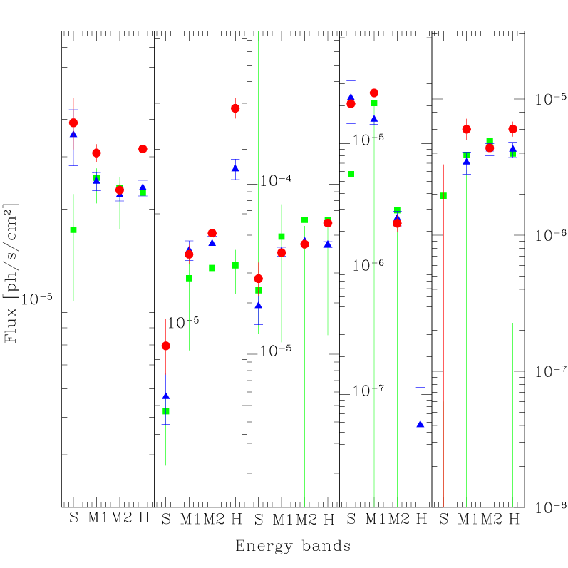
Figure 11.— Flux estimates of our X-ray photometry as (red) circles, Xspec results are (green) squares, and summation of inverse effective area as (blue) triangles versus energy band. Error bars are 68% CL statistical errors.

It is apparent from the figure that there are sometimes significant discrepancies between the flux estimate from our photometry and Xspec fluxes. However the summation of the inverse effective area and our method agree quite well in general. So it is the spectral fitting that results in relatively large deviations from the flux estimates obtained by the other methods. This is probably due to several factors. First, the spectrum is fitted in Xspec using the whole energy range. This can result in an under- or overestimate of fluxes in smaller energy bands, that do not strongly contribute to the overall fit. Furthermore, it can be the case that the chosen spectrum is not a good representation of the data but due to insufficient quality of the data this is not apparent from bad fits. E.g. the spectrum used for the left panel in Fig. 11 has a reduced $\chi^{2}$ of 0.4 which clearly indicates that the bremsstrahlung spectrum chosen for the fit is not the true representation of the data.

7. Conclusion

We have presented a system of X-ray photometry for the Chandra satellite. The system we have developed relies on a knowledge of effective area and the energy-to-channel conversion to construct X-ray filters, but is unbiased by assumptions about the spectral shape of a source. We have shown that the filters are comparable to filters in the optical and infrared, and that our photometric system in X-rays is able to estimate fluxes to within about 20%. Even in the worst cases it is better than 50%. We have incorporated methods to estimate systematic errors and consistently propagate statistical as well as systematic errors.

Due to the construction method employed our filter system is very flexible and can be adapted readily to other CCD X-ray detectors, in particular to XMM-Newton EPIC. The code to compute fluxes is available at a web page . A table with a selection of correction factors for ACIS-S3 is given in Appendix A in the electronic edition and available at the same URL. The table contains only every fourth tile because of the generally slowly varying correction factor with chip location. In the future we will explore potential improvements to X-ray photometry by means of:

• Making color corrections using band ratios. A preliminary investigation suggests that extreme spectra (e.g. highly absorbed or high photon indexes) will gain significantly in the accuracy of flux estimates and even normal spectra will have a reduced error range.

• Optimizing the choice of bands. The properties of our current method show that there is a correlation between the accuracy of flux estimates and the filter shape. The more “boxy” a filter is the better the flux estimate will be. This suggests a limit for the width of a filter at which point deviations from boxiness result in an accuracy of the flux estimate below a certain value.

• Comparing results for Chandra ACIS and XMM-Newton EPIC data. Chandra and XMM have similar instrumental setups (ARF and RMF) and overlapping science capabilities. And given the large numbers of sources observed by these two X-ray missions it is very important to be able to compare results for the two.

8. Acknowledgments

HJG thanks Ralph Kraft for providing the source code for computing confidence limits, and Paul Plucinsky for discussions about the RMF. This work has been supported by NASA grant GO2-3135X and CXC contract NAS8-03060.

Figure 12.— Schematic of the tiling of the full ACIS detector. Direction of the x-axis is indicated by the arrows. The y-axis is counterclockwise to the x-axis. Aimpoints for the I3 and S3 chips are shown as crosses. The readout for chips is on the side of the arrows.

Table 3Correction factors for selected tiles on ACIS-S3.

Tile		Correction factor[keV range]				Tile		Correction factor [keV range]
x	y	0.3–0.5	0.5–1.0	1.0–2.1	2.1–7.5	x	y	0.3–0.5	0.5–1.0	1.0–2.1	2.1–7.5
16	16	$0.39_{-0.00}^{+0.26}$	$0.54_{-0.05}^{+0.18}$	$0.69_{-0.07}^{+0.06}$	$0.54_{-0.07}^{+0.14}$	592	16	$0.40_{-0.00}^{+0.26}$	$0.59_{-0.10}^{+0.13}$	$0.69_{-0.06}^{+0.06}$	$0.54_{-0.07}^{+0.15}$
16	112	$0.45_{-0.01}^{+0.22}$	$0.56_{-0.04}^{+0.19}$	$0.70_{-0.07}^{+0.07}$	$0.54_{-0.07}^{+0.14}$	592	112	$0.45_{-0.01}^{+0.22}$	$0.56_{-0.04}^{+0.19}$	$0.70_{-0.07}^{+0.07}$	$0.54_{-0.07}^{+0.15}$
16	208	$0.47_{-0.01}^{+0.21}$	$0.66_{-0.10}^{+0.11}$	$0.70_{-0.07}^{+0.07}$	$0.54_{-0.06}^{+0.15}$	592	208	$0.47_{-0.01}^{+0.21}$	$0.58_{-0.04}^{+0.17}$	$0.70_{-0.07}^{+0.07}$	$0.54_{-0.06}^{+0.15}$
16	304	$0.47_{-0.01}^{+0.21}$	$0.58_{-0.04}^{+0.17}$	$0.70_{-0.07}^{+0.07}$	$0.54_{-0.06}^{+0.15}$	592	304	$0.47_{-0.00}^{+0.21}$	$0.58_{-0.04}^{+0.17}$	$0.70_{-0.07}^{+0.07}$	$0.54_{-0.06}^{+0.15}$
16	400	$0.47_{-0.01}^{+0.21}$	$0.67_{-0.10}^{+0.11}$	$0.70_{-0.07}^{+0.07}$	$0.54_{-0.06}^{+0.15}$	592	400	$0.48_{-0.01}^{+0.20}$	$0.67_{-0.10}^{+0.11}$	$0.70_{-0.07}^{+0.08}$	$0.54_{-0.06}^{+0.15}$
16	496	$0.47_{-0.01}^{+0.21}$	$0.67_{-0.10}^{+0.11}$	$0.70_{-0.07}^{+0.08}$	$0.55_{-0.07}^{+0.14}$	592	496	$0.48_{-0.01}^{+0.20}$	$0.67_{-0.10}^{+0.11}$	$0.70_{-0.07}^{+0.08}$	$0.55_{-0.07}^{+0.14}$
16	592	$0.48_{-0.01}^{+0.20}$	$0.67_{-0.10}^{+0.10}$	$0.70_{-0.07}^{+0.08}$	$0.53_{-0.05}^{+0.16}$	592	592	$0.48_{-0.01}^{+0.20}$	$0.67_{-0.10}^{+0.10}$	$0.70_{-0.07}^{+0.08}$	$0.53_{-0.05}^{+0.16}$
16	688	$0.48_{-0.01}^{+0.20}$	$0.67_{-0.10}^{+0.10}$	$0.70_{-0.07}^{+0.08}$	$0.55_{-0.07}^{+0.14}$	592	688	$0.48_{-0.01}^{+0.20}$	$0.68_{-0.10}^{+0.11}$	$0.70_{-0.07}^{+0.08}$	$0.55_{-0.07}^{+0.14}$
16	784	$0.48_{-0.01}^{+0.20}$	$0.68_{-0.10}^{+0.11}$	$0.70_{-0.08}^{+0.08}$	$0.55_{-0.08}^{+0.13}$	592	784	$0.48_{-0.01}^{+0.20}$	$0.68_{-0.10}^{+0.11}$	$0.70_{-0.07}^{+0.08}$	$0.55_{-0.08}^{+0.14}$
16	880	$0.47_{-0.01}^{+0.21}$	$0.58_{-0.04}^{+0.17}$	$0.70_{-0.08}^{+0.08}$	$0.55_{-0.09}^{+0.14}$	592	880	$0.47_{-0.01}^{+0.21}$	$0.58_{-0.04}^{+0.17}$	$0.70_{-0.07}^{+0.08}$	$0.55_{-0.08}^{+0.13}$
16	976	$0.44_{-0.01}^{+0.23}$	$0.79_{-0.13}^{+1.29}$	$0.70_{-0.08}^{+0.09}$	$0.55_{-0.09}^{+0.14}$	592	976	$0.44_{-0.01}^{+0.23}$	$0.79_{-0.13}^{+1.30}$	$0.70_{-0.08}^{+0.08}$	$0.55_{-0.09}^{+0.14}$
16	1008	$0.43_{-0.01}^{+0.23}$	$0.56_{-0.04}^{+0.19}$	$0.70_{-0.08}^{+0.09}$	$0.55_{-0.09}^{+0.14}$	592	1008	$0.43_{-0.01}^{+0.24}$	$0.56_{-0.04}^{+0.19}$	$0.70_{-0.08}^{+0.08}$	$0.55_{-0.09}^{+0.14}$
112	16	$0.40_{-0.01}^{+0.26}$	$0.54_{-0.05}^{+0.18}$	$0.69_{-0.07}^{+0.06}$	$0.54_{-0.07}^{+0.14}$	688	16	$0.40_{-0.01}^{+0.26}$	$0.72_{-0.14}^{+1.77}$	$0.69_{-0.06}^{+0.06}$	$0.54_{-0.07}^{+0.15}$
112	112	$0.45_{-0.01}^{+0.22}$	$0.56_{-0.04}^{+0.19}$	$0.70_{-0.07}^{+0.07}$	$0.54_{-0.07}^{+0.14}$	688	112	$0.45_{-0.01}^{+0.22}$	$0.56_{-0.04}^{+0.19}$	$0.70_{-0.07}^{+0.07}$	$0.54_{-0.07}^{+0.15}$
112	208	$0.47_{-0.01}^{+0.21}$	$0.66_{-0.10}^{+0.11}$	$0.70_{-0.07}^{+0.07}$	$0.54_{-0.06}^{+0.14}$	688	208	$0.47_{-0.01}^{+0.21}$	$0.66_{-0.10}^{+0.11}$	$0.70_{-0.07}^{+0.07}$	$0.54_{-0.07}^{+0.15}$
112	304	$0.47_{-0.00}^{+0.21}$	$0.58_{-0.04}^{+0.17}$	$0.70_{-0.07}^{+0.07}$	$0.54_{-0.06}^{+0.15}$	688	304	$0.48_{-0.01}^{+0.20}$	$0.58_{-0.04}^{+0.17}$	$0.70_{-0.07}^{+0.07}$	$0.54_{-0.07}^{+0.15}$
112	400	$0.48_{-0.01}^{+0.20}$	$0.58_{-0.04}^{+0.17}$	$0.70_{-0.07}^{+0.07}$	$0.54_{-0.06}^{+0.15}$	688	400	$0.48_{-0.01}^{+0.20}$	$0.58_{-0.04}^{+0.17}$	$0.70_{-0.07}^{+0.07}$	$0.54_{-0.06}^{+0.15}$
112	496	$0.48_{-0.01}^{+0.20}$	$0.58_{-0.04}^{+0.17}$	$0.70_{-0.07}^{+0.07}$	$0.54_{-0.06}^{+0.15}$	688	496	$0.48_{-0.01}^{+0.20}$	$0.58_{-0.04}^{+0.17}$	$0.70_{-0.07}^{+0.07}$	$0.54_{-0.06}^{+0.15}$
112	592	$0.48_{-0.01}^{+0.20}$	$0.67_{-0.10}^{+0.11}$	$0.70_{-0.07}^{+0.08}$	$0.55_{-0.07}^{+0.14}$	688	592	$0.48_{-0.01}^{+0.20}$	$0.58_{-0.04}^{+0.17}$	$0.70_{-0.07}^{+0.07}$	$0.53_{-0.05}^{+0.16}$
112	688	$0.48_{-0.01}^{+0.20}$	$0.67_{-0.10}^{+0.11}$	$0.70_{-0.07}^{+0.08}$	$0.55_{-0.07}^{+0.14}$	688	688	$0.48_{-0.01}^{+0.20}$	$0.67_{-0.10}^{+0.11}$	$0.70_{-0.07}^{+0.08}$	$0.53_{-0.06}^{+0.16}$
112	784	$0.47_{-0.01}^{+0.21}$	$0.58_{-0.04}^{+0.17}$	$0.70_{-0.07}^{+0.08}$	$0.53_{-0.05}^{+0.16}$	688	784	$0.47_{-0.00}^{+0.21}$	$0.67_{-0.10}^{+0.11}$	$0.70_{-0.07}^{+0.08}$	$0.55_{-0.08}^{+0.14}$
112	880	$0.47_{-0.02}^{+0.20}$	$0.66_{-0.10}^{+0.11}$	$0.70_{-0.08}^{+0.08}$	$0.55_{-0.08}^{+0.14}$	688	880	$0.46_{-0.00}^{+0.22}$	$0.58_{-0.04}^{+0.17}$	$0.70_{-0.07}^{+0.08}$	$0.55_{-0.08}^{+0.14}$
112	976	$0.44_{-0.01}^{+0.23}$	$0.56_{-0.04}^{+0.19}$	$0.70_{-0.08}^{+0.07}$	$0.55_{-0.09}^{+0.14}$	688	976	$0.44_{-0.01}^{+0.23}$	$0.79_{-0.13}^{+1.31}$	$0.70_{-0.07}^{+0.08}$	$0.55_{-0.09}^{+0.14}$
112	1008	$0.43_{-0.01}^{+0.23}$	$0.55_{-0.04}^{+0.20}$	$0.70_{-0.08}^{+0.08}$	$0.55_{-0.09}^{+0.14}$	688	1008	$0.43_{-0.01}^{+0.24}$	$0.63_{-0.10}^{+0.13}$	$0.70_{-0.08}^{+0.08}$	$0.55_{-0.09}^{+0.14}$
208	16	$0.40_{-0.01}^{+0.26}$	$0.54_{-0.05}^{+0.18}$	$0.69_{-0.07}^{+0.06}$	$0.54_{-0.07}^{+0.14}$	784	16	$0.41_{-0.00}^{+0.26}$	$0.59_{-0.10}^{+0.13}$	$0.69_{-0.07}^{+0.06}$	$0.54_{-0.07}^{+0.15}$
208	112	$0.44_{-0.01}^{+0.23}$	$0.63_{-0.10}^{+0.12}$	$0.70_{-0.07}^{+0.07}$	$0.54_{-0.06}^{+0.14}$	784	112	$0.46_{-0.01}^{+0.22}$	$0.79_{-0.13}^{+1.28}$	$0.70_{-0.07}^{+0.07}$	$0.54_{-0.07}^{+0.15}$
208	208	$0.46_{-0.01}^{+0.21}$	$0.72_{-0.11}^{+0.18}$	$0.70_{-0.07}^{+0.07}$	$0.54_{-0.06}^{+0.14}$	784	208	$0.48_{-0.01}^{+0.20}$	$0.58_{-0.04}^{+0.17}$	$0.70_{-0.07}^{+0.07}$	$0.53_{-0.06}^{+0.16}$
208	304	$0.47_{-0.01}^{+0.20}$	$0.66_{-0.10}^{+0.11}$	$0.70_{-0.07}^{+0.07}$	$0.54_{-0.06}^{+0.14}$	784	304	$0.48_{-0.01}^{+0.21}$	$0.67_{-0.10}^{+0.10}$	$0.70_{-0.07}^{+0.07}$	$0.53_{-0.06}^{+0.16}$
208	400	$0.47_{-0.01}^{+0.20}$	$0.58_{-0.04}^{+0.17}$	$0.70_{-0.07}^{+0.07}$	$0.54_{-0.06}^{+0.14}$	784	400	$0.48_{-0.01}^{+0.21}$	$0.67_{-0.10}^{+0.10}$	$0.70_{-0.07}^{+0.07}$	$0.53_{-0.06}^{+0.16}$
208	496	$0.47_{-0.01}^{+0.21}$	$0.58_{-0.04}^{+0.17}$	$0.70_{-0.07}^{+0.07}$	$0.56_{-0.09}^{+0.13}$	784	496	$0.48_{-0.01}^{+0.21}$	$0.62_{-0.07}^{+0.13}$	$0.70_{-0.07}^{+0.07}$	$0.55_{-0.08}^{+0.14}$
208	592	$0.47_{-0.01}^{+0.21}$	$0.58_{-0.04}^{+0.17}$	$0.70_{-0.07}^{+0.07}$	$0.55_{-0.07}^{+0.14}$	784	592	$0.48_{-0.00}^{+0.21}$	$0.68_{-0.10}^{+0.11}$	$0.70_{-0.07}^{+0.07}$	$0.55_{-0.08}^{+0.14}$
208	688	$0.47_{-0.01}^{+0.21}$	$0.58_{-0.04}^{+0.17}$	$0.70_{-0.07}^{+0.07}$	$0.55_{-0.07}^{+0.14}$	784	688	$0.49_{-0.01}^{+0.20}$	$0.68_{-0.10}^{+0.11}$	$0.70_{-0.07}^{+0.08}$	$0.55_{-0.08}^{+0.14}$
208	784	$0.47_{-0.01}^{+0.21}$	$0.58_{-0.04}^{+0.17}$	$0.70_{-0.07}^{+0.08}$	$0.55_{-0.07}^{+0.14}$	784	784	$0.48_{-0.01}^{+0.21}$	$0.59_{-0.04}^{+0.16}$	$0.70_{-0.07}^{+0.08}$	$0.55_{-0.09}^{+0.14}$
208	880	$0.46_{-0.01}^{+0.21}$	$0.81_{-0.13}^{+1.14}$	$0.70_{-0.07}^{+0.07}$	$0.53_{-0.06}^{+0.16}$	784	880	$0.48_{-0.01}^{+0.20}$	$0.58_{-0.04}^{+0.17}$	$0.70_{-0.08}^{+0.08}$	$0.55_{-0.09}^{+0.14}$
208	976	$0.44_{-0.01}^{+0.23}$	$0.56_{-0.04}^{+0.19}$	$0.70_{-0.08}^{+0.07}$	$0.55_{-0.08}^{+0.14}$	784	976	$0.45_{-0.01}^{+0.23}$	$0.79_{-0.13}^{+1.31}$	$0.70_{-0.08}^{+0.07}$	$0.54_{-0.07}^{+0.14}$
208	1008	$0.43_{-0.01}^{+0.23}$	$0.55_{-0.04}^{+0.20}$	$0.70_{-0.08}^{+0.07}$	$0.55_{-0.08}^{+0.14}$	784	1008	$0.44_{-0.01}^{+0.23}$	$0.56_{-0.04}^{+0.19}$	$0.70_{-0.08}^{+0.07}$	$0.52_{-0.06}^{+0.16}$
304	16	$0.41_{-0.00}^{+0.26}$	$0.53_{-0.04}^{+0.20}$	$0.69_{-0.06}^{+0.06}$	$0.54_{-0.06}^{+0.15}$	880	16	$0.41_{-0.01}^{+0.25}$	$0.72_{-0.14}^{+1.77}$	$0.69_{-0.07}^{+0.06}$	$0.55_{-0.09}^{+0.14}$
304	112	$0.46_{-0.01}^{+0.22}$	$0.79_{-0.13}^{+1.27}$	$0.70_{-0.07}^{+0.07}$	$0.54_{-0.06}^{+0.15}$	880	112	$0.46_{-0.01}^{+0.21}$	$0.79_{-0.13}^{+1.28}$	$0.70_{-0.07}^{+0.07}$	$0.55_{-0.09}^{+0.14}$
304	208	$0.48_{-0.01}^{+0.21}$	$0.58_{-0.04}^{+0.17}$	$0.70_{-0.07}^{+0.07}$	$0.54_{-0.06}^{+0.15}$	880	208	$0.48_{-0.01}^{+0.20}$	$0.58_{-0.04}^{+0.17}$	$0.70_{-0.07}^{+0.07}$	$0.55_{-0.09}^{+0.14}$
304	304	$0.48_{-0.00}^{+0.21}$	$0.67_{-0.10}^{+0.11}$	$0.70_{-0.07}^{+0.07}$	$0.54_{-0.06}^{+0.15}$	880	304	$0.48_{-0.01}^{+0.21}$	$0.67_{-0.10}^{+0.11}$	$0.70_{-0.07}^{+0.07}$	$0.55_{-0.09}^{+0.14}$
304	400	$0.48_{-0.00}^{+0.22}$	$0.67_{-0.10}^{+0.11}$	$0.70_{-0.07}^{+0.07}$	$0.54_{-0.06}^{+0.15}$	880	400	$0.48_{-0.01}^{+0.21}$	$0.67_{-0.10}^{+0.10}$	$0.70_{-0.07}^{+0.07}$	$0.55_{-0.09}^{+0.14}$
304	496	$0.48_{-0.00}^{+0.22}$	$0.67_{-0.10}^{+0.10}$	$0.70_{-0.07}^{+0.07}$	$0.56_{-0.08}^{+0.13}$	880	496	$0.48_{-0.00}^{+0.21}$	$0.67_{-0.10}^{+0.10}$	$0.70_{-0.07}^{+0.07}$	$0.55_{-0.09}^{+0.14}$
304	592	$0.48_{-0.00}^{+0.22}$	$0.68_{-0.10}^{+0.11}$	$0.70_{-0.07}^{+0.07}$	$0.56_{-0.08}^{+0.13}$	880	592	$0.48_{-0.01}^{+0.21}$	$0.67_{-0.10}^{+0.10}$	$0.70_{-0.07}^{+0.07}$	$0.55_{-0.09}^{+0.14}$
304	688	$0.49_{-0.01}^{+0.21}$	$0.68_{-0.10}^{+0.11}$	$0.70_{-0.07}^{+0.08}$	$0.56_{-0.08}^{+0.13}$	880	688	$0.48_{-0.01}^{+0.21}$	$0.67_{-0.10}^{+0.10}$	$0.70_{-0.07}^{+0.08}$	$0.55_{-0.09}^{+0.14}$
304	784	$0.48_{-0.00}^{+0.22}$	$0.68_{-0.10}^{+0.11}$	$0.70_{-0.07}^{+0.08}$	$0.56_{-0.09}^{+0.13}$	880	784	$0.48_{-0.01}^{+0.21}$	$0.67_{-0.10}^{+0.10}$	$0.70_{-0.08}^{+0.08}$	$0.54_{-0.07}^{+0.14}$
304	880	$0.48_{-0.01}^{+0.21}$	$0.58_{-0.04}^{+0.17}$	$0.70_{-0.07}^{+0.07}$	$0.55_{-0.07}^{+0.14}$	880	880	$0.47_{-0.01}^{+0.21}$	$0.58_{-0.04}^{+0.17}$	$0.70_{-0.08}^{+0.08}$	$0.55_{-0.09}^{+0.15}$
304	976	$0.46_{-0.01}^{+0.22}$	$0.79_{-0.13}^{+1.32}$	$0.70_{-0.07}^{+0.07}$	$0.53_{-0.06}^{+0.16}$	880	976	$0.45_{-0.01}^{+0.23}$	$0.79_{-0.13}^{+1.31}$	$0.70_{-0.08}^{+0.07}$	$0.55_{-0.08}^{+0.16}$
304	1008	$0.45_{-0.01}^{+0.23}$	$0.63_{-0.10}^{+0.13}$	$0.70_{-0.07}^{+0.07}$	$0.53_{-0.06}^{+0.16}$	880	1008	$0.44_{-0.01}^{+0.23}$	$0.63_{-0.10}^{+0.13}$	$0.70_{-0.08}^{+0.07}$	$0.55_{-0.08}^{+0.16}$
400	16	$0.42_{-0.01}^{+0.25}$	$0.59_{-0.10}^{+0.13}$	$0.69_{-0.06}^{+0.06}$	$0.54_{-0.07}^{+0.15}$	976	16	$0.41_{-0.01}^{+0.25}$	$0.59_{-0.10}^{+0.13}$	$0.69_{-0.07}^{+0.06}$	$0.55_{-0.09}^{+0.14}$
400	112	$0.47_{-0.02}^{+0.21}$	$0.79_{-0.13}^{+1.27}$	$0.70_{-0.07}^{+0.07}$	$0.54_{-0.06}^{+0.15}$	976	112	$0.46_{-0.01}^{+0.22}$	$0.79_{-0.13}^{+1.27}$	$0.70_{-0.06}^{+0.07}$	$0.55_{-0.09}^{+0.14}$
400	208	$0.48_{-0.00}^{+0.21}$	$0.58_{-0.04}^{+0.17}$	$0.70_{-0.07}^{+0.07}$	$0.54_{-0.06}^{+0.15}$	976	208	$0.48_{-0.01}^{+0.21}$	$0.58_{-0.04}^{+0.17}$	$0.70_{-0.07}^{+0.07}$	$0.55_{-0.09}^{+0.14}$
400	304	$0.49_{-0.01}^{+0.21}$	$0.67_{-0.10}^{+0.11}$	$0.70_{-0.07}^{+0.07}$	$0.54_{-0.06}^{+0.15}$	976	304	$0.49_{-0.01}^{+0.21}$	$0.67_{-0.10}^{+0.10}$	$0.70_{-0.08}^{+0.07}$	$0.54_{-0.08}^{+0.14}$
400	400	$0.49_{-0.01}^{+0.21}$	$0.67_{-0.10}^{+0.10}$	$0.70_{-0.07}^{+0.07}$	$0.56_{-0.08}^{+0.13}$	976	400	$0.49_{-0.01}^{+0.21}$	$0.67_{-0.10}^{+0.10}$	$0.70_{-0.07}^{+0.08}$	$0.55_{-0.09}^{+0.15}$
400	496	$0.49_{-0.01}^{+0.21}$	$0.67_{-0.10}^{+0.10}$	$0.70_{-0.07}^{+0.07}$	$0.56_{-0.08}^{+0.13}$	976	496	$0.49_{-0.01}^{+0.21}$	$0.68_{-0.10}^{+0.11}$	$0.70_{-0.07}^{+0.08}$	$0.55_{-0.09}^{+0.15}$
400	592	$0.49_{-0.01}^{+0.21}$	$0.68_{-0.10}^{+0.11}$	$0.70_{-0.07}^{+0.07}$	$0.56_{-0.09}^{+0.13}$	976	592	$0.49_{-0.01}^{+0.21}$	$0.68_{-0.10}^{+0.11}$	$0.70_{-0.08}^{+0.08}$	$0.55_{-0.08}^{+0.16}$
400	688	$0.49_{-0.01}^{+0.21}$	$0.68_{-0.10}^{+0.11}$	$0.70_{-0.07}^{+0.08}$	$0.55_{-0.07}^{+0.14}$	976	688	$0.49_{-0.01}^{+0.21}$	$0.68_{-0.10}^{+0.11}$	$0.70_{-0.07}^{+0.09}$	$0.55_{-0.08}^{+0.17}$
400	784	$0.49_{-0.01}^{+0.21}$	$0.68_{-0.10}^{+0.11}$	$0.70_{-0.07}^{+0.08}$	$0.56_{-0.09}^{+0.14}$	976	784	$0.48_{-0.00}^{+0.22}$	$0.68_{-0.10}^{+0.11}$	$0.70_{-0.05}^{+0.09}$	$0.50_{-0.04}^{+0.18}$
400	880	$0.48_{-0.01}^{+0.21}$	$0.58_{-0.04}^{+0.17}$	$0.70_{-0.07}^{+0.08}$	$0.53_{-0.05}^{+0.16}$	976	880	$0.48_{-0.01}^{+0.21}$	$0.67_{-0.10}^{+0.11}$	$0.70_{-0.08}^{+0.09}$	$0.50_{-0.04}^{+0.18}$
400	976	$0.46_{-0.01}^{+0.22}$	$0.57_{-0.04}^{+0.19}$	$0.70_{-0.07}^{+0.08}$	$0.55_{-0.08}^{+0.14}$	976	976	$0.46_{-0.01}^{+0.22}$	$0.57_{-0.04}^{+0.18}$	$0.70_{-0.08}^{+0.08}$	$0.50_{-0.04}^{+0.18}$
400	1008	$0.45_{-0.01}^{+0.23}$	$0.56_{-0.04}^{+0.19}$	$0.70_{-0.08}^{+0.07}$	$0.55_{-0.08}^{+0.14}$	976	1008	$0.44_{-0.00}^{+0.23}$	$0.56_{-0.04}^{+0.19}$	$0.70_{-0.08}^{+0.08}$	$0.50_{-0.04}^{+0.18}$
496	16	$0.42_{-0.01}^{+0.25}$	$0.53_{-0.04}^{+0.20}$	$0.69_{-0.06}^{+0.06}$	$0.54_{-0.07}^{+0.15}$	1008	16	$0.40_{-0.00}^{+0.26}$	$0.59_{-0.10}^{+0.13}$	$0.69_{-0.07}^{+0.06}$	$0.54_{-0.08}^{+0.15}$
496	112	$0.47_{-0.01}^{+0.21}$	$0.71_{-0.12}^{+0.13}$	$0.70_{-0.07}^{+0.07}$	$0.54_{-0.06}^{+0.15}$	1008	112	$0.46_{-0.01}^{+0.22}$	$0.71_{-0.11}^{+0.13}$	$0.70_{-0.08}^{+0.07}$	$0.52_{-0.06}^{+0.17}$
496	208	$0.48_{-0.00}^{+0.22}$	$0.67_{-0.10}^{+0.11}$	$0.70_{-0.07}^{+0.07}$	$0.54_{-0.06}^{+0.15}$	1008	208	$0.48_{-0.00}^{+0.21}$	$0.67_{-0.10}^{+0.11}$	$0.70_{-0.07}^{+0.07}$	$0.54_{-0.08}^{+0.14}$
496	304	$0.49_{-0.01}^{+0.21}$	$0.68_{-0.10}^{+0.11}$	$0.70_{-0.07}^{+0.07}$	$0.54_{-0.06}^{+0.15}$	1008	304	$0.49_{-0.01}^{+0.21}$	$0.68_{-0.10}^{+0.11}$	$0.70_{-0.07}^{+0.08}$	$0.54_{-0.08}^{+0.14}$
496	400	$0.49_{-0.00}^{+0.21}$	$0.59_{-0.04}^{+0.16}$	$0.70_{-0.07}^{+0.08}$	$0.55_{-0.07}^{+0.14}$	1008	400	$0.49_{-0.01}^{+0.21}$	$0.68_{-0.10}^{+0.11}$	$0.70_{-0.08}^{+0.08}$	$0.54_{-0.08}^{+0.14}$
496	496	$0.49_{-0.01}^{+0.21}$	$0.59_{-0.04}^{+0.17}$	$0.70_{-0.07}^{+0.08}$	$0.55_{-0.07}^{+0.14}$	1008	496	$0.49_{-0.01}^{+0.21}$	$0.59_{-0.04}^{+0.17}$	$0.70_{-0.08}^{+0.08}$	$0.55_{-0.08}^{+0.16}$
496	592	$0.49_{-0.01}^{+0.21}$	$0.59_{-0.04}^{+0.16}$	$0.70_{-0.07}^{+0.08}$	$0.55_{-0.07}^{+0.14}$	1008	592	$0.49_{-0.01}^{+0.21}$	$0.59_{-0.04}^{+0.17}$	$0.70_{-0.08}^{+0.09}$	$0.54_{-0.08}^{+0.14}$
496	688	$0.49_{-0.01}^{+0.21}$	$0.59_{-0.04}^{+0.17}$	$0.70_{-0.07}^{+0.08}$	$0.53_{-0.05}^{+0.16}$	1008	688	$0.49_{-0.01}^{+0.21}$	$0.59_{-0.04}^{+0.17}$	$0.70_{-0.03}^{+0.10}$	$0.50_{-0.04}^{+0.18}$
496	784	$0.49_{-0.01}^{+0.21}$	$0.68_{-0.10}^{+0.11}$	$0.70_{-0.07}^{+0.08}$	$0.55_{-0.07}^{+0.14}$	1008	784	$0.49_{-0.01}^{+0.21}$	$0.59_{-0.04}^{+0.17}$	$0.70_{-0.02}^{+0.11}$	$0.50_{-0.04}^{+0.18}$
496	880	$0.48_{-0.01}^{+0.21}$	$0.58_{-0.04}^{+0.17}$	$0.70_{-0.07}^{+0.08}$	$0.55_{-0.08}^{+0.14}$	1008	880	$0.48_{-0.01}^{+0.21}$	$0.68_{-0.10}^{+0.11}$	$0.70_{-0.04}^{+0.10}$	$0.50_{-0.04}^{+0.19}$
496	976	$0.46_{-0.01}^{+0.22}$	$0.57_{-0.04}^{+0.19}$	$0.70_{-0.08}^{+0.08}$	$0.55_{-0.09}^{+0.14}$	1008	976	$0.46_{-0.01}^{+0.22}$	$0.81_{-0.13}^{+1.26}$	$0.70_{-0.08}^{+0.09}$	$0.50_{-0.04}^{+0.18}$
496	1008	$0.45_{-0.01}^{+0.23}$	$0.56_{-0.04}^{+0.20}$	$0.70_{-0.08}^{+0.08}$	$0.55_{-0.09}^{+0.14}$	1008	1008	$0.44_{-0.01}^{+0.23}$	$0.79_{-0.13}^{+1.37}$	$0.70_{-0.08}^{+0.09}$	$0.54_{-0.09}^{+0.15}$

^a – X and Y are the tile center in chip coordinates.
^b – Values are the mode of the correction factor distribution (Eq.15) with the 68% CL error (see Sec. 4.1 & 5.1). The values should be used as input in Eq. 16.
^c – Aimpoint on ACIS-S3

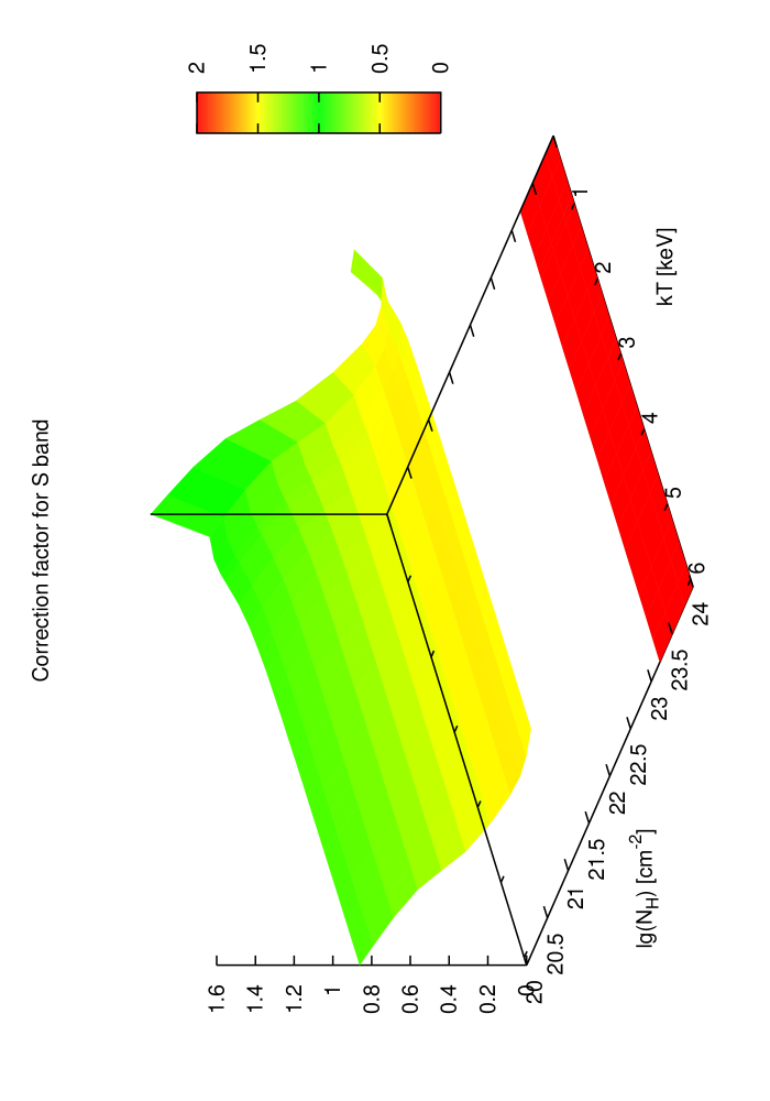
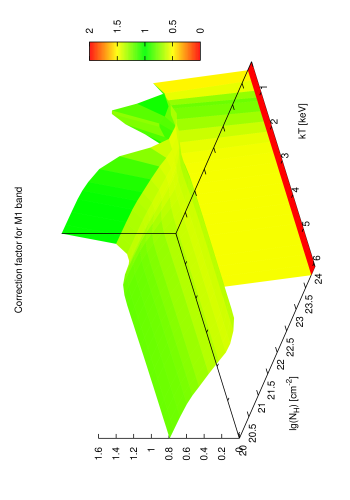
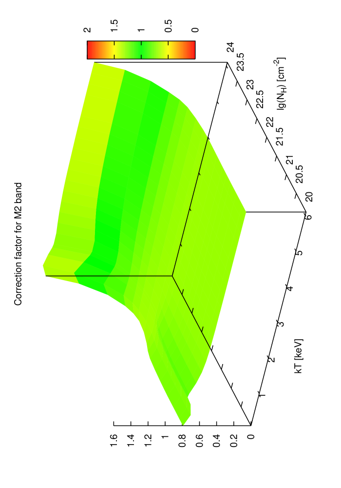
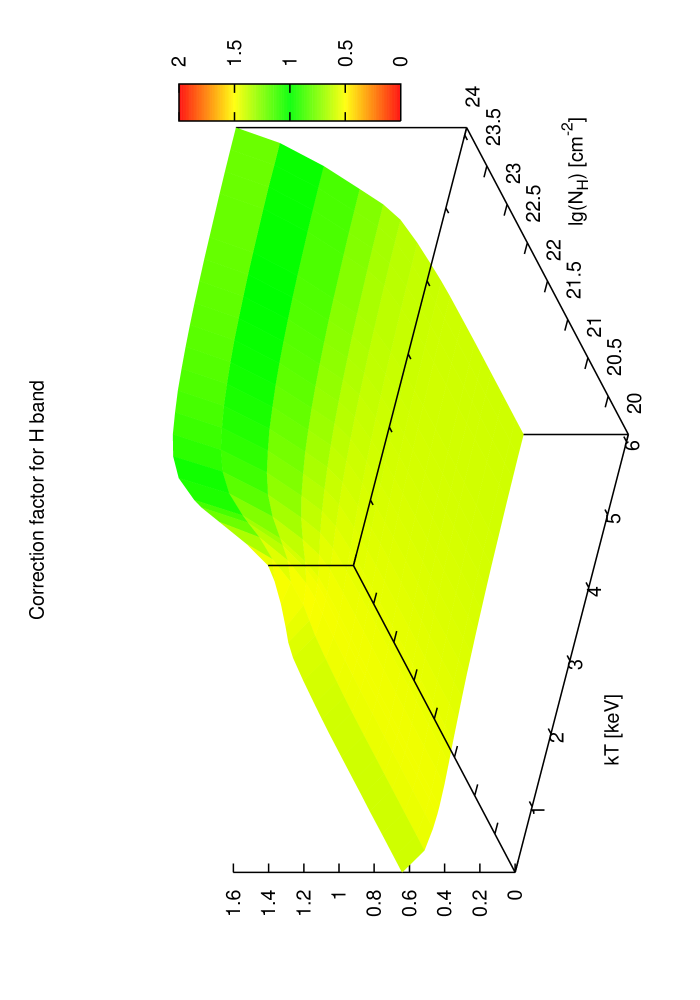
Figure 13.— Surface of correction factors versus spectral parameters for an absorbed thermal plasma spectrum (APEC model) in the band passes at the aimpoint of the FI ACIS-S3 chip in 2008.

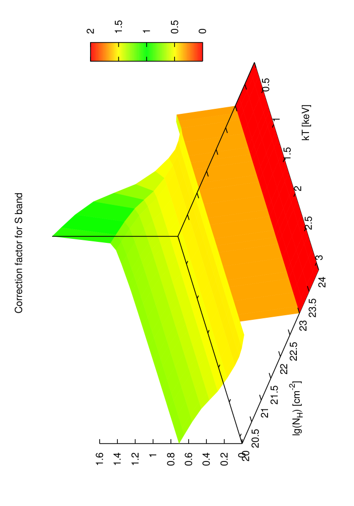
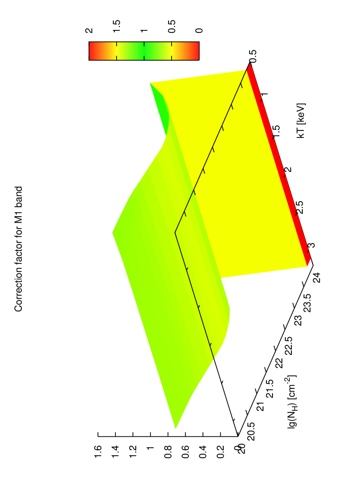
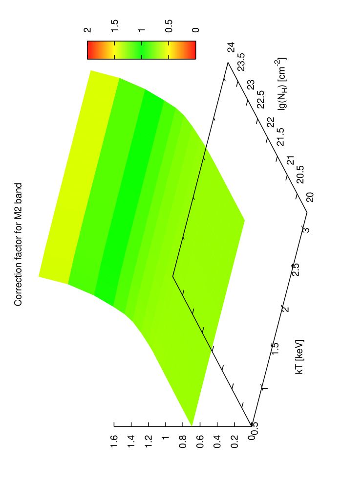
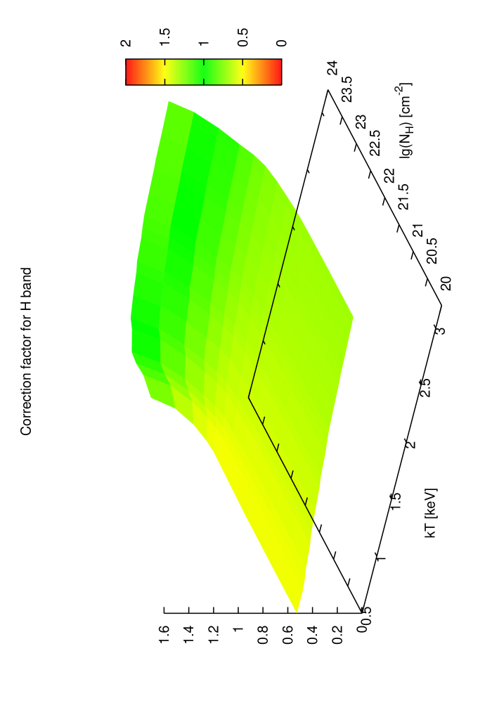
Figure 14.— Surface of correction factors versus spectral parameters for an absorbed black body spectrum in the band passes at the aimpoint of the FI ACIS-S3 chip in 2008.

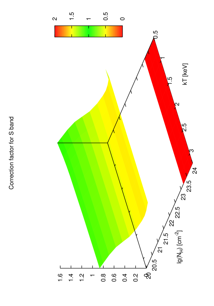
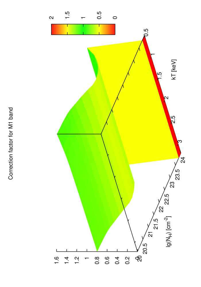
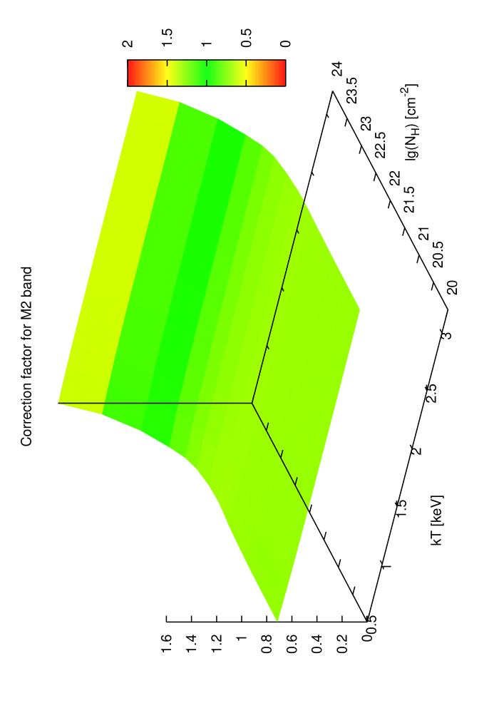
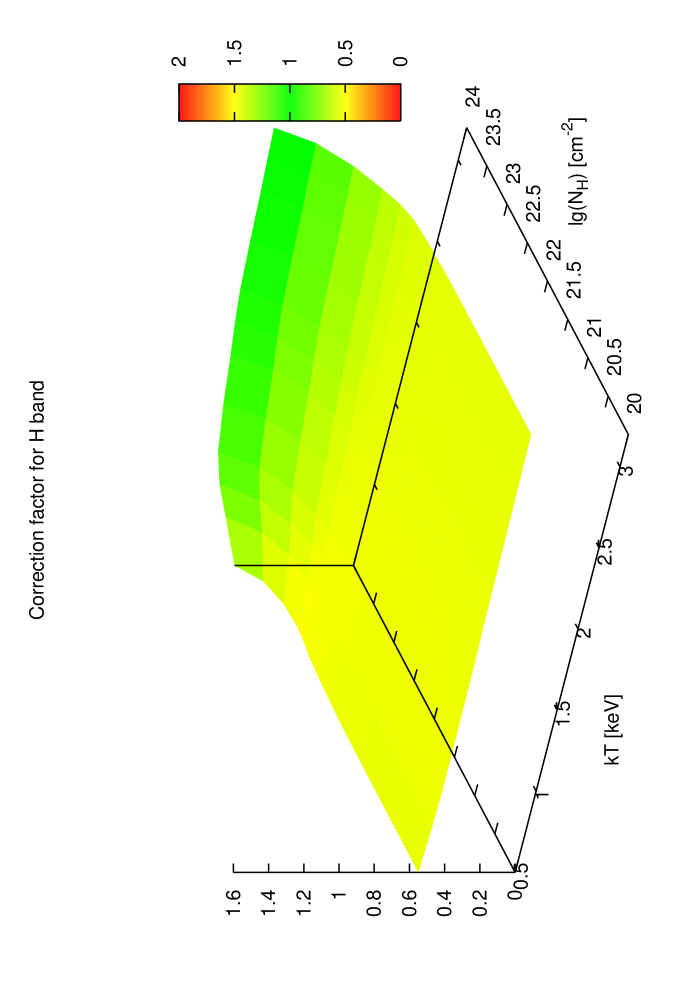
Figure 15.— Surface of correction factors versus spectral parameters for an absorbed bremsstrahlung spectrum in the band passes at the aimpoint of the FI ACIS-S3 chip in 2008.

References

- Barlow (2004) Barlow, R. 2004, ArXiv Physics e-prints
- Bautz et al. (1999) Bautz, M. W., Prigozhin, G. Y., Pivovaroff, M. J., Jones, S. E., Kissel, S. E., & Ricker, G. R. 1999, Nuclear Instruments and Methods in Physics Research A, 436, 40
- Bessell (2005) Bessell, M. S. 2005, ARA&A, 43, 293
- Burke et al. (1993) Burke, B. E., Mountain, R. W., Daniels, P. J., Cooper, M. J., & Dolat, V. S. 1993, in Presented at the Society of Photo-Optical Instrumentation Engineers (SPIE) Conference, Vol. 2006, Proc. SPIE Vol. 2006, p. 272-285, EUV, X-Ray, and Gamma-Ray Instrumentation for Astronomy IV, Oswald H. Siegmund; Ed., ed. O. H. Siegmund, 272–285
- CXC (2008) CXC. 2008, The Chandra Proposers’ Observatory Guide, 10th edn., Chandra X-ray Center, http://cxc.harvard.edu/proposer/POG/html/index.html
- Drake et al. (2006) Drake, J. J., Ratzlaff, P., Kashyap, V., Edgar, R., Izem, R., Jerius, D., Siemiginowska, A., & Vikhlinin, A. 2006, in Presented at the Society of Photo-Optical Instrumentation Engineers (SPIE) Conference, Vol. 6270, Observatory Operations: Strategies, Processes, and Systems. Edited by Silva, David R.; Doxsey, Rodger E.. Proceedings of the SPIE, Volume 6270, pp. 62701I (2006).
- Fabbiano et al. (2007) Fabbiano, G., Evans, I., Evans, J., Glotfelty, K., Hain, R., McCollough, M., Primini, F., Rots, A., Calderwood, T., Doe, S., Grier, J., Harbo, P., Karovska, M., McDowell, J., Plummer, D., Paton, L., Tibbetts, M., Stone, D. V., & Zografou, P. 2007, in Astronomical Society of the Pacific Conference Series, Vol. 376, Astronomical Society of the Pacific Conference Series, ed. R. A. Shaw, F. Hill, & D. J. Bell, 172–+
- Fan et al. (1999) Fan, X., Strauss, M. A., Schneider, D. P., Gunn, J. E., Lupton, R. H., Yanny, B., Anderson, S. F., Anderson, Jr., J. E., Annis, J., Bahcall, N. A., Bakken, J. A., Bastian, S., Berman, E., Boroski, W. N., Briegel, C., Briggs, J. W., Brinkmann, J., Carr, M. A., Colestock, P. L., Connolly, A. J., Crocker, J. H., Csabai, I., Czarapata, P. C., Davis, J. E., Doi, M., Elms, B. R., Evans, M. L., Federwitz, G. R., Frieman, J. A., Fukugita, M., Gurbani, V. K., Harris, F. H., Heckman, T. M., Hennessy, G. S., Hindsley, R. B., Holmgren, D. J., Hull, C., Ichikawa, S.-I., Ichikawa, T., Ivezić , Ž., Kent, S., Knapp, G. R., Kron, R. G., Lamb, D. Q., Leger, R. F., Limmongkol, S., Lindenmeyer, C., Long, D. C., Loveday, J., MacKinnon, B., Mannery, E. J., Mantsch, P. M., Margon, B., McKay, T. A., Munn, J. A., Nash, T., Newberg, H. J., Nichol, R. C., Nicinski, T., Okamura, S., Ostriker, J. P., Owen, R., Pauls, A. G., Peoples, J., Petravick, D., Pier, J. R., Pordes, R., Prosapio, A., Rechenmacher, R., Richards, G. T., Richmond, M. W., Rivetta, C. H., Rockosi, C. M., Sandford, D., Sergey, G., Sekiguchi, M., Shimasaku, K., Siegmund, W. A., Smith, J. A., Stoughton, C., Szalay, A. S., Szokoly, G. P., Tucker, D. L., Vogeley, M. S., Waddell, P., Wang, S.-I., Weinberg, D. H., Yasuda, N., & York, D. G. 1999, AJ, 118, 1
- Gehrels (1986) Gehrels, N. 1986, ApJ, 303, 336
- Gierliński & Newton (2006) Gierliński, M. & Newton, J. 2006, MNRAS, 370, 837
- Grimm et al. (2007) Grimm, H.-J., McDowell, J., Zezas, A., Kim, D.-W., & Fabbiano, G. 2007, ApJS, 173, 70
- Hasinger & van der Klis (1989) Hasinger, G. & van der Klis, M. 1989, A&A, 225, 79
- Johnson & Morgan (1953) Johnson, H. L. & Morgan, W. W. 1953, ApJ, 117, 313
- Kraft et al. (1991) Kraft, R. P., Burrows, D. N., & Nousek, J. A. 1991, ApJ, 374, 344
- Marshall et al. (2004) Marshall, H. L., Tennant, A., Grant, C. E., Hitchcock, A. P., O’Dell, S. L., & Plucinsky, P. P. 2004, in Presented at the Society of Photo-Optical Instrumentation Engineers (SPIE) Conference, Vol. 5165, X-Ray and Gamma-Ray Instrumentation for Astronomy XIII. Edited by Flanagan, Kathryn A.; Siegmund, Oswald H. W. Proceedings of the SPIE, Volume 5165, pp. 497-508 (2004)., ed. K. A. Flanagan & O. H. W. Siegmund, 497–508
- Plucinsky et al. (2003) Plucinsky, P. P., Schulz, N. S., Marshall, H. L., Grant, C. E., Chartas, G., Sanwal, D., Teter, M., Vikhlinin, A. A., Edgar, R. J., Wise, M. W., Allen, G. E., Virani, S. N., DePasquale, J. M., & Raley, M. T. 2003, in Presented at the Society of Photo-Optical Instrumentation Engineers (SPIE) Conference, Vol. 4851, X-Ray and Gamma-Ray Telescopes and Instruments for Astronomy. Edited by Joachim E. Truemper, Harvey D. Tananbaum. Proceedings of the SPIE, Volume 4851, pp. 89-100 (2003)., ed. J. E. Truemper & H. D. Tananbaum, 89–100
- Prestwich et al. (2003) Prestwich, A. H., Irwin, J. A., Kilgard, R. E., Krauss, M. I., Zezas, A., Primini, F., Kaaret, P., & Boroson, B. 2003, ApJ, 595, 719
- Prigozhin et al. (1998) Prigozhin, G. Y., Rasmussen, A., Bautz, M. W., & Ricker, G. R. 1998, in Presented at the Society of Photo-Optical Instrumentation Engineers (SPIE) Conference, Vol. 3444, Proc. SPIE Vol. 3444, p. 267-275, X-Ray Optics, Instruments, and Missions, Richard B. Hoover; Arthur B. Walker; Eds., ed. R. B. Hoover & A. B. Walker, 267–275
- Puschell et al. (1981) Puschell, J. J., Owen, F. N., & Laing, R. A. 1981, in Bulletin of the American Astronomical Society, Vol. 13, Bulletin of the American Astronomical Society, 507–+
- Schwartz et al. (2000) Schwartz, D. A., David, L. P., Donnelly, R. H., Edgar, R. J., Gaetz, T. J., Graessle, D. E., Jerius, D., Juda, M., Kellogg, E. M., McNamara, B. R., Plucinsky, P. P., Van Speybroeck, L. P., Wargelin, B. J., Wolk, S., Zhao, P., Dewey, D., Marshall, H. L., Schulz, N. S., Elsner, R. F., Kolodziejczak, J. J., O’Dell, S. L., Swartz, D. A., Tennant, A. F., & Weisskopf, M. C. 2000, in Presented at the Society of Photo-Optical Instrumentation Engineers (SPIE) Conference, Vol. 4012, Proc. SPIE Vol. 4012, p. 28-40, X-Ray Optics, Instruments, and Missions III, Joachim E. Truemper; Bernd Aschenbach; Eds., ed. J. E. Truemper & B. Aschenbach, 28–40
- Watson (2007) Watson, M. 2007, Astronomy and Geophysics, 48, 30
- White & Marshall (1984) White, N. E. & Marshall, F. E. 1984, ApJ, 281, 354
- Zhao et al. (2004) Zhao, P., Jerius, D. H., Edgar, R. J., Gaetz, T. J., Van Speybroeck, L. P., Biller, B., Beckerman, E., & Marshall, H. L. 2004, in Presented at the Society of Photo-Optical Instrumentation Engineers (SPIE) Conference, Vol. 5165, X-Ray and Gamma-Ray Instrumentation for Astronomy XIII. Edited by Flanagan, Kathryn A.; Siegmund, Oswald H. W. Proceedings of the SPIE, Volume 5165, pp. 482-496 (2004)., ed. K. A. Flanagan & O. H. W. Siegmund, 482–496