Imaging galactic diffuse gas:
Bright, turbulent CO surrounding the line of sight to NRAO150

Abstract

Aims. To understand the environment and extended structure of the host galactic gas whose molecular absorption line chemistry, we previously observed along the microscopic line of sight to the blazar/radiocontinuum source NRAO150 ($aka$ B0355+508).

Methods. We used the IRAM 30m Telescope and Plateau de Bure Interferometer to make two series of images of the host gas: i) 22.5^′′ resolution single-dish maps of ¹²CO J=1-0 and 2-1 emission over a 220^′′by 220^′′ field; ii) a hybrid (interferometer+singledish) aperture synthesis mosaic of ¹²CO J=1-0 emission at 5.8^′′ resolution over a 90^′′-diameter region.

Results. At 22.5^′′ resolution, the CO J=1-0 emission toward NRAO150 is 30-100% brighter at some velocities than seen previously with 1^′ resolution, and there are some modest systematic velocity gradients over the 220^′′ field. Of the five CO components seen in the absorption spectra, the weakest ones are absent in emission toward NRAO150 but appear more strongly at the edges of the region mapped in emission. The overall spatial variations in the strongly emitting gas have Poisson statistics with rms fluctuations about equal to the mean emission level in the line wings and much of the line cores. The J=2-1/J=1-0 line ratios calculated pixel-by-pixel cluster around 0.7. At 6^′′ resolution, disparity between the absorption and emission profiles of the stronger components has been largely ameliorated. The ¹²CO J=1-0 emission exhibits i) remarkably bright peaks, $\mbox{${\rm T}_{\rm mb}$}=12-13\,\mathrm{K}$, even as $4^{\prime\prime}$ from NRAO150; ii) smaller relative levels of spatial fluctuation in the line cores, but a very broad range of possible intensities at every velocity; and iii) striking kinematics whereby the monotonic velocity shifts and supersonically broadened lines in 22.5^′′ spectra are decomposed into much stronger velocity gradients and abrupt velocity reversals of intense but narrow, probably subsonic, line cores.

Conclusions. CO components that are observed in absorption at a moderate optical depth (0.5) and are undetected in emission at $1^{\prime}$ resolution toward NRAO 150 remain undetected at $6^{\prime\prime}$ resolution. This implies that they are not a previously-hidden large-scale molecular component revealed in absorption, but they do highlight the robustness of the chemistry into regions where the density and column density are too low to produce much rotational excitation, even in CO. Bright CO lines around NRAO150 most probably reflect the variation of a chemical process, i.e. the C⁺-CO conversion. However, the ultimate cause of the variations of this chemical process in such a limited field of view remains uncertain.

1 Introduction

Many detailed and sensitive studies of interstellar gas employ absorption spectra taken against the microscopic disks of stars or compact radio continuum sources. We have recently used such spectra at radiofrequencies to elucidate an unexpectedly widespread molecular chemistry in diffuse clouds; for instance, see Liszt et al. (2006) and the many references therein).

Lamentably, observing gas in absorption along such single, isolated lines of sight does not generally allow the identification of the intervening features with recognizable physical bodies in space, and their possible association with other nearby entities (for instance dark clouds) remains hidden. These limitations have obvious consequences for our understanding of the intervening medium and the absorption profiles themselves. But in some rare cases it is becoming possible to observe the same feature in emission and absorption, even in the same chemical species, and so perhaps to characterize the nature of the intervening material by imaging it across the line of sight away from the background object.

This paper begins a short series of reports of studies undertaken to elucidate the nature of the gas occulting the compact extragalactic mm-wave background sources employed in our work. It describes one case, using the J=1-0 and 2-1 mm-wave rotational transitions of carbon monoxide to image the particularly complex kinematics of relatively distant absorbing material along the low-latitude line of sight toward NRAO150 (Cox et al. 1988) at the highest usefully attainable resolution. It is organized as follows. Section 2 describes the sightline toward the blazar NRAO150 as it is understood from radiofrequency observations of CO and HCO⁺ in emission and in approximately a dozen other atomic and molecular species in absorption. Section 3 describes the techniques used to image and/or synthesize the pattern of foreground CO emission using singledish and interferometeric synthesis data. Section 4 describes the results of the new observations and Section 5 is dedicated to models and Section 6 is a summary.

2 The line of sight toward the blazar NRAO150

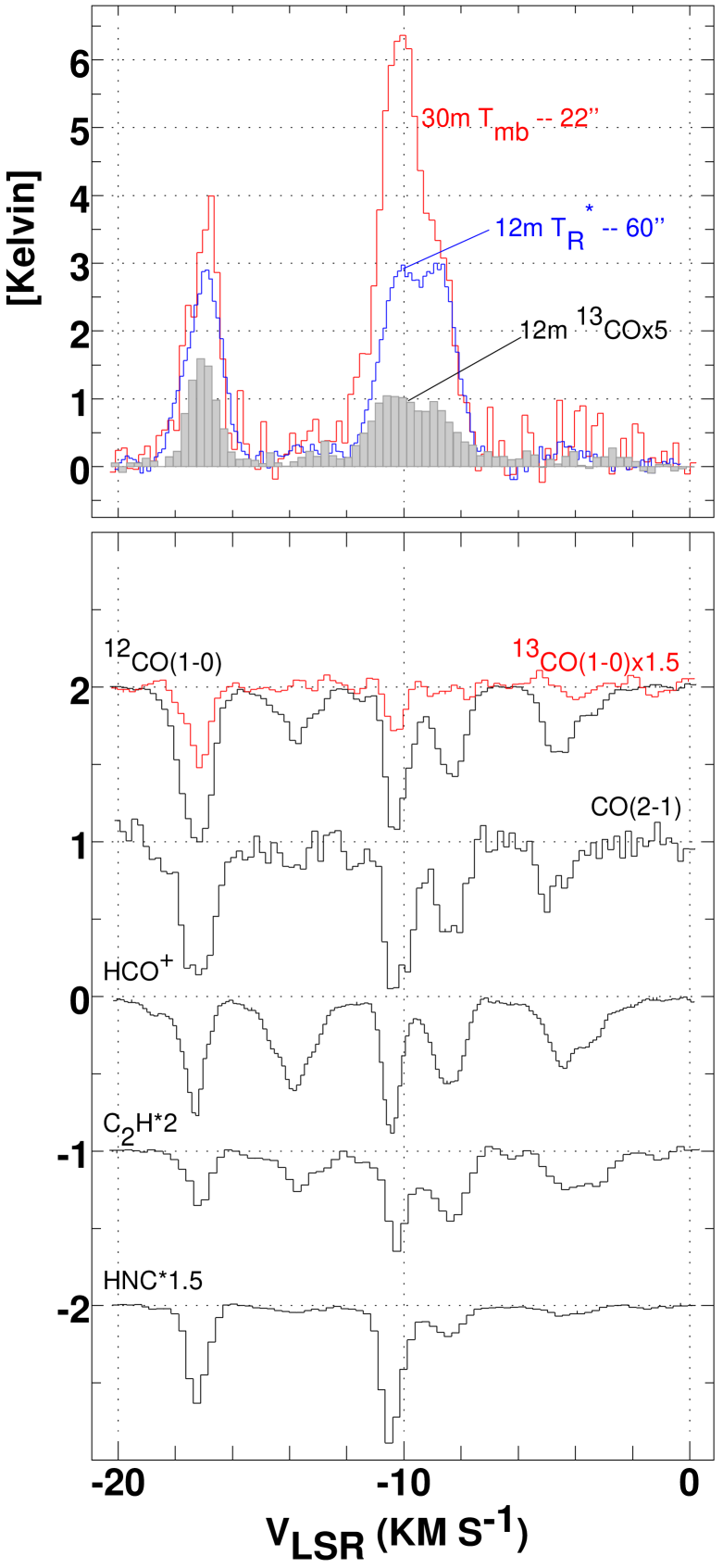
Figure 1: Emission and absorption spectra toward B0355+508 $aka$ NRAO150. Top panel: 1^′ HPBW J=1-0 ¹²CO and ¹³CO profiles from the former NRAO 12m telescope on a ${\rm T}_{\rm R}$^∗ brightness scale and the 22.5^′′-resolution IRAM 30m ¹²CO profile from the present work on a main-beam brightness temperature scale. Bottom: IRAM PdBI absorption profiles from various representative species. The profiles have been shifted vertically and scaled in some instances.

Unlike the vast majority of strong radio continuum sources, no visual identification of the blazar NRAO150 (Pauliny-Toth et al. 1966) has yet been made. At $\alpha=3$h59m29.73s, $\delta=50$^o57^′50.2^′′ (J2000), NRAO150 is seen at low latitude in the outer Galaxy ($l,b=$150.3772^o, -1.6037^o), so the path through the galactic disk is long and there is a heavy accumulation of distributed diffuse/H I gas. Quite aside from any dense material which might intervene, the integrated H I emission of the nearest spectrum in the Leiden-Dwingeloo H I survey (Hartmann & Burton 1997) gives an optically-thin lower limit N(H I) $>7.5\times 10^{21}\leavevmode\nobreak\ \leavevmode\nobreak\ {\rm cm}^{-2}$ or $\mathrm{A_{v}}>4\,\mathrm{mag}$. There is an approximate 5 kpc path length from the Sun out to a galactocentric radius of 13 kpc where the neutral gas disk might end (assuming R_☉ = 8.5kpc). For a typical mean gas density of $1\leavevmode\nobreak\ {\rm cm}^{-3}$, this corresponds to N(H) $=10^{22}\leavevmode\nobreak\ \leavevmode\nobreak\ {\rm cm}^{-2}$ or $\mathrm{A_{v}}\approx 6\,\mathrm{mag}$.

The sightline also harbors denser H₂-bearing clouds as shown in Fig. 1. While the H I absorption spectrum is too heavily saturated to be revealing (Liszt & Lucas 1996), the CO and HCO⁺ absorption spectra reveal 5-6 absorption features at LSR velocities of $-17.5$, $-14$, $-10.5$, $-8.5$, $-4.5/-3.5\,\mathrm{km\,s^{-1}}$. All those absorption features have comparable N(HCO⁺) $\approx 1\times 10^{12}\,\mathrm{cm^{-2}}$ implying N(H) $\approx$ 2N(H₂) $\approx 2\times 10^{21}\,\mathrm{cm^{-2}}$ (Lucas & Liszt 1996; Liszt & Lucas 1996) or $\mathrm{A_{v}}\approx 1\,\mathrm{mag}$. Each cloud also has N(OH) comparable to that seen toward $\zeta$ Oph (ibid), the prototypical diffuse cloud sightline studied optically (Van Dishoeck & Black 1986) where the visual extinction is 1$\,\mathrm{mag}$. As in optically-studied diffuse clouds (Sonnentrucker et al. 2007; Burgh et al. 2007; Sheffer et al. 2007), we derived N(CO) $<10^{15}-10^{16}\,\mathrm{cm^{-2}}$ (Lucas & Liszt 1998). This implies that only a modest fraction of the expected free gas-phase carbon N(C) $\approx 1.6\times 10^{-4}$ N(H) $\approx 3\times 10^{17}\,\mathrm{cm^{-2}}$ (Sofia et al. 2004) is incorporated in CO, as in any cloud with A_V$\la 1$ mag.

We conclude that the molecular features seen toward NRAO150 are hosted in diffuse or marginally translucent gas, consistent with the weakness of emission spectra in species other than CO and H I. OH emission seen at 18^′ resolution is quite weak (0.01$\,\mathrm{K}$) and very broad, extending over $-35<v<0\,\mathrm{km\,s^{-1}}$ and individual cloud features cannot be discerned (Liszt & Lucas 1996). The only species seen in mm-wave emission beside CO is HCO⁺ which appeared very weakly (0.01-0.02$\,\mathrm{K}$) at $v=-9\,\mathrm{km\,s^{-1}}$ when averaged over a several arcminute region (Lucas & Liszt 1996).

The absorption features display a rich and varied chemistry, a small sample of which is illustrated in the spectra of the bottom panel of Fig. 1. They harbor a prominent complement of typically ubiquitous species such as CO, C₂H and C₃H₂ (Lucas & Liszt 2000) as well as OH. All of the clouds also have detectable absorption in HNC, although weakly at $-14\,\mathrm{km\,s^{-1}}$ and $-4.5/-3.5\,\mathrm{km\,s^{-1}}$. The yet-stronger HCN spectrum is heavily confused by hyperfine structure, see Liszt & Lucas (2001) for a survey discussion of the CN-bearing species. The features at $-17.5\,\mathrm{km\,s^{-1}}$ and $-10.5\,\mathrm{km\,s^{-1}}$ are more chemically complex, with much more readily detectable amounts of the CN-family and such sulfur-bearing species as CS, SO, H₂S and HCS⁺ (Liszt & Lucas 2002) or H₂CO and NH₃  (Nash 1990; Marscher et al. 1993; Liszt & Lucas 1995; Liszt et al. 2006).

The top panel of Fig. 1 shows 1^′ HPBW CO and ¹³CO J=1-0 emission spectra from the former NRAO KP 12m telescope, which we used (in conjunction with the absorption spectrum) to check the CO column density and excitation temperatures toward this and other sources (Liszt & Lucas 1998). The two rather chemically-different absorption line components at $-10.5$ and $-8.5\,\mathrm{km\,s^{-1}}$ are heavily blended at 1^′ resolution, unlike the clearly double structure of the CO and other absorption. This is atypical of our comparisons in many other lines of sight between the absorption spectra of different species and the CO emission profiles when the latter are so strong. It is also curious because, being chemically so different, it would seem reasonable to believe that the two kinematic components were unrelated physically along the line of sight. Alternatively, the $-10.5$ and $-8.5\,\mathrm{km\,s^{-1}}$ components could be related and mixed with or enveloped by warmer optically thin gas which fills in the emission spectrum at $-10\,\mathrm{km\,s^{-1}}$ but not the absorption. However, as will be shown here, the two features are indeed part of the same structure and disparity between the emission and absorption profiles arises solely as the result of beam-smearing at 1^′ resolution.

Table 1: Observation parameters. The projection center of all the data matches the position of NRAO150: $\alpha_{2000}=03^{h}59^{m}29.747^{s}$, $\delta_{2000}=50{}^{\circ}57^{\prime}50.16^{\prime\prime}$.

Molecule	Transition	Frequency	Instrument	Config.	Beam	PA	Vel. Resol.	Int. Time	$T_{\mathrm{sys}}$	Noisea	Obs. date
		GHz			arcsec	∘	$\,\mathrm{km\,s^{-1}}$	hours	K	K
12CO	$J$=1–0	115.271202	PdBI	D	$6.0\times 5.5$	82	0.2	3.3/12.5	230	0.20	Jul. 2005
12CO	$J$=1–0	115.271202	PdBI	C	$2.7\times 2.5$	12	0.2	7.0/12.0	230	0.52	Dec. 2005

^a The noise values quoted here are the noises at the mosaic phase center (Mosaic noise is inhomogeneous due to primary beam correction; it steeply increases at the mosaic edges).

Molecule	Transition	Frequency	Instrument	# Pix.	$F_{\mathrm{eff}}$	$B_{\mathrm{eff}}$	Resol.	Resol.	Int. Timea	$T_{\mathrm{sys}}$	Noiseb	Obs. date
		GHz					arcsec	$\,\mathrm{km\,s^{-1}}$	hours	K	K
12CO	$J$=1–0	115.271202	30m/AB100	2	0.95	0.75	22.5	0.20	2.4/3.6	240	0.26	Sep. 2005
12CO	$J$=2–1	230.538000	30m/AB230	2	0.91	0.52	22.5	0.20	2.4/3.6	320	0.16	Sep. 2005

^a Two values are given for the integration time: the on-source time and the telescope time.
^b Noise values estimated at the position of NRAO150.

Several of the features (at $-14$ and $-4.5/-3.5\,\mathrm{km\,s^{-1}}$) seen so strongly in CO and HCO⁺ absorption are almost absent in CO emission. Can these particular clouds really be dense enough to form HCO⁺ and the hydrocarbons C₂H and C₃H₂, along with relatively small amounts of HNC and HCN, but not dense enough to form detectable amounts of NH₃  or H₂CO (Liszt et al. 2006) or even dense enough to excite CO to detectable levels? The clouds at $-14$, $-4.5/-3.5\,\mathrm{km\,s^{-1}}$ which are so weak in CO emission have non-negligible J=1-0 optical depths 0.3 - 0.6 in ¹²CO, implying that their excitation temperatures are less than 1$\,\mathrm{K}$ above the cosmic microwave background. Comparably low excitation temperatures have recently been found to be common in CO seen in the $uv$ absorption spectra of bright stars when N(CO) $<2\times 10^{15}\leavevmode\nobreak\ \leavevmode\nobreak\ {\rm cm}^{-2}$ and N(H₂) $<5\times 10^{20}\leavevmode\nobreak\ \leavevmode\nobreak\ {\rm cm}^{-2}$ (Burgh et al. 2007; Sonnentrucker et al. 2007), the latter equivalent to N(HCO⁺) $\la 10^{12}\leavevmode\nobreak\ \leavevmode\nobreak\ {\rm cm}^{-2}$. Although one might also wonder if such H₂-bearing, CO-silent clouds are just very cold, perhaps part of the dark molecular baryonic matter which has been hypothesized to exist in the disks of galaxies (Pfenniger et al. 1994), the H₂ seen in $uv$ absorption along comparable sightlines hosting weakly-excited CO indicates kinetic temperatures of 40-80$\,\mathrm{K}$ and the kinetic temperature inferred from C₂ is only slightly lower (ibid).

In summary, the line of sight towards NRAO150 is very heavily extincted, having an exceptionally large column of intervening neutral gas compared to other sources we have studied. Nonetheless, the occulting material is not manifestly dark in a local sense. About 6$\,\mathrm{mag}$ of visual extinction comes from low density (1$\,\mathrm{cm^{-3}}$) gas along the 4-5kpc length of the sightline. Comparable intervening column density of H-nuclei comes from 5-6 diffuse clouds ($\mathrm{A_{v}}\sim 1\,\mathrm{mag}$ each), which display a surprisingly complex chemistry relative to their modest inferred column density.

In an attempt to characterize more fully the nature of the host gas clouds, we undertook to map CO emission around the NRAO150 sightline. However, targeting NRAO150 involves making one serious tradeoff: in return for access to kinematic complexity along with the ability to map several strongly-absorbing clouds simultaneously and the chance to address various puzzles raised by our previous observations, we forfeit precise knowledge of the distances of the intervening clouds. Only an angular scale may readily be attached to our present conclusions, a fact typical of observations in the galactic plane. For reference, we note that the line of sight velocity gradient in the disk, assuming a flat rotation curve with $R_{0}=8.5\rm kpc$ and a rotation velocity of $220\,\mathrm{km\,s^{-1}}$ implies 1) a line of sight distance of 2.5kpc for a velocity of $-20\,\mathrm{km\,s^{-1}}$ (i.e. at the blue edge of our strong absorption features) and 2) a distance uncertainty of $\pm 0.75\rm kpc$ associated with the typical cloud-cloud velocity dispersion of 6$\,\mathrm{km\,s^{-1}}$. At a distance of 1kpc, 1^′ corresponds to 0.3pc.

3 Observations and data reduction

3.1 Observations

We used the IRAM Plateau de Bure Interferometer (PdBI) to achieve higher spatial resolution in mapping CO emission from the gas toward NRAO150. However, an interferometer filters out low spatial frequencies of the source distribution and to supply the missing but much-needed information we observed the same region of the sky with the IRAM-30m telescope. In this Section we describe in detail how these observations were taken, reduced and merged to form the on-the-fly (OTF) and hybrid synthesis results.

3.1.1 IRAM Plateau de Bure Interferometer observations

PdBI observations dedicated to this project were carried out with 5 antennae in the CD configuration (baseline lengths from 24$\,\mathrm{m}$ to 229$\,\mathrm{m}$) from July to December 2005. Three correlator bands of 20 MHz were concatenated around the ¹²CO $J$=1–0 frequency to cover a $\sim 50\,\mathrm{km\,s^{-1}}$ bandwidth at a resolution of $\sim 0.1\,\mathrm{km\,s^{-1}}$. Two additional correlator bands of 320 MHz were used to measure the 2.6$\,\mathrm{mm}$ continuum over the 580$\,\mathrm{MHz}$ instantaneous IF-bandwidth available with this generation of receivers.

We observed a seven–field mosaic. The mosaic was centered on the position of NRAO150 and the field positions followed a compact hexagonal pattern to ensure Nyquist sampling in all directions. This mosaic was observed for about 24 hours of telescope time with 4 to 6 antennas. Taking into account the time for calibration and after filtering out data with rms tracking error larger than $1^{\prime\prime}$ (computed over the scan length), this translated into on–source integration time of useful data of 3.3 hours in the D configuration and 7 hours in the C configuration for a full 6-antenna array. Typical 2.6$\,\mathrm{mm}$ resolution is $5.8^{\prime\prime}$ in the D configuration and $2.6^{\prime\prime}$ in the C configuration.

3.1.2 IRAM-30m singledish observations

Table 2: NRAO150 flux in Jy.

Date	2.6$\,\mathrm{mm}$	1.3$\,\mathrm{mm}$
17.07.2005	2.8	1.6
28.07.2005	2.8	1.6
01.08.2005	2.9	1.7
12.12.2005	2.4	1.4

The ¹²CO $J$=1–0 and $J$=2–1 lines were observed simultaneously during about 4 hours of good summer weather ($\sim 4\,\mathrm{mm}$ of water vapor) in September 2005. The four available single-side band mixers were used (two per frequencies: AB100 and AB230) in the OTF observing mode to map a field-of-view of $220^{\prime\prime}\times 220^{\prime\prime}$ centered on the position of NRAO150. The dump time was 1 second and the scanning speed $\sim 3^{\prime\prime}/$sec. The field-of-view was covered twice by raster-scanning along the RA axis and once by scanning along the Declination axis. The HPBW of the telescope for the J=1-0 line is 22^′′ and the rasters were separated by $10^{\prime\prime}$, providing Nyquist sampling at 2.6$\,\mathrm{mm}$ but undersampling at 1.3$\,\mathrm{mm}$. We estimate the 30m position accuracy to be $\sim 2^{\prime\prime}$.

We used the ON-OFF switching mode and separately observed the reference position at $(+400^{\prime\prime},0^{\prime\prime})$ during 62 minutes using frequency switching mode with a frequency throw of 7.7$\,\mathrm{MHz}$ (optimal to suppress standing waves) to check for the presence of signal. Emission was detected at $\lambda$2.6$\,\mathrm{mm}$ and later added back into the on-the-fly emission profiles.

3.2 Data reduction

The data processing was done with the GILDAS software suite (Pety 2005).

3.2.1 Singledish calibration

The IRAM-30m data were processed inside GILDAS/CLASS software. They were first calibrated to the $T_{\mathrm{A}}^{*}$ scale using the chopper wheel method (Penzias & Burrus 1973), and finally converted to main beam temperatures (${\rm T}_{\rm mb}$) using the forward and main beam efficiencies ($F_{\mathrm{eff}}$ & $B_{\mathrm{eff}}$) displayed in Table 1. The resulting amplitude accuracy is $\sim$ 10%. The line window was fixed between $-25$ and $10\,\mathrm{km\,s^{-1}}$ and a second order baseline was subtracted from each on-the-fly spectrum. The off-position frequency-switched spectrum was fitted by a combination of Gaussians after baseline subtraction and this fit was then added to every on-the-fly spectrum.

To compensate for the presence of absorption in the OTF-data near the continuum background source, the absorption spectra measured several years ago at PdBI (Liszt & Lucas 1998) were scaled to the flux of NRAO150 at the observation date (Table 2 here), converted to main beam temperature, convolved by a Gaussian whose full width at half maximum corresponds to the natural resolution of the 30m at the observing frequency, and (at last) subtracted from each on-the-fly spectrum. The resulting spectra were finally gridded through convolution by a Gaussian. The ¹²CO $J$=2–1 data were gridded at the same spatial resolution (e.g. $22.5^{\prime\prime}$) as the ¹²CO $J$=1–0 data on account of the observational undersampling at the higher frequency.

3.2.2 Inteferometric calibration

The first steps of the standard calibration methods implemented inside the GILDAS/CLIC software were used for the PdBI data. The radio-frequency bandpass was calibrated using observations of 3C354.4 leading to an excellent bandpass accuracy because its 2.6$\,\mathrm{mm}$ flux was larger than 20 Jy at the epochs of the observations. The flux of NRAO150 was determined against the primary flux calibrator used at PdBI, i.e. MWC349. The resulting flux accuracy is $\sim$ 15%.

We then took advantage of the presence of the strong NRAO150 point source continuum (Table 2) to get a very accurate phase and amplitude calibration. $uv$ tables for the 2.6$\,\mathrm{mm}$ continuum and the ¹²CO $J$=1–0 were created and time dependencies of the phase and amplitude of the continuum were self-calibrated per baseline through the use of the GILDAS/UV_GAIN task. The temporal phase and amplitude gain derived during this self-calibration step were applied to the ¹²CO $J$=1–0 $uv$-tables through the use of the GILDAS/UV_CAL task. Those last two steps were done for each individual mosaic field taking into account that the flux of NRAO150 is attenuated differently by the interferometer primary beam depending on the field position. They were also done on each individual observation session to take into account the temporal variations of the NRAO150 flux. Finally, the ¹²CO $J$=1–0 absorption spectrum was added back to the data after rescaling to the flux of NRAO150 at the epoch of observation.

3.2.3 Short-spacing processing, imaging and deconvolution

Following Gueth et al. (1996), the GILDAS/MAPPING software and the singledish map from the IRAM-30m were used to recreate the short-spacing visibilities not sampled at the Plateau de Bure. These were then merged with the interferometric observations. Each mosaic field was then imaged and a dirty mosaic was built combining those fields in the following optimal way in terms of signal–to–noise ratio (Gueth 2001)

$$J(\alpha,\delta)=\sum\nolimits_{i}\frac{B_{i}(\alpha,\delta)}{\sigma_{i}^{2}}\,F_{i}(\alpha,\delta)\left/\displaystyle\sum\nolimits_{i}\frac{B_{i}(\alpha,\delta)^{2}}{\sigma_{i}^{2}}.\right.$$

In this equation, $J(\alpha,\delta)$ is the brightness distribution in the dirty mosaic image, $B_{i}$ are the response functions of the primary antenna beams, $F_{i}$ are the brightness distributions of the individual dirty maps and $\sigma_{i}$ are the corresponding noise values. As may be seen in this equation, the dirty intensity distribution is corrected for primary beam attenuation, which make the noise level spatially inhomogeneous. In particular, noise strongly increases near the edges of the field of view. To limit this effect, both the primary beams used in the above formula and the resulting dirty mosaics are truncated. The standard level of truncation is set at 20% of the maximum in MAPPING. The dirty image was deconvolved using the standard Högbom CLEAN algorithm. The resulting data cube was then scaled from Jy/beam to ${\rm T}_{\rm mb}$ temperature scale using the synthesized beam size (see Table 1).

Although we also obtained data in the C configuration of PdBI, we present here only the combination of the more compact D configuration with the IRAM-30m singledish data. Indeed, we were not able to correctly deconvolve the combination of C + D configuration and singledish data. We guess that this is due to the too low signal-to-noise ratio of the C configuration data.

3.3 Field of view and finally-achieved resolution

The resolution of the shown OTF singledish maps is 22.5^′′ both for the ¹²CO J=1-0 and J=2-1 lines. As noted in Table 1, the spatial resolution of the hybrid synthesis results shown here (using the D-array data) is 5.8^′′ ($6.0^{\prime\prime}\times 5.5^{\prime\prime}$).

The 220^′′ extent and 90^′′ diameter of the OTF and hybrid maps correspond in angle to the HPBW of typically-illuminated telescopes (HPBW = $1.2\lambda$/D) of diameter D = 2.9m and 7.2m in the J=1-0 line and the 5.8^′′ synthesis beam corresponds to D = 109m.

3.4 Relative intensities

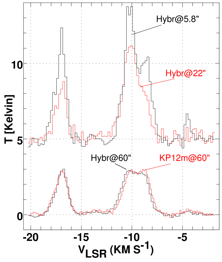
Figure 2: Evolution of J=1-0 ¹²CO brightness with angular resolution. At bottom, the profile from the former NRAO 12m telescope is compared with hybrid synthesis data convolved to 1^′ HPBW. At top the hybrid data centered on the continuum source are displayed at full (5.8^′′) and 30m (22.5^′′) resolution. Note that the hybrid synthesis profile much more closely resembles the absorption spectra shown in Fig. 1 at bottom.

The validity of the discussion depends on the consistency of the intensity calibration across several instruments and over a wide variety of spatial scales. For the ${\rm T}_{\rm R}$^∗ scale employed at the 12m telescope, the antenna temperature is standardly scaled up by 1/0.85 representing the fraction of the forward response subtended by the Moon. To put the data on its standard main-beam scale ${\rm T}_{\rm mb}$, IRAM-30m antenna temperatures are scaled up by 1/0.75 (see Table 1 here) representing the fraction of the forward response in the main beam.

To make the point that these intensity scales are consistent, Fig. 1 and 2 compare the profiles toward NRAO150 at the same angular resolution from different instruments: 1) 22.5^′′ spectra from the IRAM-30m and the smoothed synthesis data and 2) 60^′′ spectra from the Kitt Peak 12m and the smoothed synthesis data. The thin line (red) spectrum in the upper part of Fig. 2 displays the convolution of the hybrid synthesis data to the resolution of the IRAM-30m telescope. The agreement with the IRAM-30m spectrum shown in the top panel of Fig. 1 demonstrates the reliability of the algorithm used to merge the singledish and interferometric data. At bottom in Fig. 2, we also show the result of convolving the hybrid synthesis data to the 60^′′ resolution of the 12m telescope without any further amplitude rescaling. However coincindentally, the convolved hybrid synthesis data reproduce the 12m telescope integrated intensity to within 4 percent in either strong feature as well as the detailed profiles themselves (although there is a very slight velocity shift in the gas around $-10\,\mathrm{km\,s^{-1}}$). Therefore we are confident that the very strong lines seen here at high resolution, 12-13$\,\mathrm{K}$, are not artifacts of instrumental calibration.

Finally, the 22.5^′′ resolution emission profile from the IRAM-30m in the top panel of Fig. 1 is more than twice as strong as that from the 12m (not just 0.85/0.75) and that from the hybrid synthesis at the top of Fig. 2 is 30% stronger still. This profile evolution arises from increased spatial resolution.

4 New Observational Results

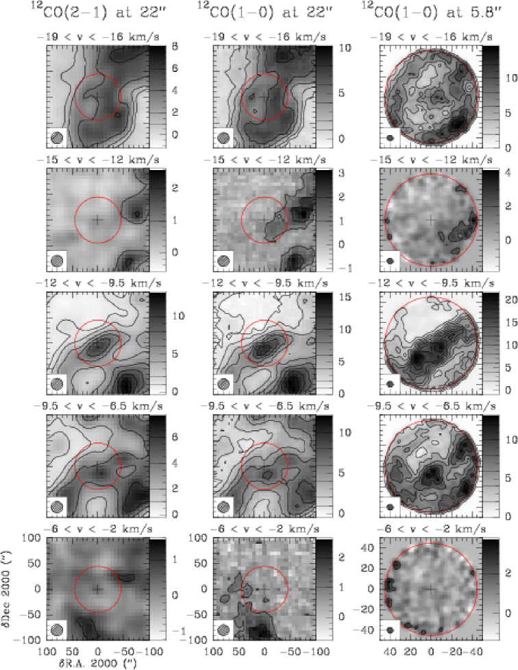
Figure 3: Summary of mapping information of the diffuse gas around NRAO150. Each panel shows the ¹²CO emission integrated over the velocity range of one absorption feature visible in Fig. 1, i.e. from top to bottom the $-17.5$, $-14$, $-10.5$, $-8.5\,\mathrm{km\,s^{-1}}$ and, combined, the $-4.5$ and $-3.5\,\mathrm{km\,s^{-1}}$ features. The position of NRAO150 is marked by a cross at the map center. The left and middle columns show respectively the ¹²CO $J$=2–1 and $J$=1–0 emission observed with the 30m singledish antenna while the right column shows the ¹²CO $J$=1–0 emission at higher resolution from hybrid synthesis data (i.e. the combination of the 30m and PdBI instruments). The 30m ¹²CO $J$=2–1 map has been smoothed to $22.5\mbox{${}^{\prime\prime}$}$. The field of view of the hybrid synthesis maps is about half that of the singledish data: As a guide, the red circle has the same 45^′′-radius in all panels. The resolution of the hybrid synthesis data (5.8^′′) is almost 4 times better than that of the singledish data, 22.5^′′. Contour levels are spaced by 2 $\,\mathrm{K\,km\,s^{-1}}$, but for the first contour for the singledish maps which is at 1$\,\mathrm{K\,km\,s^{-1}}$. Contour levels are shown on the intensity look-up tables.

4.1 Emission spectra toward NRAO150

The upper part of the top panel of Fig. 1 compares the 22.5^′′ resolution IRAM-30m spectrum from the present work with its 1^′ KP counterpart toward the continuum source. To the extent that the $-17.5$ and $-8.5\,\mathrm{km\,s^{-1}}$ emission features resemble themselves as the linear resolution increases by a factor of 3, it might be inferred that the CO emission shows little structure on sub-arcminute scales. Conversely, the brightness increases by almost a factor 2 at $-10.5\,\mathrm{km\,s^{-1}}$, indicating stronger sub-structure.

While the 22.5^′′ resolution IRAM-30m spectrum resolves some but not all of the disparity between the 1^′ KP CO emission profile and the distinct doubling of the absorption components at $-10.5$ and $-8.5\,\mathrm{km\,s^{-1}}$, the 6^′′ on-source hybrid synthesis profile in Fig. 2 much more strongly resembles the absorption profile around $-10\,\mathrm{km\,s^{-1}}$. So, after much work, we are finally able to say that the disparity between the 1^′ KP12m profile and the absorption is due to spatial gradients and the coincidental positioning of the continuum source with respect to the foreground gas.

4.2 Summary maps of emission integrated over each absorption feature

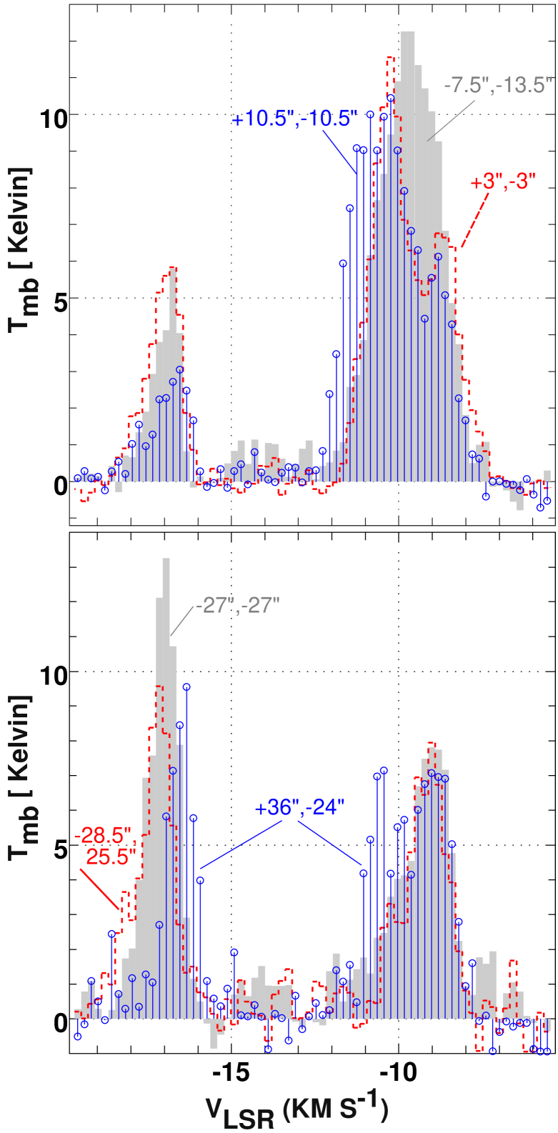
Figure 4: Hybrid synthesis CO J=1-0 (5.8^′′ resolution) profiles at selected locations of particularly strong emission. Top: Profiles selected from a map of peak emission near $-10\,\mathrm{km\,s^{-1}}$. Bottom: Selected from a map of peak emission near $-17\,\mathrm{km\,s^{-1}}$. Profiles are labelled by their displacement $(\Delta\alpha,\Delta\delta)$ in arcseconds relative to the continuum source.

To understand the overall behavior, Fig. 3 shows summary maps integrated over five velocity ranges corresponding to the features seen in absorption.

The feature at $-17.5\,\mathrm{km\,s^{-1}}$ is present over the full extent of the region mapped and/or synthesized but with substantial intensity contrast, of order 4:1 even in the middle, top panel of Fig. 3. At 6^′′ resolution at right, there is emission toward and around the continuum and a somewhat higher contrast, from a low of 2.1$\,\mathrm{K\,km\,s^{-1}}$ (just north of NRAO150) to 14.5$\,\mathrm{K\,km\,s^{-1}}$ near the southwest rim of the synthesized region.

The weak emission features at $-14$ and near $-4\,\mathrm{km\,s^{-1}}$ occupy relatively small fractions at the edges of the area mapped at 5.8^′′ resolution in Fig. 3 and approach but do not extend across the continuum position. Stronger emission exists within the IRAM-30m map outside the hybrid synthesis field of view but the beams employed here are mostly unfilled when pointed on-source: there are no isolated hot spots within the synthesized region which were lost to beam dilution in the singledish data. We can thus deduce that any difficulty in detecting emission around NRAO150 in these features is purely an excitation effect, because the optical depths measured from the absorption profiles are of order 0.5 in either case.

As suggested by the comparison between the 30m and 12m profiles in Fig. 1, the sharpest spatial structure near the continuum source occurs in the panels centered at $-10.5\,\mathrm{km\,s^{-1}}$ in Fig. 3. The ridge of emission which passes near NRAO150 appears to have been at most barely resolved by the 30m telescope at $-10.5\,\mathrm{km\,s^{-1}}$, while a very similar structure at $-8.5\,\mathrm{km\,s^{-1}}$ in the OTF maps is more spatially extended and better resolved.

Perhaps the clearest result in Fig. 3 is the transverse resolution and isolation of the ridge at $-10.5\,\mathrm{km\,s^{-1}}$ near NRAO150 in the hybrid synthesis data at right, and, to a slightly lesser extent, at $-8.5\,\mathrm{km\,s^{-1}}$ as well. Over the region of the synthesis the integrated intensity contrast is high, above 16:1, but the emission does not break up into a patchwork of unresolved and/or isolated bright and dark regions. As discussed below, uniformity is to some extent an artifact of the high optical depth in the middle of the ridge, enhanced by integration over velocity which suppresses spatial structure even at the northern edge of the ridge where (see Sect 4.5 and Fig. 7) it is heavily kinematically structured.

Taken together, similarity in the third and fourth row of Fig. 3 strongly suggests that the features seen at $-10.5$ and $-8.5\,\mathrm{km\,s^{-1}}$ are actually part of the same structure, no matter that they are distinct in absorption, separated in emission at sufficiently high spatial resolution and substantially different in the richness of their chemistry.

4.3 Channel maps at 1 km s^-1 resolution

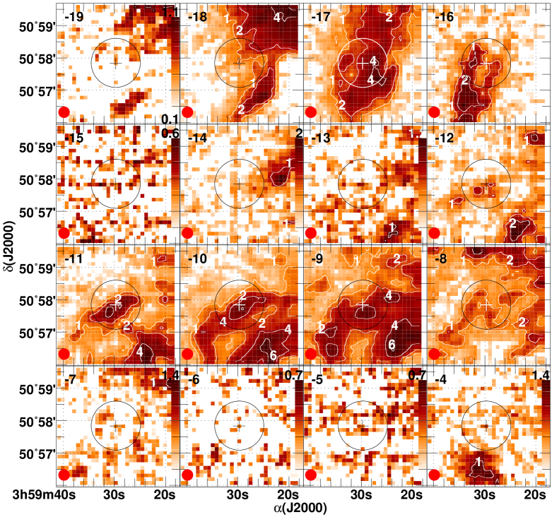
Figure 10: Finer-scale singledish maps of integrated ¹²CO brightness. The 30m on-the-fly mapping observations used as short-spacing input to the hybrid synthesis are summed over the 5-channel (1.015 $\,\mathrm{km\,s^{-1}}$) intervals most closely centered about the velocity indicated at the upper left in each panel and the integrals are scaled down by 1/1.015 to reflect mean brightness over a 1 $\,\mathrm{km\,s^{-1}}$-wide interval. Contours are shown at levels 1,2,4,6,8, 10$\,\mathrm{K\,km\,s^{-1}}$. The position of NRAO150 is marked by a cross at the map center and the region synthesized is shown as a circle. Note the velocity gradient in the $-17\,\mathrm{km\,s^{-1}}$ feature across the position of NRAO150. The 22.5^′′ HPBW is shown inset at the lower left in each panel.

Fig. 10 and 11 (available on-line) show a series of channel maps with a resolution of $1\,\mathrm{km\,s^{-1}}$ for the IRAM-30m and PdBI data. The weakly-emitting gas at $-14$, $-4.5$ and/or $-3.5\,\mathrm{km\,s^{-1}}$ is only marginally seen near the field center and an East-West velocity gradient across NRAO150 is resolved in the $-17.5\,\mathrm{km\,s^{-1}}$ gas with more positive velocities seen to the South and East. The blue wing of emission at $-11\,\mathrm{km\,s^{-1}}$ is disposed on either side of the source (somewhat filling in the gaps of the distribution at $-10\,\mathrm{km\,s^{-1}}$).

Increasing the velocity discrimination to this extent still does not show substantially smaller scale spatial structure in the emission pattern with the possible exception of the panel at $-8\,\mathrm{km\,s^{-1}}$, in the near wing of the strong emission feature. The high optical depths measured in the $-17.5\,\mathrm{km\,s^{-1}}$ feature and in the components at $-10.5$ and $-8.5\,\mathrm{km\,s^{-1}}$ may impede viewing such structure: No matter how sharp the actual internal structure, it can only be seen if the line of sight penetrates deeply enough to probe it. This behavior is illustrated in greatest detail in Fig. 7 and discussed in Sect. 4.5.

4.4 Bright spots, area filling factors and spatial statistics

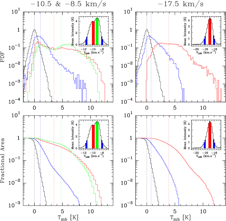
Figure 5: Top: Probability distribution function of the line brightness in the hybrid synthesis, normalized to unit area. Bottom: Fractional area (cumulative distribution) of pixels whose line brightness is higher than the value given on the abscissa. Right: for the component at $-17.5\,\mathrm{km\,s^{-1}}$. Left: for the $-10.5$ and $-8.5\,\mathrm{km\,s^{-1}}$ components. The histograms have been computed in the line wings (blue curves), the line cores (red and green curves) and baseline devoid of signal (black curve). For reference, the averaged spectra are shown as inset with the same color scheme. The vertical dotted lines display the line brightness medians.

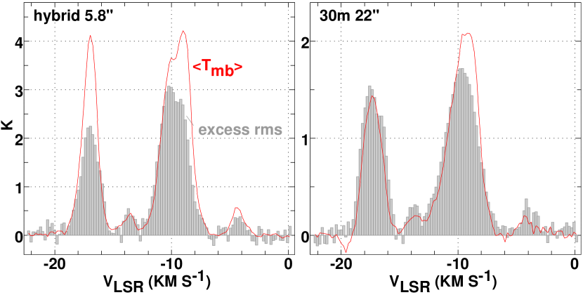
Figure 6: Mean profiles ($<\mbox{${\rm T}_{\rm mb}$}>$, red lines) and rms spatial brightness fluctuation in excess of the random noise rms ($\sqrt{\mbox{RMS}(\mbox{${\rm T}_{\rm mb}$})^{2}-\mbox{RMS(noise)}^{2}}$, shaded histrogram). Left: For the 5.8^′′ resolution hybrid synthesis data (random noise: 0.47$\,\mathrm{K}$). Right: For the 30m OTF mapping data at $22.5^{\prime\prime}$ resolution (random noise: 0.33$\,\mathrm{K}$).

Fig. 4 displays profiles selected from hybrid maps of peak brightness in the gas around $-10\,\mathrm{km\,s^{-1}}$ (see the top panel) and at $-17\,\mathrm{km\,s^{-1}}$. There are some very strong lines in the region of the synthesis, ${\rm T}_{\rm mb}$= 12-13$\,\mathrm{K}$, which was hardly expected on the basis of the 3$\,\mathrm{K}$ lines in the emission spectra at 1^′ in Fig. 1. As indicated by the spatial offsets labelling the spectra in the top panel of Fig. 4, such unusually strong lines exist very close to NRAO150, i.e. just outside the on-source synthesized beam but still inside the on-source 30m beam. These lines imply CO J=1-0 excitation temperatures of at least 16-17$\,\mathrm{K}$, far stronger than is typical of very dark clouds where $\mbox{${\rm T}_{\rm K}$}<10\,\mathrm{K}$. Perhaps an analogous surprise was that of Heithausen (2004), whereby a very weak (0.2$\,\mathrm{K}$) ¹²CO J=1-0 line inadvertently seen at the 30m was subsequently found in high-resolution PdBI maps to consist of a much brighter, unresolved spicule.

The beam efficiency needed to convert observed antenna temperatures to actual sky brightness has two aspects; the extent of the sky distribution – which antenna lobes are subtended – and the degree of uniformity or area filling factor within that extent. In fact there is a high degree of heterogeneity on all the scales which are resolved in the present dataset. Fig. 5 expresses this fact quantitatively by showing the fractional area occupied by emission at all observed levels of brightness. We defined a circle of radius 45^′′ within the hybrid synthesis map and constructed histograms of the brightness distribution for all included pixels over various channel ranges. At left in Fig. 5 are the differential and cumulative distributions for the near wings and cores of the $-10.5$ and $-8.5\,\mathrm{km\,s^{-1}}$ features and at right are those for the $-17.5\,\mathrm{km\,s^{-1}}$ feature.

Cartoons inset in each panel show the profile intervals which were employed, superposed on the mean profile formed over the region. These mean spectra have brightnesses of 3.6 - 4.2$\,\mathrm{K}$ in the line cores and approximately 1$\,\mathrm{K}$ in the selected regions of the line wings. Noise statistics are not necessarily the same for channels with and without emission (after deconvolution) but for reference we constructed similar histograms for channels in emission-free baseline regions of the spectrum (as shown). 90% of the noise occurs below 0.7$\,\mathrm{K}$ and 95% below 1$\,\mathrm{K}$; the nominal single-channel rms noise averaged over the region of the synthesis is 0.47$\,\mathrm{K}$ in emission-free baseline regions of the spectrum.

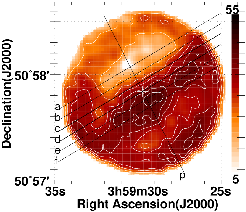
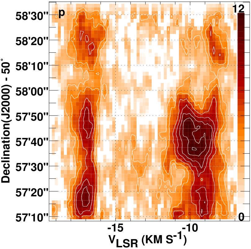
Figure 7: Position–velocity diagrams across and along the main trunk feature at a position angle of $-50$^o. Top, left: Integrated intensity map of 5.8^′′-resolution hybrid synthesis data summed over the disjoint velocity ranges $[-19..-15]\,\mathrm{km\,s^{-1}}$ and $[-12.5..-7.5]\,\mathrm{km\,s^{-1}}$. Contours are shown at levels 5,10,15,..35$\,\mathrm{K}$$\,\mathrm{km\,s^{-1}}$. The position of NRAO150 is marked by a cross at the map center. Bottom, left: A position–velocity diagram along the perpendicular strip p through the position of NRAO150 at 5.8^′′ resolution. Contours are shown at levels 0.5,1,2,4,6,8,10,12$\,\mathrm{K}$. Top, right: Longer position–velocity diagram at 22.5^′′ resolution straddling strip d, made from 30m data. Contours are shown at levels 0.5,1,2,4,6,8,10,12 $\,\mathrm{K\,km\,s^{-1}}$. Bottom, right: Position–velocity maps at 5.8^′′ resolution along strips a-f. Coordinates are displacement in right ascension relative to NRAO150. Strip d precisely crosses the continuum source.

Pixel histograms for the line cores are strongly populated up to 7-8$\,\mathrm{K}$ and have tails extending to 10-13$\,\mathrm{K}$. Even pixels in the 1$\,\mathrm{K}$ line wings have higher-intensity tails extending up to 6-7$\,\mathrm{K}$, reflecting substantial local excursions of the line centroids (see Fig. 4 and 7). Such wide distribution of intensity ensures that fluctuations are a significant fraction of the mean. A plot of the true spatial rms variation in each channel, i.e. the rms variation above and beyond that attributable to radiometer noise (e.g. 0.47$\,\mathrm{K}$ averaged over the field of the the hybrid synthesis and 0.33$\,\mathrm{K}$ in the 30m OTF data), calculated as the square root of the quadrature difference between the total and noise rms, is shown in Fig. 6.

For the larger $220^{\prime\prime}\times 220^{\prime\prime}$ region of the 30m OTF data this excess rms is closely equal to the mean across the entire spectrum, except between $-9$ and $-10\,\mathrm{km\,s^{-1}}$ where the mean exceeds the rms by 20-30%. For this gas, increasing the spatial resolution to 5.8^′′ yields only a small increase in the ratio of mean and excess rms brightness. By contrast, the character of the comparison changes drastically for the $-17.5$ feature at higher resolution, where the excess rms changes from 100% to only 50% of the mean at the line core when going from the IRAM-30m to the synthesis data.

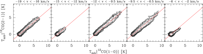
Figure 8: Joint distributions of the emission of ¹²CO $J$=2–1 and $J$=1–0. The value at a given position of these joint histograms is the number of pixels of the input images whose intensities lye in the respective vertical and horizontal bins. Contour levels are set to 1, 2, 4, 8, 16, … 512 points per pixel. The joint distributions have been computed and plotted for each velocity components. A (red) line of slope of 0.725 is shown for reference. Only the emission around $v=-4\,\mathrm{km\,s^{-1}}$ in the rightmost panel departs noticeably from the mean behavior.

The actual pixel statistics of the brightness distributions are given in Fig. 6 but fluctuations equal to the mean are most commonly recognized as characteristic of Poisson statistics, which would be observed from a macroscopically transparent ensemble of statistically independent clumps. Conversely, large ratios of mean to rms brightness might imply that the innate structure has been completely spatially resolved. However the situation is both more complex and more interesting, because the synthesis data also resolves the kinematic substructure of the features in ways which are not reflected in this discussion.

4.5 A detailed view of line kinematics

The full extent of the variation in CO emission can only be revealed by examining the data at the highest available spectral resolution. Fig. 7 explores the kinematics on a series of tracks along and across the rather linear structure seen around $-10\,\mathrm{km\,s^{-1}}$. The tracks, shown overlaid on an integrated intensity map at top left in the Figure, are separated vertically (in Declination) by 4 pixels or 6^′′ which is very nearly one synthesized HPBW. Spectra along the transverse track p are shown at bottom left, where the vertical scale is elongated compared to the others at right in the figure. At top right is a larger-scale diagram along track d using 30m data and below it are shown the hybrid synthesis data along tracks a-f. Comparing the track at the top right in Fig. 7 with those below is a striking deconstruction of the singledish lower-resolution data into its interferometric high-resolution components.

The simple, essentially featureless East-West velocity gradient in the $-17.5\,\mathrm{km\,s^{-1}}$ gas at top right in Fig. 7 is manifest along strips a-e but the manner in which the velocity change occurs is striking at high resolution, with abrupt reversals and line-splittings; it is zig-zag and meandering rather than smooth. The same is true for the emission around -10$\,\mathrm{km\,s^{-1}}$, in those strips (a-e) mostly above the mid-line of the long trunk. Along track f, the line profile over the complex is filled in by stronger and presumably very opaque emission seen in the profile labelled (-7.5^′′,-13.5^′′) in Fig. 4. We hypothesize that the line of sight penetrates deeply into the medium around $-10\,\mathrm{km\,s^{-1}}$ at the edge of the trunk along tracks a-d, and that kinematic details largely disappear along the tracks e-f as the medium becomes fully opaque in a macroscopic sense; note the excursions in the line wing at $v<-11\,\mathrm{km\,s^{-1}}$ even along tracks e-f. The combination of beam-smearing and the strength of emission just south of NRAO150 combine in on-source singledish data to obscure the double-lined structure apparent in absorption or at high spatial resolution.

4.6 Rotational excitation

Insight into the nature of the host gas is hindered by the unavailability of high-resolution observations other than of ¹²CO and the lack of high spatial resolution even in the J=2-1 line. However, in diffuse gas where the CO/H₂ ratio is small and sharply variable, where the ¹²CO/¹³CO ratio can be strongly altered by fractionation, and where the rotational excitation is sub-thermal (Liszt & Lucas 1998; Sonnentrucker et al. 2007; Burgh et al. 2007; Sheffer et al. 2007; Liszt 2007a), many of the underpinnings of typical analysis of CO profiles must be questioned in any case.

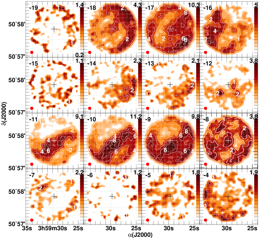
Figure 11: Finer-scale hybrid synthesis maps of integrated ¹²CO brightness. The 5.8^′′ hybrid synthesis profiles are summed over the 5-channel (1.05 $\,\mathrm{km\,s^{-1}}$) intervals most closely centered about the velocity indicated at the upper left in each panel and the integrals are scaled by 1/1.05 to reflect mean brightness over a 1$\,\mathrm{km\,s^{-1}}$-wide interval. Contours are shown at levels 1,2,4,6 and 8$\,\mathrm{K\,km\,s^{-1}}$. The position of NRAO150 is marked by a cross at the map center. The 5.8^′′ synthesized HPBW is shown inset at the lower left in each panel.

Abundance effects can be factored out somewhat by studying ¹²CO alone, as shown in Fig. 8. Such plots comparing the J=2-1 and J=1-0 intensities confirm what is already evident in Fig. 3, that the two distributions are remarkably similar, especially given the sub-thermal excitation in diffuse gas. The data indicate a nearly universal ratio of intensities, approximately 0.725:1 with relatively small differences among the various features. The $-14\,\mathrm{km\,s^{-1}}$ feature, whose excitation is too weak to produce detectable emission toward NRAO150 has the same slope in the diagram as much more strongly emitting features, and only the gas at $-4\,\mathrm{km\,s^{-1}}$ seems to have a notably different, smaller slope. A near-constant line brightness ratio, with a slightly smaller slope, was noted previously in low column density gas by Falgarone et al. (1998), see their Fig. 11 and references. The easiest way to explain this ratio is to vary the degree of beam-filling of optically thick LTE emission at $\mbox{${\rm T}_{\rm K}$}=14\,\mathrm{K}$. We however explain in the next section why this scenario is unlikely here.

5 Modelling

5.1 Density

To get some feeling for the observed properties of the CO emission and the density in the host gas, we performed non-LTE microturbulent radiative transfer calculations in stationnary models of diffuse cloud. These models self-consistently determine the kinetic temperature, H₂ and CO abundances and CO excitation temperature in uniform density ($n(\mbox{H})=n(\mbox{H I})+2n(\mbox{H${}_{2}$})$) gas spheres. The column density thus varies across the sphere, implying that the modelled profiles samples very different column densities, excitation conditions and chemical behaviors. These models are described in details in Liszt & Lucas (2000) and Liszt (2007b). They were used by Liszt (2007a) to interpret optical observations of CO excitation in diffuse clouds (Liszt & Lucas 1998; Sonnentrucker et al. 2007; Burgh et al. 2007; Sheffer et al. 2007).

Figure 9: Non-LTE models of CO brightness. The kinetic temperature, molecular hydrogen and carbon monoxide abundance are self-consistently determined for gas spheres of constant total density n(H) = n(H I) + 2 n(H₂) = 64 .. 512$\,\mathrm{cm^{-3}}$ as labelled. The CO line brightnesses are found from microturbulent radiative transfer across the faces of individual models. Each series of points shows the result for a different central column density varying in steps of 2 over the range $2\times 10^{20}\,\mathrm{cm^{-2}}\leq N(\mbox{H})\leq 4\times 10^{21}\,\mathrm{cm^{-2}}$. A slope of 0.725 is shown by a dashed (red) line.

Results for the models are given in Fig. 9 and they show that the observed line ratios are as expected for non-LTE CO emission from cool media of low-moderate number and column density $n(\mbox{H})=64-512\,\mathrm{cm^{-3}}$, $N(\mbox{H})<3.8\times 10^{21}\,\mathrm{cm^{-2}}$ or $\mbox{A${}_{\rm V}$}<2\,\mathrm{mag}$. The pressures in these models are $p/k=(2-8)\times 10^{3}\,\mathrm{K\,cm^{-3}}$ and the H₂/H ratio varies considerably (increasing with $n(\mbox{H})$ or with $N(\mbox{CO})$, hence ${\rm T}_{\rm B}$ and the other results are line-of sight averages like the data). The observational noise levels are sufficient to obscure the small differences in line ratio which would distinguish between model densities for J=1-0 brightnesses below 2$\,\mathrm{K}$ and useful differences between the model results at various total densities are really only apparent in somewhat stronger lines.

The gas around $-4\,\mathrm{km\,s^{-1}}$ is distinguished in the rightmost panel of Fig. 8 by its locus below the indicated line of slope 0.725 and this deviation is readily interpreted in terms of the model results for somewhat lower density perhaps $n(\mbox{H})=64-128\,\mathrm{cm^{-3}}$, although small line ratios also arise in the outer regions of model spheres with higher density if the column density is small enough. By contrast, the loci for the gas at $-17.5\,\mathrm{km\,s^{-1}}$ and $-10.5\,\mathrm{km\,s^{-1}}$ are slightly above the line at intermediate brightness, arched like the model results, suggesting density as high as $n(\mbox{H})\ga 256\,\mathrm{cm^{-3}}$. Even these are very low densities by the standards of molecular emission-line work, but they are at the high end of the range for diffuse clouds with a substantial residual fraction of atomic hydrogen. Somewhat lower densities would have been inferred if the collision rates of Balakrishnan et al. (2002) for CO excitation by H-atoms were employed, but these seem now to have been discredited (Shepler et al. 2007).

5.2 Bright peaks in diffuse gas

In emission, any single-dish profile can only be regarded as a trade off between the brightness and the beam filling factor, only the product being actually observed. On the other hand, in absorption, once the apparent optical depth is large, the filling factor must approach unity. Because the $-17.5$ and $-10.5\,\mathrm{km\,s^{-1}}$ features have large apparent optical depths in absorption toward NRAO150 where they are somewhat weaker in emission, they must occult the continuum fully (at $-17.5\,\mathrm{km\,s^{-1}}$) or very nearly so ($-10.5\,\mathrm{km\,s^{-1}}$). In this case, it is likely that the synthesized beam area is filled, because, if the medium were very patchy there would be a high chance that a background source could escape occultation and absorption even when a foreground cloud was visible in CO emission. Because this does not occur in our work we infer that the beams used to probe the CO are filled or very nearly filled by the optically thick emission, leaving little room for an increase in the beam filling factor.

Assuming that the beam is filled, the models illustrated in Fig. 9 shows that 10$\,\mathrm{K}$ and brighter CO J=1-0 lines may be produced in diffuse clouds. These occur for $n(\mbox{H})\ga 256\,\mathrm{cm^{-3}}$, $N(\mbox{H${}_{2}$})\ga 10^{21}\,\mathrm{cm^{-2}}$ $N(\mbox{CO})\ga 10^{16}\,\mathrm{cm^{-2}}$ when the free gas phase carbon is on the verge of recombining from C⁺ to CO and the fractional abundance $X$(CO) varies very rapidly with either the number or column density of hydrogen, see Fig. 1 and Fig. 6 of Liszt (2007a). Even though the CO lines are already optically thick, observations of CO in absorption in diffuse gas show that the integrated brightness of the J = 1-0 line is proportional to the CO column density (ibid). This observational fact is indeed typical of subthermal excitation as predicted long ago by Goldreich & Kwan (1974). Hence, a small increase in number or column density of hydrogen at the above threshold may greatly increase the CO column density, which in turn produces brighter optically thick CO lines.

Bright CO lines around NRAO150 thus most probably reflect the variation of a chemical process, i.e. the C⁺-CO conversion. However, the ultimate cause of the variations of this chemical process in such a limited field of view remains uncertain.

6 Summary; prospects for future work

After a long series of investigations into the absorption line chemistry of galactic diffuse gas coincidentally seen toward distant radio point sources at low-moderate galactic latitude, we undertook to image the absorbing medium by mapping ¹²CO in emission around one source at the highest practicably obtainable spatial resolution. There are many questions which might be asked of such data and the comparisons between relatively microscopic (sub-arcsecond pencil absorption beams and the much larger ($6-60^{\prime\prime}$) fan beams in emission. The present work is a small step in this direction.

Some of the results are rather direct, for instance concerning the various disparities and differences between the absorption profiles and the existing 60^′′-resolution KP CO data (Fig. 1). An atypical disparity between the strong emission and absorption profiles at $-10\,\mathrm{km\,s^{-1}}$ was shown to arise because of insufficient spatial resolution in the emission and not, for instance, due to the presence of a warmer (more highly-excited) CO component seen in emission with low optical depth. The weakness of the $-14$ and $-4.5/-3.5\,\mathrm{km\,s^{-1}}$ emission lines toward NRAO150, which are seen in absorption at moderate optical depth (0.5) in Fig. 1, arises because the regions of sufficient collisional excitation and stronger emission are somewhat removed from the continuum position. These clouds, which are common in our previous absorption surveys, are not a previously-hidden large scale molecular component revealed in absorption, but they do highlight the robustness of the chemistry into regions where the density and column density are too low to produce much rotational excitation, even in CO. This is in fact the norm in optical absorption studies of CO.

We explored the spatial structure of the gas in several ways, i.e. by examining the maps at 22.5^′′ and 6^′′ resolution (Fig. 3) and by calculating the spatial statistics both as profile rms over the mean velocity profile (Fig. 6) and as channel by channel probability distributions over the synthesized region (Fig. 5). At the lower resolution, the velocity profile of rms fluctuations due to spatial structure, calculated as the channel by channel quadrature difference between the total rms and that seen in line-free channels, closely resembles the mean profile, except in a narrow interval near the core of the $-10\,\mathrm{km\,s^{-1}}$ line. Such statistics are quasi-Poisson in character, consistent with a random macroscopically transparent ensemble of independent clumps. However, when the gas is studied at higher resolution, where there is an even wider range of observed brightness at all velocities, the statistics in the core of the $-17.5\,\mathrm{km\,s^{-1}}$ noticeably change character and the rms is only 50% of the mean (Fig. 6).

In this work, it appears that every profile seen at 22.5^′′ with a linewidth greater than that attributable to the local sound speed (full-width at half-maximum $=0.96\,\mathrm{km\,s^{-1}}$ for a pure-H₂ gas with $\mbox{${\rm T}_{\rm K}$}=40\,\mathrm{K}$) is found to be composite when viewed at higher resolution: decomposable into multiple narrower components and/or having spatially-resolved velocity gradients in narrower-lined gas. Whether this would continue in the broadest components seen at 5.8^′′ resolution is an open question.

The full extent of the emission structure is realized only when the highest spatial and velocity resolution are viewed together in position–velocity tracks along portions of the gas where the medium may be supposed to be macroscopically optically thin (Fig. 7). A series of tracks parallel to but somewhat displaced from the peak of a particularly well defined filamentary or trunk structure in the gas around $-10\,\mathrm{km\,s^{-1}}$ was used to show the substructure in what are almost featureless position–velocity diagrams at 22.5^′′ resolution. The high resolution version resolves a monotonic and rather bland velocity gradient in the $-17.5\,\mathrm{km\,s^{-1}}$ feature into a striking series of kinks and abrupt reversals which strongly resemble simulations of turbulent flow of the sort shown by Falgarone et al. (1994).

The flat profile core of the $-10\,\mathrm{km\,s^{-1}}$ component seen at 60^′′ resolution, which is slightly split at 22.5^′′ resolution (Fig. 1 and Fig. 2), shows an underlying triple nature (Fig. 4 and Fig. 7) whose individual components also show this striking pattern of velocity reversals when the medium is macroscopically thin and show some excursions in the line wing where it is thick. In this connection, note that, in our data, it was not necessary to avoid the strongly-emitting optically thick line cores (at least they are optically thick toward NRAO150) in order to see such structure. Furthermore, as noted just before, when studied at lower angular resolution, regions of the line core exhibit the same fractional level of fluctuation as the line wings for the component at $-17.5\,\mathrm{km\,s^{-1}}$. At $-10\,\mathrm{km\,s^{-1}}$ the level of fluctuation is not very different at the two resolutions, and is still relatively large in the line core.

In the large, the CO excitation in the host gas sampled in the J=1-0 and J=2-1 lines at 22.5^′′ resolution (Fig. 8) is readily explained as arising in low-moderate density n(H) $=50-250\,\mathrm{cm^{-3}}$ diffuse gas (Fig. 9). The 12-13$\,\mathrm{K}$ ¹²CO lines seen in Fig. 4, at the high end of the brightness distribution (Fig. 5) are probably regions of higher density (n(H) = 300 - 500 $\,\mathrm{cm^{-3}}$) and column density N(H₂) $>10^{21}\,\mathrm{cm^{-2}}$, N(CO) $>10^{16}\,\mathrm{cm^{-2}}$ where C⁺-CO conversion is more advanced even while the temperature is still elevated, $\mbox{${\rm T}_{\rm K}$}>>10\,\mathrm{K}$. It is something of a coincidence that the ¹²CO brightnesses observed in diffuse and dark gas are so similar, given the profound differences in abundance and excitation: excitation in diffuse clouds is considerably sub-thermal and the temperatures are high, typically above 30$\,\mathrm{K}$, and only a small fraction of the gas-phase carbon nuclei reside in CO – typically 5% or less. This coincidence will complicate the interpretation of CO emission in general.

While absorption studies enable very precise determination of various chemical tracer column densitites, they can currently be done only on a limited number of pencil beam lines of sight. Those studies thus miss important information about the environment such as the geometry and the kinematics of the host gas, information which could help to unravel remaining mysteries like the abundance of HCO⁺ or CH⁺ (see e.g. Falgarone et al. 2006; Hily-Blant & Falgarone 2007; Hily-Blant et al. 2008). This paper is the first of a series in which we image diffuse gas around lines of sight which have previously been studied in absorption. In this series our observations will range from the highest possible angular resolution in small fields of view (as as present) to lower angular resolution in fields of view wide enough to contain the whole structure of the host gas. In this way we will relate such different gas and dust tracers as H I, CO, HCO⁺, extinction, etc. using whatever means are available to render the diffuse absorbing material both more readily visible and more completely understood.

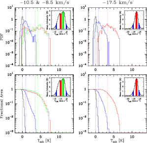
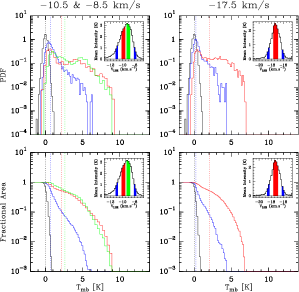
Figure 12: Left: Same as Fig. 5 but using the 30m data only. Right: Same as right but using the total field-of-view of the 30m data, i.e. $200^{\prime\prime}\times 200^{\prime\prime}$.

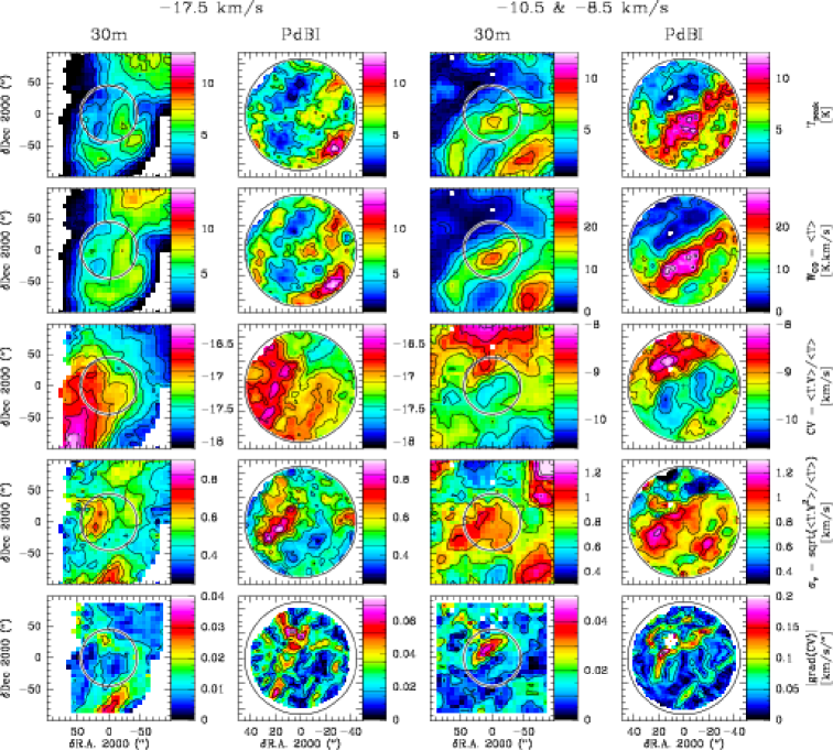
Figure 13: Moments of the components $-17.5\,\mathrm{km\,s^{-1}}$ and $-10.5$ and $-8.5\,\mathrm{km\,s^{-1}}$ together observed at two different resolution. From top to bottom: Peak temperature, Integrated area, Centroid velocity, 2nd order moment (proportional to the FWHM for a Gaussian line) and the modulus of the gradient of centroid velocity (for a flat rotation curve of the Galaxy, $-20\,\mathrm{km\,s^{-1}}$ corresponds to 2.5kpc in the direction of NRAO150 and at 2.5kpc, $0.1\,\mathrm{km\,s^{-1}}/^{\prime\prime}$ corresponds to $8\,\mathrm{km\,s^{-1}}\,\mbox{pc}^{-1}$).

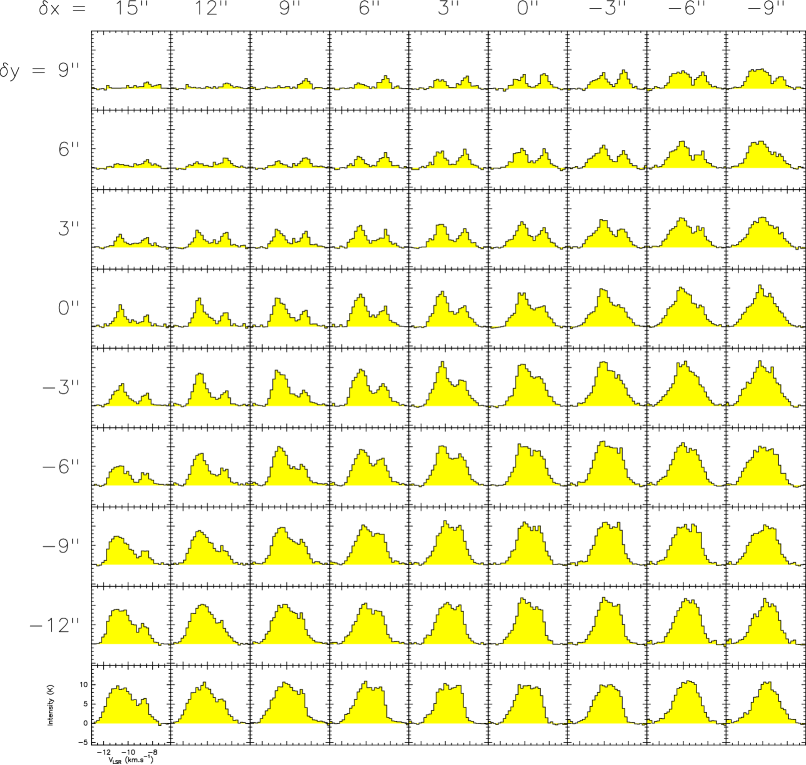
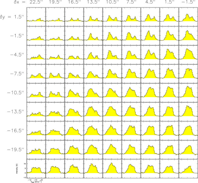
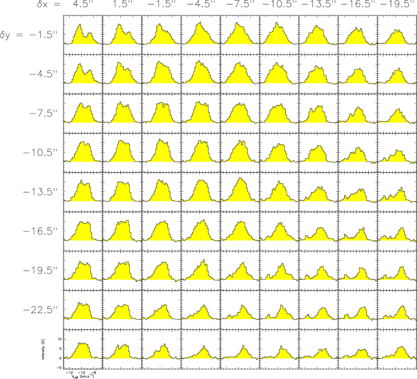
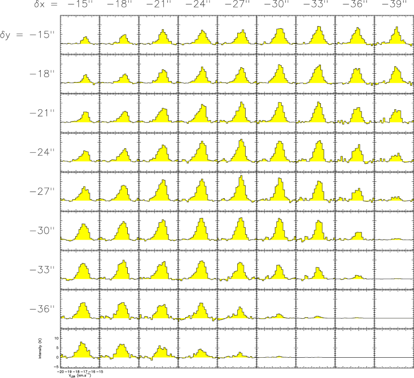
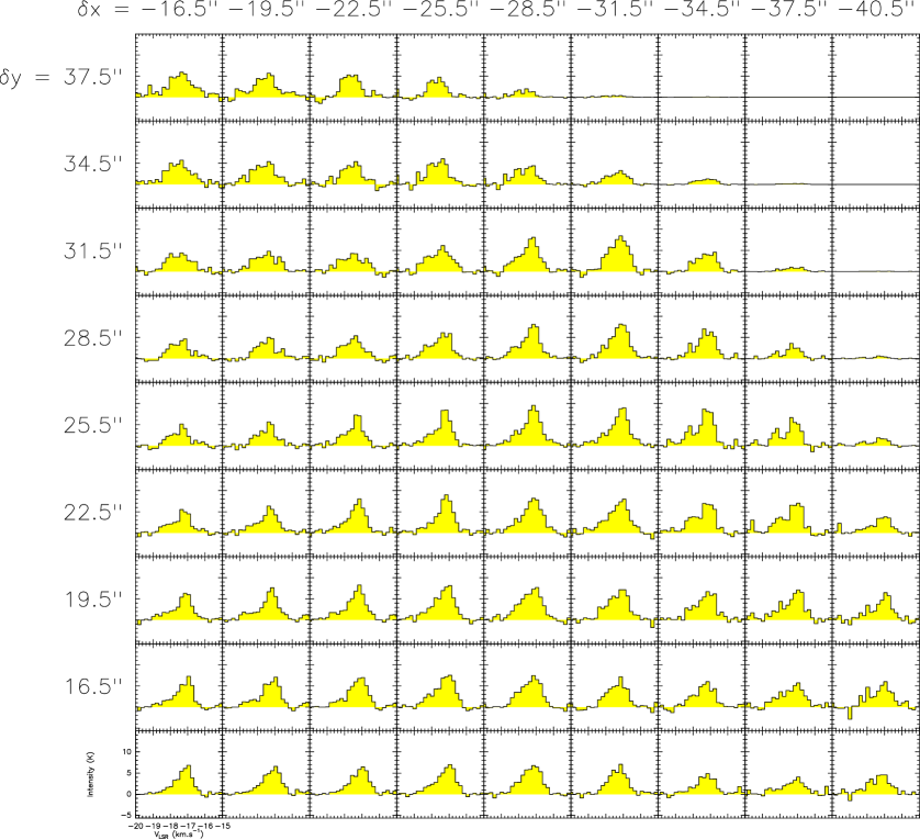
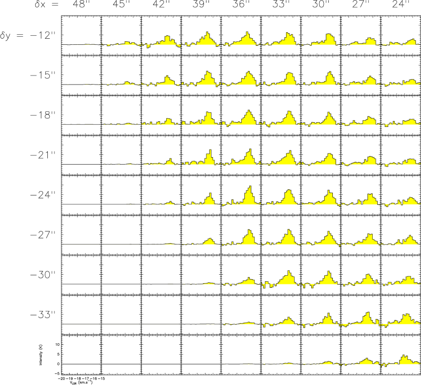
Figure 14: Maps of spectra around the profiles shown in Fig. 4 sorted by distance to NRAO150 from top to bottom. Left: The $-17.5\,\mathrm{km\,s^{-1}}$ feature shown around $(+3^{\prime\prime},-3^{\prime\prime})$, $(+10.5^{\prime\prime},-10.5^{\prime\prime})$ and $(-7.5^{\prime\prime},-13.5^{\prime\prime})$. Right: The $-10.5$ and $-8.5\,\mathrm{km\,s^{-1}}$ features shown around $(-27^{\prime\prime},-27^{\prime\prime})$, $-28.5^{\prime\prime},+25.5^{\prime\prime}$ and $(+36^{\prime\prime},-24^{\prime\prime})$.