Toward precise constraints on growth of massive black holes

Abstract

Growth of massive black holes (MBHs) in galactic centers comes mainly from gas accretion during their QSO/AGN phases. In this paper we apply an extended Sołtan argument, connecting the local MBH mass function with the time-integral of the QSO luminosity function, to the demography of MBHs and QSOs from recent optical and X-ray surveys, and obtain robust constraints on the luminosity evolution (or mass growth history) of individual QSOs (or MBHs). We find that the luminosity evolution probably involves two phases: an initial exponentially increasing phase set by the Eddington limit and a following phase in which the luminosity declines with time as a power law (with a slope of $\sim-1.2$—$-1.3$) set by a self-similar long-term evolution of disk accretion. Neither an evolution involving only the increasing phase with a single Eddington ratio nor an exponentially declining pattern in the second phase is likely. The period of a QSO radiating at a luminosity higher than 10% of its peak value is about 2–3$\times 10^{8}\rm yr$, during which the MBH obtains $\sim 80\%$ of its mass. The mass-to-energy conversion efficiency is $\simeq 0.16\pm 0.04^{+0.05}_{-0}$, with the latter error accounting for the maximum uncertainty due to Compton-thick AGNs. The expected Eddington ratios in QSOs from the constrained luminosity evolution cluster around a single value close to 0.5–1 for high-luminosity QSOs and extend to a wide range of lower values for low-luminosity ones. The Eddington ratios for high luminosity QSOs appear to conflict with those estimated from observations ($\sim 0.25$) by using some virial mass estimators for MBHs in QSOs unless the estimators systematically over-estimate MBH masses by a factor of 2–4. We also infer the fraction of optically obscured QSOs $\sim 60-80\%$. The constraints obtained above are not affected significantly by MBH mergers and multiple-times of nuclear activity (e.g., triggered by multiple times of galaxy wet major mergers) in the MBH growth history. We discuss further applications of the luminosity evolution of individual QSOs to obtaining the MBH mass function at high redshifts and the cosmic evolution of triggering rates of nuclear activity.

1. Introduction

Massive black holes (MBHs), probably remnants of QSOs (Lynden-Bell, 1969), have been detected in the nuclei of many nearby galaxies (Kormendy & Richstone, 1995; Magorrian et al., 1998; Richstone et al., 1998; Kormendy & Gebhardt, 2001; Ferrarese & Ford, 2005). How do these local MBHs form and evolve, and what is the most important mechanism shaping the mass distribution of MBHs? The current consensus is that the local MBHs obtained their mass mainly through accretion during phases of nuclear activity when they appeared as QSOs/AGNs, similar to the ones seen now in the distant universe (e.g., Yu & Tremaine, 2002; Yu & Lu, 2004a; Marconi et al., 2004; Shankar et al., 2004; Barger et al., 2005; Hopkins et al., 2006; Shankar et al., 2007). The evolution of mass accretion onto a MBH is equivalent to the luminosity evolution, given the mass-to-energy conversion efficiency, and is recorded in the luminosity function (LF) of QSOs. However, the QSO LF depends mainly on two functions: (1) ${\cal G}(z;M_{\bullet,0})$, the rate of nuclear activity triggered at different redshifts $z$ for MBHs with present-day mass $M_{\bullet,0}$; (2) ${\cal L}(\tau;M_{\bullet,0})$, the luminosity evolution history of a QSO, of which the remnant MBH has a present-day mass $M_{\bullet,0}$, as a function of the age of its nuclear activity $\tau$. One cannot derive these two functions only from the knowledge of the QSO LF without additional assumptions.

In an extended version of the Sołtan (1982) argument, the local MBH mass distribution function (BHMF) is related to QSOs found in the distant universe by the simple integral equation

$$\int^{\infty}_{0}\Psi_{L}(L,z)\left|\frac{dt}{dz}\right|dz = \int^{\infty}_{0}n_{M_{\bullet}}(M_{\bullet,0},t_{0})\times$$ (1)

$$\tau_{\rm lt}(M_{\bullet,0})P(L|M_{\bullet,0})dM_{\bullet,0},$$

where $t_{0}$ is the present cosmic time, $n_{M_{\bullet}}(M_{\bullet,0},t_{0})$ is the local BHMF, defined so that $n_{M_{\bullet}}(M_{\bullet,0},t_{0})dM_{\bullet,0}$ gives the number density of local MBHs with present-day mass in the range $M_{\bullet,0}\rightarrow M_{\bullet,0}+dM_{\bullet,0}$, $\Psi_{L}(L,z)$ is the QSO LF, defined so that $\Psi_{L}(L,z)dL$ gives the comoving number density of QSOs with nuclear luminosity in the range $L\rightarrow L+dL$ at redshift $z$,

$$\tau_{\rm lt}(M_{\bullet,0})=\int dL\sum_{k}\frac{1}{\left|\frac{d{\cal L}(\tau;M_{\bullet,0})}{d\tau}|_{\tau=\tau_{k}(L,M_{\bullet,0})}\right|}$$ (2)

is the time interval (or the QSO lifetime) in which that a MBH with present-day mass $M_{\bullet,0}$ appeared as a QSO, and $\tau_{k}(L,M_{\bullet,0})$ $(k=1,2,...)$ are the roots of the equation ${\cal L}(\tau;M_{\bullet,0})-L=0$ (see details of the derivation in Yu & Lu 2004a). Here ${\cal L}(\tau;M_{\bullet,0})$ represents the luminosity of a QSO and its associated MBH with present-day mass $M_{\bullet,0}$ at a time $\tau$ after the triggering of nuclear activity. The value of $\tau_{\rm lt}$ depends on the detailed definition of “active nuclei” or the lower threshold set to the nuclear luminosity. Finally,

$$P(L|M_{\bullet,0})=\frac{1}{\tau_{\rm lt}(M_{\bullet,0})}\sum_{k}\frac{1}{\left|\frac{d{\cal L}(\tau;M_{\bullet,0})}{d\tau}|_{\tau=\tau_{k}(L,M_{\bullet,0})}\right|}$$ (3)

is the probability distribution function of the nuclear (bolometric) luminosity $L$ over the growth history of the MBH. The right-hand-side of equation (1) gives the total time spent per unit $L$ at luminosity $L$ by the progenitors of all the local MBHs in a unit comoving volume, which should be the time integral of the QSO LF, i.e., the left-hand-side of the equation. Multiplying equation (1) by the BH mass accretion rate $(1-\epsilon)L/(\epsilon c^{2})=\dot{M}_{\bullet}$ (see eqs. 26 and 27 below), where $\epsilon$ is the mass-to-energy conversion efficiency and $c$ is the speed of light, and then integrating it over cosmic time $t$ reduces to the Sołtan (1982) argument (Yu & Lu, 2004a). Provided that two basic quantities, i.e., the local BHMF and the QSO LF, can be observationally determined with sufficient accuracy, the kernel $\tau_{\rm lt}(M_{\bullet,0})P(L|M_{\bullet,0})$, containing information on the luminosity evolution history of individual QSOs/MBHs, may be solved from the integral equation (1). Therefore, the extended Sołtan argument is expected to give robust but more detailed constraints on the growth of MBHs than the simple energetic argument due to Sołtan (1982).

As an alternative approach to the theoretical models based on the hierarchical co-evolution of MBHs and galaxies/galactic halos studied intensively in the literature (e.g., Efstathiou & Rees, 1988; Haehnelt & Rees, 1993; Haehnelt et al., 1998; Kauffmann & Haehnelt, 2000; Granato et al., 2001; Wyithe & Loeb, 2003; Volonteri et al., 2003; Croton et al., 2006; Bower et al., 2006; Malbon et al., 2007), in this paper we use the integral equation (1) to statistically constrain the growth history of individual MBHs or ${\cal L}$. The advantages of this approach are: (1) the accretion history of individual QSOs, ${\cal L}(\tau;M_{\bullet,0})$, is isolated from the triggering rate of nuclear activity, ${\cal G}(z;M_{\bullet,0})$, which is presumably associated with mergers of galaxies or instabilities of galactic disks; and (2) it is free of the many adjustable parameters introduced in the co-evolution models and probably also avoids uncertain assumptions on seed BHs. Note that these two functions, ${\cal G}(z;M_{\bullet,0})$ and ${\cal L}(\tau;M_{\bullet,0})$, are mixed in the differential continuity equation for BHMF evolution presented in Small & Blandford (1992, see also , , and ), which is widely used in studying the growth of MBHs (e.g., Marconi et al., 2004; Shankar et al., 2007). Using the luminosity evolution curves, i.e., ${\cal L}(\tau;M_{\bullet,0})$, obtained from numerical simulations of colliding galaxies, Hopkins et al. (2006) elaborated a unified model for the origin of QSOs and MBHs (see also their other papers listed therein). A possible concern with that approach is that simulations of colliding galaxies have a spatial resolution much larger than the scale of accretion disks around MBHs and therefore may not reflect the real luminosity evolution, as the disk accretion is probably self-regulated in the vicinity of MBHs rather than being directly determined by the material infall rate from a much larger scale or the Bondi-accretion rate (see discussions in § 4). (For another model of the possible light curve, see Ciotti & Ostriker 2007.)

Estimating the local BHMF can be done with recent advances in observations (e.g., Salucci et al., 1999; Aller & Richstone, 2002; Yu & Lu, 2004a; Marconi et al., 2004; Shankar et al., 2004; Lauer et al., 2007a; Tundo et al., 2007). First, MBHs are believed to exist in the nuclei of most, if not all, nearby galaxies (Kormendy & Richstone, 1995; Magorrian et al., 1998; Richstone et al., 1998; Kormendy & Gebhardt, 2001; Ferrarese & Ford, 2005). Second, it has been well established that tight correlations exist between the MBH mass and various galactic properties, such as mass, luminosity, stellar velocity-dispersion, light concentration and binding energy of the hot components of galaxies (here hot components mean either ellipticals or spiral bulges; Kormendy & Richstone, 1995; Magorrian et al., 1998; Ferrarese & Merritt, 2000; Gebhardt et al., 2000; Tremaine et al., 2002; Häring & Rix, 2004; Marconi & Hunt, 2004; Graham et al., 2001; Aller & Richstone, 2007). Third, the luminosity or velocity-dispersion functions of nearby galaxies have been well determined by large surveys such as the Sloan Digital Sky Survey (SDSS; Blanton et al., 2003; Bernardi et al., 2003; Sheth et al., 2003). Combining the correlation between the MBH mass and galaxy velocity dispersion (or luminosity) with the velocity-dispersion (or luminosity) distribution of nearby galaxies, we estimate the local BHMF in § 2.

In the past several years, the QSO LF has been determined over unprecedentedly large luminosity and redshift ranges both from optical surveys such as the Two Degree Field QSO Redshift Survey (2Qz) and SDSS, and from X-ray surveys by ASCA, Chandra and XMM-Newton. For example, the optical QSO LF has been obtained over the redshift range $0.4<z<2.1$ and the magnitude range $M_{\rm b_{J}}<-22.5$ using a sample of more than 15,000 QSOs from 2Qz (Croom et al., 2004); Richards et al. (2006a) estimated the QSO LF over a larger redshift range ($0.3<z<5$), but only for bright QSOs, using a homogeneous statistical sample of 15,343 QSOs drawn from SDSS Data Release 3; using the COMBO-17 data, Wolf et al. (2003) estimated the LF for faint QSOs over the range $1.2<z<4.8$; and Jiang et al. (2006) estimated the QSO LF over the range $0.5<z<3.6$ by using a deep survey of faint QSOs in the SDSS. Obscured (or type 2) QSOs may be missed in the optical surveys but can be detected in hard X-ray surveys. La Franca et al. (2005) use 508 AGNs to estimate the hard X-ray LF (HXLF; $2-10$ keV) over the range $0<z<2.5$ by combining data from XMM-Newton (Lockman hole) and the Chandra Deep Field (CDF). Barger et al. (2005) use a spectroscopically complete deep and wide-area Chandra survey to estimate the HXLF ($2-8$ keV) over the range $0<z<5$. Silverman et al. (2008) measure the HXLF ($2-8$ keV) up to $z\sim 5$ with fewer uncertainties by combining the observations from the CDF and the Chandra Multiwavelength Project. Combining all these observations, the time integrals of the QSO LF are estimated in § 3.

In § 4, we assume several models for the luminosity evolution history of individual QSOs, i.e., ${\cal L}(\tau;M_{\bullet,0})$, and then apply the models and the observational BHMF and QSO LF to equation (1) to give constraints on the growth of individual MBHs and the associated parameters, specifically, the efficiency (mainly determined by the spin of a MBH), the lifetime of nuclear activity, and the long-term evolution of disk accretion etc. We find that a reference model for the luminosity evolution history of individual QSOs, i.e., an initial rapid accretion phase with a rate close to the Eddington limit and then a following power-law declining phase set by the self-similar long-term evolution of disk accretion ($\dot{M_{\bullet}}\propto\tau^{-\gamma}$, and $\gamma\sim 1.2-1.3$), can satisfy the extended Sołtan argument (eq. 1) well. Using the reference model for ${\cal L}(M_{\bullet,0},\tau)$, we discuss the role of obscuration in the BH growth history in § 5 and find that obscuration is unlikely to be solely an evolutionary effect. The luminosity (or accretion-rate) evolution constrained by the extended Sołtan argument also implies a distribution of Eddington ratios (i.e., the accretion rate in units of the Eddington limit) in QSOs. In § 6, we particularly discuss its distribution expected from the models and compare them with observations. In § 7, by using toy models, we discuss the effects of BH mergers on our results, which are shown to be insignificant. In § 8, we discuss further implications of the luminosity evolution obtained from the extended Sołtan argument. Together with the QSO LF, ${\cal L}(\tau;M_{\bullet,0})$ can be used to further derive the BHMF at redshift $z$ and the triggering rate of nuclear activity ${\cal G}(z;M_{\bullet,0})$. Given ${\cal L}(\tau;M_{\bullet,0})$ and ${\cal G}(z;M_{\bullet,0})$, many statistical properties of QSOs can be inferred and comparison of them with observations may further deepen our understanding of the growth of MBHs. Conclusions are given in § 9.

In this paper we set the Hubble constant as $H_{0}=100h{\rm km~{}s^{-1}}{\rm\,Mpc}^{-1}$; and if not otherwise specified, the cosmological model used is $(\Omega_{m},\Omega_{\Lambda},h)=(0.3,0.7,0.7)$.

2. The mass function of MBHs at $z=0$

Studies of central MBHs in nearby galaxies have revealed strong correlations between the BH mass and the velocity dispersion (or luminosity, or other properties) of the hot stellar component of the host galaxy (e.g., Kormendy & Richstone, 1995; Magorrian et al., 1998; Ferrarese & Merritt, 2000; Gebhardt et al., 2000; Tremaine et al., 2002; Häring & Rix, 2004; Marconi & Hunt, 2004; Graham et al., 2001; Aller & Richstone, 2007; Hopkins et al., 2007b). We first present several latest fits of these correlations (i.e., the $M_{\bullet,0}-\sigma$ relation and the $M_{\bullet,0}-L_{\rm bulge}$ relation) and then present the observational velocity-dispersion (and luminosity) distribution of nearby galaxies. By combining them, we estimate the local BHMF in § 2.3.

2.1. The $M_{\bullet,0}-\sigma$ and $M_{\bullet,0}-L_{\rm bulge}$ relations

Lauer et al. (2007a) show that the logarithm of the BH mass at a given velocity dispersion $\sigma$ has a mean value given by

$$\langle\log M_{\bullet,0}|\log\sigma\rangle = (8.29\pm 0.07)+(4.13\pm 0.32)\times$$ (4)

$$\log\left(\frac{\sigma}{200{\rm km~{}s^{-1}}}\right),$$

which is fitted in the $(\log M_{\bullet,0},\log\sigma)$ space. The mean value at a given $V$-band absolute magnitude $M_{V}$ is given in the same paper as

$$\langle\log M_{\bullet,0}|M_{V}\rangle=(8.67\pm 0.09)-\frac{(1.32\pm 0.14)}{2.5}(M_{V}+22).$$ (5)

The intrinsic scatters around the relations above are not reported in Lauer et al. (2007a). (Hereafter the intrinsic scatters in $\log M_{\bullet,0}$ are noted as $\Delta_{M_{\bullet,0}-\sigma}$ and $\Delta_{M_{\bullet,0}-L_{\rm bulge}}$ for the $M_{\bullet,0}-\sigma$ relation and $M_{\bullet,0}-L_{\rm bulge}$ relation, respectively.) Based on the same sample, Tremaine et al. (2002) estimate that the intrinsic scatter in $\log M_{\bullet,0}$ for the $M_{\bullet,0}-\sigma$ relation, i.e., $\Delta_{M_{\bullet,0}-\sigma}$, should be not larger than $0.25-0.3$ dex. The latest fit of the $M_{\bullet}-\sigma$ relation by Hu (2008), which is consistent with that given by Lauer et al. (2007a) on the zero point and the slope, also gives an upper limit to the intrinsic scatter $\sim 0.25$ dex. Note also the zero point in equation (4) is larger than that obtained by Tremaine et al. (2002) by $0.10$ dex, but roughly consistent with statistical errors.

The estimates of the $M_{\bullet,0}-\sigma$ and $M_{\bullet,0}-L_{\rm bulge}$ relations in Bernardi et al. (2007) are given by:

$$\langle\log M_{\bullet,0}|\log\sigma\rangle = (8.21\pm 0.05)+(3.83\pm 0.10)\times$$ (6)

$$\log\left(\frac{\sigma}{200{\rm km~{}s^{-1}}}\right),$$

and

$$\langle\log M_{\bullet,0}|M_{r}\rangle=(8.57\pm 0.10)-\frac{(1.30\pm 0.10)}{2.5}(M_{r}+22),$$ (7)

with intrinsic scatters not larger than $0.22\pm 0.05$ dex and $0.33\pm 0.08$ dex, respectively. Another set of fits to equation (7) by the same authors (Tundo et al., 2007) finds a slope $1.30\pm 0.15$ and the zero point is $8.68\pm 0.10$, consistent with statistical errors. If we convert $M_{r}$ to $M_{V}$ with $M_{r}=M_{V}-0.37$ adopted for early-type galaxies (Fukugita et al., 1996), we find the zero point in equation (7) is larger than that in equation (5) by $0.09$ dex.

The typical difference in the zero point among different sets of fits to the $M_{\bullet,0}-\sigma$ (or $M_{\bullet,0}-L_{\rm bulge}$) relation is $\lesssim 0.10$ dex, which is roughly consistent with the statistical errors in the zero point estimation. The difference in the slope among different sets of fits to the $M_{\bullet,0}-\sigma$ relation is quite large compared to the statistical errors in the fits, for example, it is $4.13\pm 0.32$ in Lauer et al. (2007a), $3.83\pm 0.10$ in Bernardi et al. (2007), and $4.86\pm 0.43$ in Ferrarese & Ford (2005) (for details of the difference in the slope see discussions in Tremaine et al. 2002). Note that Aller & Richstone (2007) investigate an alternative relation to the $M_{\bullet,0}-\sigma$ relation; and they find that the relation between the MBH mass and the bulge gravitational binding energy is as good as the $M_{\bullet,0}-\sigma$ relation in predicting MBH mass but with a slope much more stable regarding of changes in the fitting algorithm. A detailed study by Novak et al. (2006) demonstrates that the upper limit to the intrinsic scatter is $\sim 0.2-0.3$ dex in the $M_{\bullet,0}-\sigma$ relation and is $\sim 0.3-0.4$ dex in the $M_{\bullet,0}-L_{\rm bulge}$ relation for currently available samples. Below we adopt $\Delta_{M_{\bullet,0}-\sigma}\sim 0.3$ dex relation and $\Delta_{M_{\bullet,0}-L_{\rm bulge}}\sim 0.4$ dex if not otherwise specified.

Among the subtle differences in zero points, slopes and intrinsic scatters of those relations estimated by different groups, the intrinsic scatter would be the most significant one for the purpose of studying MBH growth, because it may affect the estimates of the abundance of MBHs at the high-mass end ($\gtrsim 10^{9}M_{\odot}$) by orders of magnitude (as shown in Fig. 1 below; see also discussions in Yu & Lu 2004a; Marconi et al. 2004; Lauer et al. 2007a; Tundo et al. 2007), and this abundance is crucial for our understanding of the growth of the most massive BHs in bright QSOs.

2.2. The velocity-dispersion distribution function and the luminosity function of nearby galaxies

We define $n_{\sigma}(\sigma,t)$ as the comoving velocity-dispersion function of the hot stellar components of local galaxies so that $n_{\sigma}(\sigma,t_{0}){\rm d}\sigma$ represents the number density of local galaxies in the range $\sigma\rightarrow\sigma+{\rm d}\sigma$. The velocity-dispersion distribution $n_{\sigma}(\sigma,t_{0})$ includes the contribution from both early-type galaxies $n^{\rm e}_{\sigma}(\sigma,t_{0})$ and bulges of late-type galaxies $n^{\rm l}_{\sigma}(\sigma,t_{0})$, that is,

$$n_{\sigma}(\sigma,t_{0})=n^{\rm e}_{\sigma}(\sigma,t_{0})+n^{\rm l}_{\sigma}(\sigma,t_{0}).$$ (8)

• The velocity-dispersion distribution in early-type galaxies has been estimated by recent studies of a sample of early-type galaxies at $z<0.3$ obtained by the SDSS (see eq. 4 in Sheth et al. 2003, and Bernardi et al. 2003):

  $$n^{\rm e}_{\sigma}(\sigma,t_{0})=\phi_{*}\left(\frac{\sigma}{\sigma_{*}}\right)^{\alpha}\frac{\exp\left[-(\sigma/\sigma_{*})^{\beta}\right]}{\Gamma(\alpha/\beta)}\frac{\beta}{\sigma},$$ (9)

  where the best-fit values of $(\phi_{*},\sigma_{*},\alpha,\beta)$ are $(0.0020\pm 0.0001,88.8\pm 17.7,6.5\pm 1.0,1.93\pm 0.22)$, $\phi_{*}$ is the comoving number density of local early-type galaxies in units of $h^{3}_{0.7}{\rm\,Mpc}^{-3}$, and $\sigma_{*}$ is in units of ${\rm km~{}s^{-1}}$. The brightest cluster galaxies (BCGs) are probably under-represented in the above sample (Lauer et al., 2007a). We correct this by adding the number density of BCGs to equation (9), where the number density of BCGs with $\sigma>350{\rm km~{}s^{-1}}$ is estimated from the sample of Bernardi et al. (2006) as done in Lauer et al. (2007a). If the scatter in the $M_{\bullet,0}-\sigma$ (or $M_{\bullet,0}-L_{\rm bulge}$) relation is not significantly smaller than $0.3$ dex (or $0.4$ dex), this correction is not significant because most of high-mass MBHs (larger than a few $10^{9}M_{\odot}$) actually come from ‘modest’ galaxies with unusually large MBHs for their velocity dispersions or luminosities (see the dependence of the BHMF on different values of the scatter in Fig. 1; see also Lauer et al. 2007b).

• The velocity-dispersion distribution in late-type galaxies $n_{\sigma}^{\rm l}(\sigma,t_{0})$ may be estimated in the following ways. (i) Following Sheth et al. (2003), the LF of the late-type galaxies can be obtained by subtracting the LF of the early-type galaxies (Bernardi et al., 2003) from the total LF of all galaxies (Blanton et al., 2003). (ii) Following Sheth et al. (2003), the distribution of the circular velocity $v_{\rm c}$ in late-type galaxies may be obtained by using the LF of the late-type galaxies obtained above and the following Tully-Fisher relation (Giovanelli et al., 1997)

  $$\log\left(\frac{2v_{\rm c}}{{\rm km~{}s^{-1}}}\right)=1.00-(M_{I}-5\log h_{0.7})/7.95,$$ (10)

  where $M_{I}$ is the absolute magnitude of the galaxies in the $I$ band, with accounting for the intrinsic scatter around relation (10) and the inclination effects of galaxies (see details in Sheth et al. 2003). (iii) The velocity-dispersion function of late-type galaxies can be obtained by using the circular-velocity distribution of the late-type galaxies obtained above and the following relation between the circular velocity and the velocity dispersion of the bulge component (see eq. 3 in Baes et al. 2003, and also Ferrarese 2002):

  $$\log\left(\frac{v_{\rm c}}{200{\rm km~{}s^{-1}}}\right) = (0.96\pm 0.11)\log\left(\frac{\sigma}{200{\rm km~{}s^{-1}}}\right)$$ (11)

  $$+(0.21\pm 0.023).$$

  The intrinsic scatter of relation (11) is small ($<0.15{\rm\,dex}$, see Fig. 1 in Baes et al. 2003) and will be ignored in our calculations. We could also simply use $\sigma=v_{\rm c}/\sqrt{3}$ (e.g., see problem 4.35 in Binney & Tremaine 2008) to estimate $\sigma$, which only induces a slight difference in estimating the BHMF. Relation (11) may not hold for $\sigma<80{\rm km~{}s^{-1}}$, which corresponds to $M_{\bullet,0}\lesssim 4\times 10^{6}M_{\odot}$ according to the $M_{\bullet,0}-\sigma$ relation above (eqs. 4 and 6), but this is beyond the main range which we focus on in § 4. Note that the local BHMF for mass $M_{\bullet,0}\gtrsim 4\times 10^{7}M_{\odot}$ is dominated by the early-type galaxies (see also Fig. 1 in Yu & Lu 2004a).

The LF of galaxies is conventionally described by the Schechter (1976) function:

$$\Phi(M) = 0.4\ln(10){\phi}_{\ast}10^{-0.4(M-M_{*})(\alpha+1)}\times$$ (12)

$$\exp[-10^{-0.4(M-M_{*})}],$$

where $\Phi(M)dM$ gives the comoving number density of galaxies with absolute magnitude in the range $M\rightarrow M+dM$. Based on observations by the SDSS (Blanton et al., 2003), the best fit parameters [${\phi}_{*}/(10^{-2}h^{3}_{0.7}{\rm\,Mpc}^{-3})$, $M_{*}-5\log h_{0.7}$, $\alpha$] of the LFs are ($6.36\pm 0.23$, $-18.62\pm 0.02$,$-0.89\pm 0.03$) in the $g$ band and ($4.34\pm 0.12$,$-19.67\pm 0.01$,$-1.05\pm 0.01$) in the $r$ band, respectively. Here $M$ is the absolute magnitude of a galaxy (not just of its hot stellar component). We can crudely estimate the luminosity of the hot stellar component of a galaxy, for which the relations in equations (5) and (7) are applied, from the total luminosity of the galaxy $L_{\rm gal}$ by setting $L_{\rm bulge}=(L_{\rm gal}/L_{*})/(1+L_{\rm gal}/L_{*})L_{\rm gal}$ (e.g., Tundo et al., 2007). With this modification, the BHMF can be estimated using either the $M_{\bullet,0}-M_{V}$ relation (eq. 5) or the $M_{\bullet,0}-M_{r}$ relation (eq. 7) and the galaxy LF in the $g$ band (with a color correction of $g=M_{V}+0.41$; Fukugita et al. 1995) or the $r$ band.

2.3. $n_{M_{\bullet}}(M_{\bullet,0},t_{0})$

We show in Figure 1 the BHMF obtained by combining the $M_{\bullet,0}-\sigma$ (or $M_{\bullet,0}-L_{\rm bulge}$) relation with the velocity-dispersion (or luminosity) distribution function of local galaxies (e.g., see eq. 44 in Yu & Lu 2004a). Our calculations show that the uncertainties in the intrinsic scatter of the $M_{\bullet,0}-\sigma$ (or $M_{\bullet,0}-L_{\rm bulge}$) relation may affect estimates of the BHMF significantly at the high-mass end (see Fig. 1). To illustrate this effect, we assume that the intrinsic scatters in the $M_{\bullet,0}-\sigma$ (or $M_{\bullet,0}-L_{\rm bulge}$) relation by Lauer et al. (2007a) (eqs. 4 and 5) and by Bernardi et al. (2007) (eqs. 6 and 7) are 0, 0.2 and 0.3 dex (or 0, 0.3 and 0.4 dex), respectively. With the intrinsic scatter of the $M_{\bullet,0}-\sigma$ (or $M_{\bullet,0}-L_{\rm bulge}$) relation $\sim 0.3$ dex (or $\sim 0.4$ dex), the estimated abundance of MBHs at the high-mass end ($\gtrsim 10^{9}M_{\odot}$) is larger than that estimated from a zero intrinsic scatter by orders of magnitude (see the upper panels of Fig. 1). The difference in the slope and the zero point among different sets of fits to the $M_{\bullet,0}-\sigma$ (or $M_{\bullet,0}-L_{\rm bulge}$) relation may also affect the estimates of the abundance of MBHs at the high-mass end, but its effects are substantially less significant compared to that of the intrinsic scatter (see Fig. 1 and also Yu & Lu 2004a).

As shown in the bottom left panel of Figure 1, the abundance of MBHs estimated from the $M_{\bullet,0}-L_{\rm bulge}$ relation is larger than that from the $M_{\bullet,0}-\sigma$ relation roughly by a factor $\sim 2$ if both relations are adopted from Lauer et al. (2007a) (see also discussions in Lauer et al. 2007a and Tundo et al. 2007), but the shapes are similar. One possible reason for this discrepancy in abundance is that the local MBH sample used to derive the $M_{\bullet,0}-L_{\rm bulge}$ relation is biased relative to the SDSS galaxy sample as discussed in Yu & Tremaine (2002) and Bernardi et al. (2007). (The other possibility is systematic differences in measurements of luminosity or velocity dispersion between other surveys and the SDSS.) If we correct this ‘bias’ with the recipe introduced in Tundo et al. (2007), then the BHMF estimated from the $M_{\bullet,0}-L_{\rm bulge}$ relation is almost the same as that estimated from the $M_{\bullet,0}-\sigma$ relation at the high-mass end ($M_{\bullet,0}\gtrsim$ a few $10^{8}M_{\odot}$), as shown in the bottom right panel of Figure 1. The remaining discrepancy at the low-mass end is possibly due to uncertainties in the estimation of the bulge luminosity from the total luminosity for late-type galaxies. For example, recent studies by Laurikainen et al. (2005) and Graham & Worley (2008) have shown that the bulge-to-total luminosity ratio (B/T ratio) is around 0.24 for S0 galaxies, which is substantially smaller than the previous estimates ($\sim 0.6$; e.g., Fukugita et al. 1998). According to these new estimates, the B/T ratio adopted in Tundo et al. (2007) may be an overestimate at least for S0 galaxies, and thus the BHMF at the low-mass end $\lesssim 10^{8}M_{\odot}$ is probably substantially overestimated. (The B/T ratio adopted in other estimates of the BHMF may be also overestimated; e.g., Marconi et al. 2004.) It is anticipated that the BHMF at the low-mass end estimated by using the $M_{\bullet,0}-L_{\rm bulge}$ relation will be closer to that estimated by using the $M_{\bullet,0}-\sigma$ relation if adopting a more realistic B/T ratio for spiral galaxies. In § 4, we adopt the BHMF obtained from the $M_{\bullet,0}-\sigma$ relation given by Lauer et al. (2007a) with an intrinsic scatter of $0.3$ dex as the reference BHMF, if not otherwise specified.

In addition to the uncertainty on the local BHMF due to the intrinsic scatter in the $M_{\bullet,0}-\sigma$ (or $M_{\bullet,0}-L_{\rm bulge}$) relation, the local BHMF suffers other uncertainties, in particular, the uncertainties in estimating the $M_{\bullet,0}-\sigma$ (or $M_{\bullet,0}-L_{\rm bulge}$) relation [e.g., due to (1) limited mass range and small samples; (2) being restricted to ellipticals, and little is known about late-type galaxies; (3) determining $M_{\bullet,0}$ is difficult and may be underestimated, especially for BCGs] and the uncertainties in estimating the velocity-dispersion (or bulge luminosity) distribution in late-type galaxies.

The total mass density of local MBHs can be estimated from the BHMF. The differences in the zero point, the slope and the intrinsic scatter among the relations estimated by different groups could cause at most a 20-30% difference in the total mass density of local MBHs (as shown in § 2.1). For example, adopting the $M_{\bullet,0}-\sigma$ relation given by Lauer et al. (2007a) yields a total mass density of MBHs $\simeq 3.8^{+0.7}_{-0.6}\times 10^{5}h_{0.7}^{2}M_{\odot}{\rm Mpc}^{-3}$, which is larger than that obtained by Yu & Tremaine (2002) by a factor of $\sim 1.3$ mainly due to the larger zero point of the $M_{\bullet,0}-\sigma$ relation in Lauer et al. (2007a) adopted here. We show in Table LABEL:tab:1 a few estimates of the total mass density of local MBHs obtained from the $M_{\bullet,0}-\sigma$ (or $M_{\bullet,0}-L_{\rm bulge}$) relation given by different authors. The errors are obtained by accounting for the uncertainties in the $M_{\bullet,0}-\sigma$ (or $M_{\bullet,0}-L_{\rm bulge}$) relation and the galaxy velocity-dispersion (or the luminosity) distribution function. (For other estimates of the total mass density of local MBHs, see Tab. 3 in Graham 2007.) The total mass density obtained from the $M_{\bullet,0}-L_{\rm bulge}$ relation is about a factor of $\sim 2$ larger than that obtained from the $M_{\bullet,0}-\sigma$ relation, which is consistent with that in Yu & Tremaine (2002) (see also discussions for the reasons of this discrepancy in Tundo et al. 2007). If we use the recipe introduced by Tundo et al. (2007) to correct the possible bias in MBH masses estimated from the $M_{\bullet,0}-L_{\rm bulge}$ relation, the corrected total mass densities are still larger than that obtained from the $M_{\bullet,0}-\sigma$ relation but now appears to be consistent within statistical errors (see Tab. LABEL:tab:1). Furthermore, considering that the B/T ratio for spiral galaxies adopted in the estimates of total BH mass density using the $M_{\bullet,0}-L_{\rm bulge}$ relation is probably an overestimate, the total BH mass density from the $M_{\bullet,0}-L_{\rm bulge}$ and the galaxy LF may be actually not much different from that estimated from the $M_{\bullet,0}-\sigma$ relation and the galaxy velocity dispersion distribution function.

Table 1The total mass density of massive black holes

Method	Reference	Note	$\frac{\rho_{\bullet,0}}{10^{5}M_{\odot}}$
$M_{\bullet,0}-\sigma$	Lauer07a	……	$3.8^{+0.7}_{-0.6}$
$M_{\bullet,0}-\sigma$	Bernardi07	……	$3.3^{+0.5}_{-0.4}$
$M_{\bullet,0}-\sigma$	FF05	……	$3.6^{+0.7}_{-0.6}$
$M_{\bullet,0}-L_{\rm bulge}$	Lauer07a	……	$7.6^{+2.0}_{-1.7}$
$M_{\bullet,0}-L_{\rm bulge}$	Bernardi07	……	$8.5^{+2.4}_{-2.0}$
$M_{\bullet,0}-L_{\rm bulge}$	Lauer07a	Bias corrected	$4.9^{+1.3}_{-1.0}$
$M_{\bullet,0}-L_{\rm bulge}$	Bernardi07	Bias corrected	$4.3^{+1.2}_{-1.0}$

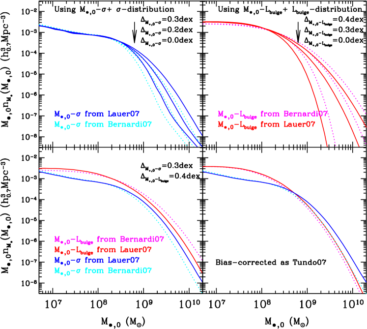
Figure 1.— The local BHMF obtained from the velocity-dispersion/luminosity distribution function of nearby galaxies and the MBH mass versus velocity-dispersion/luminosity relation (see details in § 2). Upper left panel: the solid lines represent $M_{\bullet,0}n_{M_{\bullet}}(M_{\bullet,0},t_{0})$ obtained from the $M_{\bullet,0}-\sigma$ relation given in Lauer et al. (2007a, here Lauer07), with assumed intrinsic scatters $\Delta_{M_{\bullet}-\sigma}=0.3$, $0.2$, and $0$ dex from top to bottom, respectively; while the dotted lines represent the $M_{\bullet,0}n_{M_{\bullet}}(M_{\bullet,0},t_{0})$ obtained from the $M_{\bullet,0}-\sigma$ relation given in Bernardi et al. (2007, here Bernardi07) with the same assumed intrinsic scatters. The velocity-dispersion distribution is obtained from equation (8). Upper right panel: BHMF estimated from the galaxy luminosity function and the $M_{\bullet,0}-L_{\rm bulge}$ relation with assumed intrinsic scatter $\Delta_{M_{\bullet}-L_{\rm bulge}}=0.4$, $0.3$ and $0$ dex from top to bottom, respectively. The solid lines represent the BHMF obtained from the $M_{\bullet,0}-L_{\rm bulge}$ relation given in Lauer07, while dotted lines for the relation given in Bernardi07. The bulge luminosity of a galaxy is used here by modifying the galaxy luminosity function to the bulge luminosity function as shown in § 2.2. Bottom left panel: comparison of the BHMF obtained from the $M_{\bullet,0}-\sigma$ relation and that obtained from the $M_{\bullet,0}-L_{\rm bulge}$ relation for the relations estimated either in Lauer07a or in Bernardi07. The intrinsic scatter for the $M_{\bullet,0}-\sigma$ (or $M_{\bullet,0}-L_{\rm bulge}$) relation is assumed to be $\Delta_{M_{\bullet}-\sigma}=0.3$ dex (or $\Delta_{M_{\bullet}-L_{\rm bulge}}=0.4$ dex), which is taken as the most probable number in this paper. Bottom right panel: similar to the bottom left panel but with corrections for bias as suggested by Tundo et al. (2007, here Tundo07).

3. The QSO/AGN LF in the optical and hard X-ray bands

3.1. The optical QSO LF

The optical QSO LF was first estimated by Schmidt (1968) and Schmidt & Green (1983), and it has been investigated extensively since then. The shape and evolution of the QSO LF has been well, though not perfectly, constrained due to recent surveys with unprecedentedly large redshift and luminosity spans (e.g., Boyle et al., 2000; Wolf et al., 2003; Croom et al., 2004; Richards et al., 2005, 2006a; Jiang et al., 2006; Fontanot et al., 2007; Siana et al., 2007). Using a sample of more than 15,000 QSOs at redshift $z<2.5$ from 2Qz and 6Qz, Croom et al. (2004) obtained the binned QSO LF $\Psi_{M}(M_{{\rm b_{J}},i},z_{j})$ over the range $0.4<z<2.1$ and the magnitude range $M_{\rm b_{J}}<-22.5$, where $M_{{\rm b_{J}},i}$ is the $i$th bin of the absolute magnitude and $z_{j}$ is the $j$th bin of the redshift. For some high-redshift bins, the binned QSO LF at low luminosity is not available because of the flux limit of the surveys. The time integral of the QSO LF can be estimated through direct summation by multiplying the binned QSO LF by the cosmic time duration as

$${\cal T}^{\prime}_{M_{\rm b_{J},QSO}}=\sum_{j}\Psi_{M}(M_{{\rm b_{J}},i},z_{j})\Delta t(z_{j}),$$ (13)

where $\Delta t(z_{j})$ is the cosmic time interval corresponding to the redshift bin $z_{j}$, $\Psi$ is assumed to be 0 outside observational bins, and the prime ^′ indicates the value obtained by summation over bins—in contrast the variable ${\cal T}$ without prime (see eq. 15) represents the time integral of a continuous fit to the QSO LF. These summations only give lower limits to the time integral of the QSO LF because the binned QSO LF, especially in the low-luminosity bins, does not extend to high enough redshift to include all QSOs. Richards et al. (2006a) obtained the binned QSO LF over a larger redshift range ($0.3<z<5$) using a homogeneous statistical sample of 15,343 QSOs drawn from SDSS Data Release 3. Unfortunately, the SDSS survey is shallow so the binned QSO LF can only be determined at the bright end. As a complement to the above estimates, the QSO LF for faint QSOs over the range $1.2<z<4.8$ was estimated by Wolf et al. (2003) using the COMBO-17 data; by Jiang et al. (2006) over the range $0.5<z<3.6$ using a deep survey of faint QSOs in the SDSS; by Fontanot et al. (2007) in the redshift range $3.5<z<5.2$ by combining the data from the Great Observatories Origins Deep Survey (GOODS) and the SDSS; and by Siana et al. (2007) at the redshift range $2.83<z<3.44$ using the data from the Spitzer Wide-area Infrared Extragalactic (SWIRE) Legacy Survey. In Figure 2, the direct summations (eq. 13) are shown for the binned QSO LF from Croom et al. (2004, blue triangles), Wolf et al. (2003, magenta circles) and Richards et al. (2006a, green squares), respectively (the $M_{i}$ magnitude in Richards et al. 2006a and $M_{145}$ magnitude in Wolf et al. 2003 are all converted to $M_{B}$ magnitude by $M_{\rm B}\simeq M_{i}(z=2)+0.80$ and $M_{\rm B}=M_{145}+1.75$, see Richards et al. 2006a and Wolf et al. 2003). At the high-luminosity end, the estimate from Croom et al. (2004) is substantially smaller than that from Richards et al. (2006a) which emphasizes the significance of the contribution from high-redshift QSOs. At the low-luminosity end, the estimates from Richards et al. (2006a) are smaller than those from others because the Richards et al. (2006a) sample is shallower and the majority of faint QSOs are not included.

We combine these binned QSO LFs obtained by different surveys over different redshift and luminosity ranges (Croom et al., 2004; Wolf et al., 2003; Richards et al., 2006a; Jiang et al., 2006; Fontanot et al., 2007; Siana et al., 2007), to cover luminosity and redshift ranges as large as possible. The basic rule is that the binned QSO LF from the largest sample are adopted at each redshift bin with data available and interpolations of the data points over magnitudes at a given redshift are used. The red points in Figure 3 are the estimated ${\cal T}^{\prime}_{M_{\rm B,QSO}}$ with mean magnitude corresponding to that in Croom et al. (2004). At bright magnitudes, most of the points cover the range $0.4<z\lesssim 5$ but the two points with faintest magnitudes only cover the range $0.4<z<1.0$. In addition, the five green squares represent the brightest QSOs obtained from Richards et al. (2006a) only and are consistent with the trend of the red points.

The optical QSO LF is frequently fitted with a double power law:

$$\Psi_{M}(M,z)=\frac{\Psi_{M}^{*}}{10^{0.4(\beta_{1}+1)[M-M^{*}(z)]}+10^{0.4(\beta_{2}+1)[M-M^{*}(z)]}},$$ (14)

where $\Psi_{M}(M,z)dM$ is the comoving number density of QSOs with absolute magnitude in the range [$M,M+dM$] at redshift $z$. That is, the evolution of the QSO LF can be characterized by three functions of redshift: the slopes at both the high-luminosity ($\beta_{1}$) and the low-luminosity ends ($\beta_{2}$) and the break luminosity (corresponding to $M^{*}$). Boyle et al. (2000), Croom et al. (2004), Richards et al. (2005), and Jiang et al. (2006) all use this functional form to fit their data sets from 2dF and SDSS, except that Jiang et al. (2006) introduced additional density evolution to the QSO LF at high redshift ($z>2.0$). Adopting their best-fit models, the time integral of the QSO LF,

$${\cal T}_{M_{\rm QSO}}=\int\Psi_{M}(M,z)\frac{dt}{dz}dz,$$ (15)

is obtained by integrating the QSO LFs over the range $0<z<8$. This function is shown in Figures 2 and 3. There are some differences in the model parameters among the best-fit models for different samples. For example, Croom et al. (2004) obtained a slope of $\beta_{2}\sim 1.09$ at the faint end (blue line), but Richards et al. (2005) obtained a steeper slope ($\beta_{2}\sim 1.45$; green line) using a sample from the 2dF-SDSS LRG and QSO survey (2SLAQ) with a flux limit of one magnitude fainter, which is roughly consistent with that obtained by Boyle et al. (2000) ($\beta_{2}\sim 1.58$; red line). Jiang et al. (2006) also obtained a shallower slope ($\beta_{2}\sim 1.25$; cyan line) with a deep survey in the SDSS, which is similar to that ($\beta_{2}=1.24$) found by Hunt et al. (2004) at redshift $z\sim 3$. At high redshift ($z\gtrsim 3$), the estimate of the faint-end slope by Fontanot et al. (2007) is consistent with $\beta_{2}=1.45$ but may have a high probability to be as steep as $\beta_{2}=1.71$, and Siana et al. (2007) obtained $\beta_{2}=1.42$, which is not inconsistent with values measured at lower redshift (e.g., Richards et al., 2005; Boyle et al., 2000). The differences in $\beta_{2}$ are the primary reason for the differences in ${\cal T}_{M_{\rm B,QSO}}$ at the faint end (see Figs. 2 and 3). (Below we choose $\beta_{2}\sim 1.45$ as the best estimate of the faint end of the QSO LF in § 5.) At the high luminosity end, the direct summations from the combination of the binned QSO LFs (according to eq. 13), which should be a lower limit to the time integrals, are quite consistent with the integration obtained from extrapolations of the best-fit analytic models, which may suggest that the estimates of ${\cal T}_{M_{\rm B,QSO}}$, at least at the high-luminosity end, are quite secure.

3.2. X-ray AGN LF

The advantage of counting QSOs/AGNs in X-rays is that relatively low-luminosity AGNs and obscured (type-2) AGNs, which may be missed in optical surveys, can be unambiguously detected in deep X-ray surveys even at large redshift. Although the number of QSOs/AGNs observed in X-rays ($\lesssim 1000$) is still substantially smaller than that observed in the optical band ($>10^{4}$), the X-ray AGN (XAGN) LF can be estimated with considerable accuracy (e.g., Ueda et al., 2003; La Franca et al., 2005; Hasinger et al., 2005; Barger et al., 2005; Silverman et al., 2008). Ueda et al. (2003) estimated the hard X-ray ($2-10$ keV) LF (HXLF), which is assumed to represent the total X-ray LF of unobscured plus Compton-thin AGNs, from a complete sample with $\sim 257$ sources observed by ASCA (but most of their sources have redshift $z<3$). La Franca et al. (2005) estimated the HXLF using a combined sample with $508$ sources with redshift $z\lesssim 2.5$. With the data from Chandra deep surveys, Barger et al. (2005) extended the estimate of the HXLF ($2-8$ keV) to higher redshift ($3\lesssim z\leq 5$) but with large uncertainties at this redshift range. Combining the published data from deep surveys by Chandra (i.e., CDF-North, CDF-South) and XMM-Newton (Lockman Hole) and rare luminous sources from the Chandra Multiwavelength Project, Silverman et al. (2008) estimated the HXLF ($2-8$ keV) at redshift $3\lesssim z\lesssim 5$ with much smaller uncertainties. The soft X-ray ($0.5-2$ keV) LF recently computed by Hasinger et al. (2005) is assumed to represent the unobscured type-1 AGNs. Gilli et al. (2007) demonstrated that the soft X-ray LF obtained by Hasinger et al. (2005) is actually consistent with the HXLF obtained by Ueda et al. (2003) and La Franca et al. (2005) by assuming a distribution of absorption column densities. However, the bolometric correction (BC) for the soft X-ray band is much more uncertain than that in the hard X-ray band, so we shall not consider the soft X-ray LF further in this paper. The shape and evolution of the X-ray LF in both hard X-ray and soft X-ray bands can be described by the “luminosity-dependent density evolution” model (e.g., Ueda et al., 2003; La Franca et al., 2005; Silverman et al., 2008; Miyaji et al., 2000; Hasinger et al., 2005):

$$\Psi_{\log L}(\log L_{X},z)=\frac{d\psi(<L_{X},z)}{d\log L_{X}}=\frac{d\psi(<L_{X},z=0)}{d\log L_{X}}e(z),$$ (16)

where $\Psi_{\log L}(\log L_{X},z)d\log L_{X}$ is the comoving number density of QSOs with logarithm X-ray luminosity in the range [$\log L_{X}$, $\log L_{X}+d\log L_{X}$],

$$\frac{d\psi(<L_{X},z=0)}{d\log L_{X}}=A\left[\left(\frac{L_{X}}{L_{*}}\right)^{\gamma_{1}}+\left(\frac{L_{X}}{L_{*}}\right)^{\gamma_{2}}\right]^{-1},$$ (17)

$$e(z)=\cases{(1+z)^{p_{1}},&$z\leq z_{c}$,\cr e(z_{c})[(1+z)/(1+z_{c})]^{p_{2}},&$z>z_{c}$,}$$ (18)

and

$$z_{c}(L_{X})=\cases{z^{*}_{c},&$L_{X}\geq L_{a}$,\cr z^{*}_{c}(L_{X}/L_{a})^{\alpha},&$L_{X}<L_{a}$.}$$ (19)

To estimate the time integrals of the HXLF, we will use the HXLF obtained by La Franca et al. (2005) as their AGN sample is larger than that in Ueda et al. (2003) and that obtained in Silverman et al. (2008) as their X-ray LF extends to redshift $z\sim 5$. In Figure 4, the direct summations obtained by multiplying the binned HXLF by the cosmic time duration in each luminosity bin with available data in each redshift bin are shown as green and red points for the HXLFs obtained in La Franca et al. (2005) and Silverman et al. (2008), respectively. The $2-8$ keV luminosity in Silverman et al. (2008) is converted to the $2-10$ keV luminosity by assuming a photon index of 1.9. The time integral obtained by integrating the HXLF over redshift $0<z<8$ (with extrapolation of the HXLF to high redshifts and high luminosities) is shown in Figure 4 by adopting the best-fit “luminosity-dependent density evolution” model of the HXLF in Ueda et al. (2003) (blue line), La Franca et al. (2005, model 4 in table 2) (red line), and Silverman et al. (2008, model C in table 4; green line), respectively. In Figure 4, the direct summations obtained by multiplying the binned HXLF by the cosmic time duration, representing the lower-limits to the time integrals of the HXLF, are quite consistent with the time integrals obtained by integrating the best-fit X-ray LF models, which might suggest that the majority of X-ray AGNs have been covered by current observations although the HXLF from La Franca et al. (2005) does not cover redshift $z>2.5$ and the sample of Silverman et al. (2008) lacks high-luminosity AGNs. At the low-luminosity end, the time integrals obtained from the Silverman et al. (2008) HXLF is smaller than that from La Franca et al. (2005) by a factor of $\sim 2$, which may be due to the selection bias of the magnitude limits in the survey of the Silverman et al. (2008) sample. Hereafter we take the estimates obtained from La Franca et al. (2005) at the low-luminosity end ($L_{X}\lesssim 10^{43.5}\rm erg~{}s^{-1}$) as the best estimates, while at middle and high luminosities both the estimates from La Franca et al. (2005) and Silverman et al. (2008) are taken into account.

The X-ray cosmic background at a few to 100 keV is believed to be produced by the integrated emission from AGNs (e.g., Comastri et al., 1995). Using the synthesis model to reproduce the observed X-ray background, a population of Compton-thick AGNs is required to match the high energy (at $\sim 30-40$ keV) X-ray background spectrum as measured by HEAO-1 (e.g., Gilli et al., 2007). The number density of these Compton-thick AGNs is estimated to be at most $\sim 30\%$ of the total population at $L_{X}\gtrsim 10^{43.5}\rm erg~{}s^{-1}$ and not larger than $45\%$ at lower luminosity (e.g., Gilli et al., 2007; Müller & Hasinger, 2007). A low-limit of the fraction of Compton-thick AGNs to the total population is probably $\sim 10-15\%$, which is set by the current observations by INTEGRAL and Swift for bright AGNs (Markwardt et al., 2005; Beckmann et al., 2006); and locally the fraction of Compton-thick AGN is found to be less than $20\%$ by Sazonov et al. (2007). Current observations of the Compton-thick AGN population are insufficient to give its (luminosity) distribution function. We will discuss the contribution of this population to the time-integral of AGN LF and its effect on model parameter, but do not go into details of the Compton-thick population in the models in § 4.

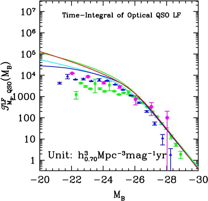
Figure 2.— The time integral of the QSO luminosity function in the optical band ($B$). The solid triangles (blue), solid circles (magenta) and solid squares (green) represent the direct summation of the binned QSO LF (eq. 13) obtained from Croom et al. (2004) over the redshift range $0.35<z<2.1$, Wolf et al. (2003) over the redshift range $1.2<z<4.8$ and Richards et al. (2006a) over the redshift range $0.3<z<5.0$, respectively. High-luminosity QSOs are under-represented in Croom et al. (2004) because of the redshift limit ($z<2.1$) and low-luminosity QSOs are under-represented in the sample in Richards et al. (2006a) because of incompleteness at the faint end (especially at high redshift). The blue, cyan, red, and green lines represent the time integrals obtained from the fitting formulae in Croom et al. (2004), Jiang et al. (2006), Boyle et al. (2000), and Richards et al. (2005), respectively. The time integrals obtained from different fitting formulae are consistent at the high-luminosity end but show substantial discrepancies at the low-luminosity end ($M_{\rm B}>-23$) mainly because of the uncertainties in the faint-end slope of the QSO LF. For example, the faint-end slope is estimated to be $\sim 1.09$ by Croom et al. (2004), $\sim 1.25$ in Jiang et al. (2006), but $\sim 1.58$ by Boyle et al. (2000) and $\sim 1.45$ by Richards et al. (2005). See also in Fig. 3.

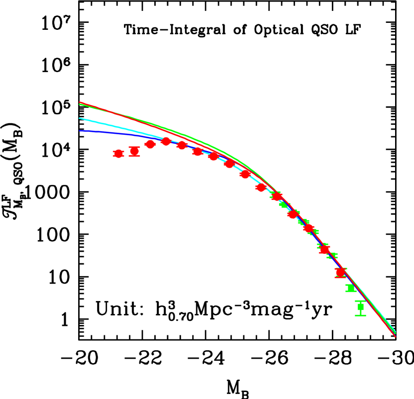
Figure 3.— The time integral of the QSO LF in the optical band ($B$). Similar to Fig. 2, but the points are obtained by combining the binned optical LFs given by different surveys over different redshift and luminosity ranges. At each redshift bin with data available, the binned optical LFs obtained from the largest sample are adopted, and interpolations of the data points over magnitudes at a given redshift are used. The points, which should be lower limits to the time integrals of the QSO LF, are quite consistent with that obtained from the fitting formulae of the QSO LF at $M_{\rm B}<-24$ (solid lines). At the faint end, the direct summations are substantially smaller than those estimated from the continuous fitting formulae with extrapolations to higher redshift and lower luminosities (which may be due to the incompleteness of the samples). The five green squares represent the brightest QSOs obtained from Richards et al. (2006a) only and they are consistent with the trend of the red points. The blue, cyan, red and green lines represent the time-integrals obtained from the fitting formulae in Croom et al. (2004), Jiang et al. (2006), Boyle et al. (2000) and Richards et al. (2005), respectively.

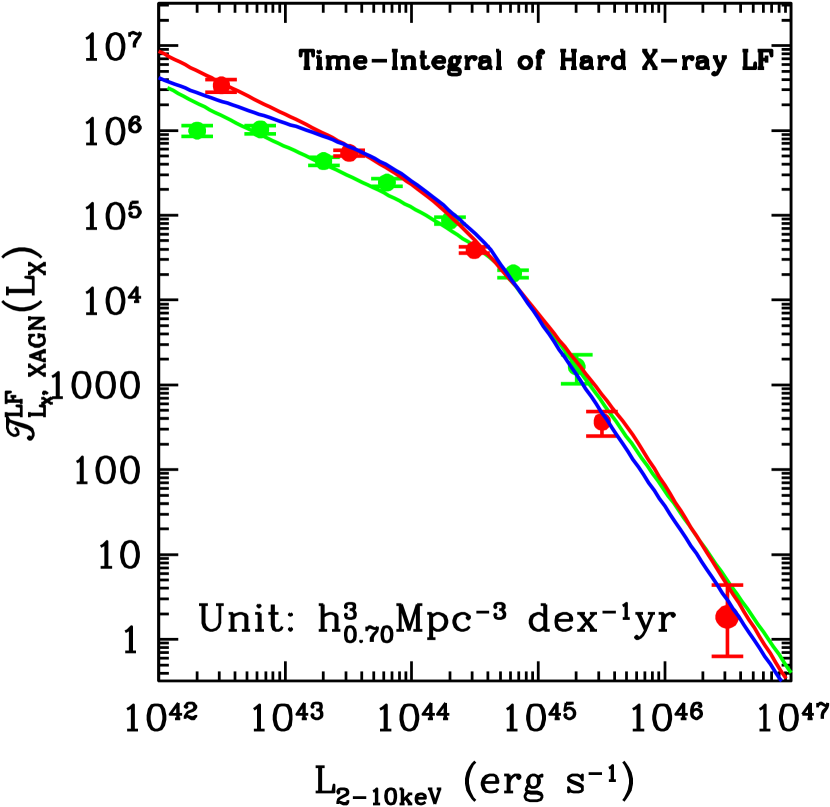
Figure 4.— The time integral of the X-ray AGN LF. The red solid circles represent the direct summations of the binned X-ray LF for the AGN sample over redshift range $0<z<2.5$ collected in La Franca et al. (2005), while the green solid circles represent the direct summations of the binned X-ray LF obtained from the AGN sample over redshift range $0.2<z<5.5$ by surveys such as the Chandra Deep Field (CDF) described in Silverman et al. (2008, see details in § 3). For the low-luminosity points, the sample may be incomplete at high redshifts and thus those points may be only lower limits, especially for the sample in Silverman et al. (2008) which may suffer from a bias due to the optical magnitude limits in the survey. The red, blue, and green lines represent the time integrals of the X-ray LFs in the redshift range $0<z<8$ according to the fitting formulae obtained by La Franca et al. (2005), Ueda et al. (2003), and Silverman et al. (2008), respectively. At the high-luminosity end ($L_{X}>10^{44}\rm erg~{}s^{-1}$), the time integrals are quite consistent with the binned data and with each other, but at the low-luminosity end ($L_{\rm X}<10^{43}\rm erg~{}s^{-1}$), the one obtained from Silverman et al. (2008) is smaller than that from La Franca et al. (2005) by a factor of $\gtrsim 2$. The estimates obtained from La Franca et al. (2005) at the low-luminosity end ($L_{X}\lesssim 10^{43.5}\rm erg~{}s^{-1}$) is taken as the best one, while at middle and high luminosities both the estimates from La Franca et al. (2005) and Silverman et al. (2008) are taken into account. Compton-thick sources, which are hard to be observed even in the X-ray, are not included (for the contribution of the Compton-thick AGNs to the time-integral of X-ray luminosity function see discussions in § 3.2).

3.3. The BC in the optical and hard X-ray bands

The BC of a QSO is usually defined by $C_{\nu}\equiv L_{\rm bol}/(\nu L_{\nu})$, where $\nu L_{\nu}$ is the energy radiated at the central frequency $\nu$ of a specific band. Based on observations from optical to hard X-rays, Elvis et al. (1994) constructed the spectral energy distributions (SEDs) for several tens of QSOs and estimated the BC in the $B$ band, which is about $11.8\pm 4.3$. Considering that the infrared bump in the Elvis et al.’s SED templates was probably due to reprocessing of UV to X-ray photons by the dusty torus rather than the intrinsic emission from the central nuclei, Marconi et al. (2004) obtained that the BC at the $B$ band is $7.9\pm 2.9$. Based mainly on an anti-correlation between the optical-to-X-ray spectral index ($\alpha_{ox}$) and the 2500Å luminosity (e.g., Vignali et al., 2003; Strateva et al., 2005; Steffen et al., 2006), Marconi et al. (2004) and Hopkins et al. (2007a) re-calibrated the SED and argued that the BC is luminosity-dependent. The BCs were derived by Marconi et al. (2004) as

$$\log[L_{\rm bol}/L_{2-10~{}{\rm keV}}]=1.54+0.24{\sf L}+0.012{\sf L}^{2}-0.0015{\sf L}^{3},$$ (20)

$$\log[L_{\rm bol}/\nu_{\rm B}L_{\nu_{\rm B}}]=0.80-0.067{\sf L}+0.017{\sf L}^{2}-0.0023{\sf L}^{3},$$ (21)

where ${\sf L}\equiv\log L_{\rm bol}-12$ and $L_{\rm bol}$ is the bolometric luminosity in units of $L_{\sun}$. Hopkins et al. (2007a) found

$$\frac{L_{\rm bol}}{L_{\rm band}}=c_{1}\left(\frac{L_{\rm bol}}{10^{10}L_{\sun}}\right)^{k_{1}}+c_{2}\left(\frac{L_{\rm bol}}{10^{10}L_{\sun}}\right)^{k_{2}},$$ (22)

with ($c_{1},k_{1},c_{2},k_{2}$) given by (6.25, -0.37, 9.00, -0.012) for $L_{\rm band}=L_{\rm B}$ and (10.83, 0.28, 6.08, -0.020) for $L_{\rm band}=L_{2-10~{}{\rm keV}}$. The scatter in BCs given by equation (22) is

$$\sigma_{\log(L_{\rm bol}/L_{\rm band})}=\sigma_{1}(L_{\rm bol}/10^{9}L_{\sun})^{\beta}+\sigma_{2},$$ (23)

where ($\sigma_{1}$, $\beta$, $\sigma_{2}$)=($0.08$, $-0.25$, $0.06$) in the $B$ band and ($0.06$, $0.10$, $0.08$) in the hard X-ray. The BC in hard X-ray given by Hopkins et al. (2007a) is $30\%$ larger than that given by Marconi et al. (2004), and the BC in the $B$ band given by Marconi et al. (2004) is smaller than that given by Hopkins et al. (2007a) by a factor of $1.5$ (or $1.8$) at $L_{\rm bol}=10^{10}L_{\sun}$ (or $L_{\rm bol}=10^{14}L_{\sun}$). In this paper, we adopt the BCs for the X-ray and $B$ bands and associated scatters obtained by Hopkins et al. (2007a). If the BCs given by Marconi et al. (2004) were adopted, the efficiency $\epsilon$ should be systematically smaller than that obtained below in § 4 by a factor of $\sim 1.3$ in order to match the time-integral of QSO/AGN LF obtained from observations with that inferred from the local BHMF.

We note that Vasudevan & Fabian (2007) recently investigated the SEDs of 54 AGN and found significant spreads in the BCs. Their results suggest a relationship between BCs in the X-ray band and Eddington ratios (see definition in § 4) in AGNs, with a transition at an Eddington ratio of $\sim 0.1$, below which the BC is typically $15-25$ for the $2-10$ keV luminosities and above which the BC is typically $40-70$. Their estimates of the BC for the optical band is approximately independent of Eddington ratio and roughly consistent with that obtained by Hopkins et al. (2007a). We also note that simple theoretical expectations of the BCs would be that it is not only the functions of Eddington ratios but also the functions of MBH masses because the SED of the disk emission depends on the MBH mass and Eddington ratio. In addition, the QSO/AGN variability in the hard X-ray is substantial while it is not significant in the optical band. The X-ray variability, typically a factor of $\sim 1.5$, introduces an additional scatter of $\sim 0.13$ dex to the BC for the hard X-ray band (see Tab. 2 in Vasudevan & Fabian, 2007). Since a quantitative relation between the BCs and the Eddington ratio is still premature, we shall not consider the BCs as functions of the Eddington ratio in this work but simply adopt equations (22) and (23) and include an additional scatter due to the X-ray variability.

The time integral of the QSO LF at any given wave-band $Y$ can also be inferred from the local BHMF as follows, provided that the BC at this band is known,

$${\cal T}^{\rm mod}_{Y,XAGN} = \int^{\infty}_{0}dL_{\rm bol}\int^{\infty}_{0}n_{M_{\bullet}}(M_{\bullet,0},t_{0})\tau_{\rm lt}(M_{\bullet,0})$$ (24)

$$P(L_{\rm bol}|M_{\bullet,0})P(L_{Y}|L_{\rm bol})dM_{\bullet,0},$$

where $L_{Y}$ is the luminosity at the Y-band, and $P(L_{Y}|L_{\rm bol})$ is the probability distribution of Y-band luminosity for QSOs/AGNs with bolometric luminosity $L_{\rm bol}$ and is determined by the BCs and their scatters.

4. Simple models for the luminosity evolution of individual QSOs

In this section, we introduce three simple models for the luminosity/accretion rate evolution of individual QSOs. These models are assumed to represent the luminosity/accretion rate evolution averaged over an intermediate timescale substantially smaller than the lifetime of individual QSOs, but much longer than certain details of the evolution such as the short time variation, etc. The parameters involved in these models will then be constrained by observations of the local BHMF and the QSO/AGN LF through the extended Sołtan argument (eq. 1). Because X-ray surveys are more complete than optical surveys in the sense that obscured AGN can be detected in X-ray surveys, we will compare the time integrals obtained from the X-ray LF with that inferred from the local BHMF in this section, and then use the time integral of the optical QSO LF to give constraints on obscured AGN fraction in the optical band in § 5.

4.1. Several fiducial parameters

We first summarize several fiducial parameters involved in the models below.

• The “Eddington luminosity” is a characteristic luminosity at which radiation pressure on free electrons balances gravity:

  $$L_{\rm Edd}(M_{\bullet}) = \frac{4\pi GM_{\bullet}m_{\rm p}c}{\sigma_{\rm T}}$$ (25)

  $$\simeq 1.26\times 10^{46}\left(\frac{M_{\bullet}}{10^{8}M_{\odot}}\right){\rm erg~{}s^{-1}},$$

  where $G$ is the gravitational constant, $m_{\rm p}$ is the mass of a proton, and $\sigma_{\rm T}$ is the cross-section of Thompson scattering. The Eddington luminosity is frequently assumed to be the maximum luminosity of any object of mass $M_{\bullet}$.

• Corresponding to the Eddington luminosity, the “Eddington accretion rate” is defined by:

  $$\dot{M}^{\infty}_{\rm acc,Edd} \equiv \frac{L_{\rm Edd}}{\epsilon c^{2}}$$ (26)

  $$= 2.22\left(\frac{0.1}{\epsilon}\right)\left(\frac{M_{\bullet}}{10^{8}M_{\odot}}\right)M_{\odot}\rm yr^{-1},$$

  where $\epsilon$ is the mass-to-energy conversion efficiency; and the Eddington growth rate of a MBH is

  $$\dot{M}_{\bullet,\rm Edd}=(1-\epsilon)\dot{M}^{\infty}_{\rm acc,Edd}.$$ (27)

  The efficiency $\epsilon$ is predicted to be in the range $\sim 0.04-0.31$ in the thin disk accretion models, depending on the spin of the MBH [$\epsilon=0.057$ for a Schwarzschild BH, and $0.31$ ($0.04$) for a prograde (retrograde) rotating accretion disk around a Kerr BH with the dimensionless spin parameter $a\sim 0.998$, the upper limit of BH spin if the BH is spun up by accretion; Thorne 1974]. Currently, the spin of MBHs is difficult to measure directly. Theoretical studies of the spin evolution of MBHs show that MBH spin may reach an equilibrium point for most of its lifetime considering both accretion and merger processes (e.g., Lu et al., 1996; Gammie et al., 2004; Shapiro, 2005; Volonteri et al., 2005; Hawley et al., 2007; Noble et al., 2008; Hughes & Blandford, 2003). This equilibrium value is $\sim 0.7-0.9$ and corresponds to an efficiency $\epsilon\sim 0.10-0.20$ (e.g., Gammie et al., 2004; Shapiro, 2005; Hawley et al., 2007). If the accretion rate of a MBH is less than the Eddington rate by a factor much larger than $100$ (e.g., $\dot{m}\equiv\dot{M_{\bullet}}/\dot{M_{\bullet}}_{\rm,Edd}\lesssim 10^{-3}$), the MBH may accrete material via the Advection Dominated Accretion Flow (ADAF) with very low efficiency, $\epsilon\ll 0.1$ (e.g., Narayan & Yi 1994), or via a mode described by the Advection Dominated Inflow and Outflow scenario (ADIOS, Blandford & Begelman 1999) with most of the accretion material blown away. The contribution from these very low efficiency modes to the observational range of the time integral of the QSO/AGN LF is negligible and MBH growth may also be very inefficient in this low-accretion rate mode. In this paper, we will not consider this complication but assume that $\epsilon$ is a constant that is neither directly nor indirectly related to the BH mass $M_{\bullet}$ and the accretion rate, as $\epsilon$ is probably mainly determined by the spin of the central BH in the thin-disk accretion mode. (A more detailed study of the growth of MBHs should simultaneously consider the spin and mass evolution of MBHs.)

• If a MBH-disk accretion system accretes material via the Eddington accretion rate and radiates with luminosity $L_{\rm bol}$, the mass of the MBH is

  $${M_{\bullet}}_{,\rm Edd}(L_{\rm bol})=\left(\frac{L_{\rm bol}}{1.26\times 10^{38}\rm erg~{}s^{-1}}\right)M_{\odot}.$$ (28)

• The Salpeter timescale is defined as the time for a MBH radiating at the Eddington luminosity to e-fold in its mass:

  $$\tau_{\rm S}\equiv\frac{M_{\bullet}}{\dot{M}_{\bullet,{\rm Edd}}}=4.5\times 10^{7}\frac{\epsilon}{0.1(1-\epsilon)}\rm yr.$$ (29)

  If the accretion rate is only a fraction $\lambda$ of the Eddington accretion rate, then the timescale for a MBH to e-fold its mass is $\tau_{\rm S}^{\prime}=\lambda^{-1}\tau_{\rm S}$.

4.2. Model (a)

The mass of MBHs in QSOs may be estimated by using the virial mass estimator(s), i.e., using the width of broad emission lines and the empirical relation between the optical luminosities and the sizes of broad line regions estimated from reverberation mapping studies (e.g., Wandel, Peterson & Malkan 1999; Kaspi et al. 2000; Vestergaard 2002; Kaspi et al. 2005; see also discussion of uncertainties, e.g., in Krolik 2001), and hence the Eddington ratio may be estimated (e.g., Woo & Urry, 2002). Recent studies by Kollmeier et al. (2006) on a sample of QSOs using the virial mass estimator(s) have suggested that the Eddington ratios ($\dot{m}=L_{\rm bol}/L_{\rm Edd}$) in QSOs, may be consistent with a single value, and the best estimates of the mean value of $\dot{m}$ is around $10^{-0.6}$ for all redshifts and luminosities. Using a large sample of QSOs from SDSS, Shen et al. (2007) investigate the Eddington ratio distribution in QSOs over a range of redshifts and luminosities, however, their results show that the mean value of the Eddington ratio is a function of redshift and luminosity and it ranges from $10^{-1.1}$ and $10^{-0.6}$. Netzer et al. (2007) also argue that the $\dot{m}$ distribution is not consistent with a single value and the conclusion that a single $\dot{m}$ applies to all QSOs/AGNs might be due to some unknown selection effects. Ignoring this concern, for the moment, we assume that all MBHs in QSOs accrete material at a constant normalized rate $\dot{m}=\lambda$, i.e., $\dot{M_{\bullet}}=\lambda\dot{M_{\bullet}}_{\rm,Edd}$ while the QSO is “on”. The luminosity evolution is

$$L_{\rm bol}(M_{\bullet,0},\tau) = \lambda L_{\rm Edd}(M_{\bullet,0})\exp\left[\frac{\tau-\tau_{\rm lt}(M_{\bullet,0})}{\tau_{\rm S}^{\prime}}\right],$$ (30)

$$\qquad{\rm for\ \ \ }0<\tau<\tau_{\rm lt}(M_{\bullet,0}).$$

This model involves three parameters $(\epsilon,\lambda,\xi)$, where $\xi=\tau_{\rm lt}(M_{\bullet,0})/\tau_{\rm S}^{\prime}=\lambda\tau_{\rm lt}(M_{\bullet,0})/\tau_{\rm S}$; and these three parameters solely determine the growth history of individual MBHs. For MBHs with present-day mass $M_{\bullet,0}$, the probability distribution of the nuclear luminosity in their evolutionary history (eq. 3) is

$$P(L_{\rm bol}|M_{\bullet,0})=\frac{f_{Q}}{\xi}\frac{1}{L_{\rm bol}},$$ (31)

where

$$f_{Q}=\cases{1&if $\frac{{M_{\bullet}}_{,\rm Edd}(L_{\rm bol})}{\lambda}\leq M_{\bullet,0}\leq\frac{{M_{\bullet}}_{,\rm Edd}(L_{\rm bol})}{\lambda}\exp(\xi)$,\cr 0&otherwise,}$$ (32)

and the present-day mass of a MBH is related to its initial mass $M_{\bullet,i}$ at the time of nuclear activity being triggered by $M_{\bullet,0}=M_{\bullet,i}\exp(\xi)$.

For a given set of parameters $(\epsilon,\lambda,\xi)$, we calculate the time integrals of the XAGN LF, ${\cal T}_{L_{X},\rm XAGN}^{\rm mod}$ (or ${\cal T}_{M_{\rm B},\rm XAGN}^{\rm mod}$), using equation (24). To do this, the local BHMF is chosen to be the one estimated by using the $M_{\bullet,0}-\sigma$ relation by Lauer et al. (2007a) as the reference BHMF in this paper (see the solid blue line in the right bottom panel of Fig 1). For given BHMF, BCs, and $\lambda$, the normalization of the inferred time integrals of XAGN LF, i.e., ${\cal T}_{L_{X},\rm XAGN}^{\rm mod}$, is proportional to $\epsilon/(1-\epsilon)$ through $\tau^{\prime}_{S}$, which can vary by a factor of 10 for the typical range of $\epsilon$, 0.04–0.31. If $\xi$ is substantially smaller than 1, ${\cal T}_{L_{X},\rm XAGN}^{\rm mod}$ is also proportional to $\xi$ because the range of the integration limits over the BH mass is quite small and thus approximately proportional to $\xi$, and the shape of the inferred time integrals of the QSO LF is determined by the shape of the local BHMF. In this case, there is some degeneracy between the parameters $\xi$ and $\epsilon$ if $\xi<1$. However, this degeneracy does not exist if $\xi$ is substantially larger than 1 (i.e., if the growth of MBHs is dominated by accretion processes) [which is also true for models (b) and (c) below], as ${\cal T}_{L_{X},\rm XAGN}^{\rm mod}$ is insensitive to $\xi$ at the high-luminosity end and increases only slowly with increasing $\xi$ at the low-luminosity end. For example, the predicted ${\cal T}_{L_{X},\rm XAGN}^{\rm mod}$ for the case of $\xi=2$ (but fixed $\epsilon$ and $\lambda$) at the low-luminosity end ($L_{X}\lesssim 10^{43}\rm erg~{}s^{-1}$) is smaller than that for the case of $\xi=10$ (with the same $\epsilon$ and $\lambda$) by a factor of $\sim 1.2-1.3$, and ${\cal T}_{L_{X},\rm XAGN}^{\rm mod}$ for these two cases are almost the same at the high-luminosity end ($L_{X}\gtrsim 10^{44}\rm erg~{}s^{-1}$).

As shown in Figure 5, $\lambda$ should be in the range from 0.5 to 1 in order to match the observations at high luminosity ($L_{\rm X}>10^{44}\rm erg~{}s^{-1}$) with ${\cal T}_{L_{X},\rm XAGN}^{\rm mod}$, while it should be close to $0.1$ in order to match the observations at lower luminosities ($L_{X}<10^{43.5}\rm erg~{}s^{-1}$). According to Figure 5, we conclude that the inferred time integrals of the XAGN LF cannot match the observations at both the low-luminosity and the high-luminosity ends simultaneously if all MBHs accrete material at a single $\dot{m}=\lambda$.

We should note here that ${\cal T}_{L_{X},\rm XAGN}^{\rm mod}$ may well fit the observations if $\lambda$ is arbitrarily assumed to be an increasing function of $M_{\bullet,0}$ (cf., the Eddington ratio may be redshift-dependent and thus mass-dependent since statistically MBHs with larger $M_{\bullet,0}$ formed earlier, see Shankar et al. 2004, 2007). However, the assumption that all low-mass MBHs need to accrete material via lower Eddington ratios may be not realistic/physical because (1) some low-mass MBHs, such as the one in NGC 3079 (with MBH mass $\sim 2\times 10^{6}M_{\odot}$) or NGC 1068 (with MBH mass $\sim 8\times 10^{6}M_{\odot}$), do accrete material with a rate close to the Eddington limit and have massive accretion disks with mass comparable to the MBH mass (Kondratko et al., 2005; Lodato & Bertin, 2003); and (2) there is no clear physical reason for the low-mass MBHs to accrete material via smaller Eddington ratios compared to high-mass MBHs if they also obtained their mass mainly from accretion. Therefore, we do not pursue the possibility that the Eddington ratio is constant for each AGN with the same MBH mass but an increasing function of the MBH mass.

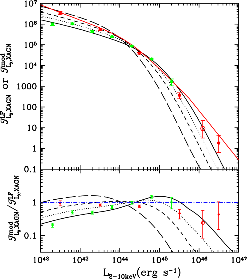
Figure 5.— Comparison of the time integral of the X-ray AGN luminosity function (XAGN LF) and that inferred from the local BHMF by adopting model (a) in § 4, i.e., assuming that all MBHs accrete material via a fixed Eddington ratio ($\lambda$). The symbols and the red line are the same as in Fig. 4. The black lines represent the inferred time integrals of the XAGN LF from the local BHMF with $\epsilon=0.14$, $\xi=10$, and $\lambda=1$ (solid line), 0.5 (dotted line), 0.25 (short-dashed line), and 0.08 (long-dashed line), respectively. The bottom panel shows the inferred time integrals of the XAGN LF from the BHMF compared to the prediction of the fitting-formula of XAGN LF obtained by La Franca et al. (2005). Note that the estimate of the highest-luminosity point at $L_{X}=10^{46.5}\rm erg~{}s^{-1}$ cannot fit into any model, which might be partly because this point is estimated in La Franca et al. (2005) from only two AGN with luminosity $\sim 10^{46.1}\rm erg~{}s^{-1}$ in the bin $10^{46}-10^{47}\rm erg~{}s^{-1}$. We use these two AGNs to give an estimate on the space density of AGN at $\sim 10^{46.1}\rm erg~{}s^{-1}$ in a bin $10^{46}-10^{46.2}\rm erg~{}s^{-1}$ and show it as the open circle in this figure. The estimates obtained from La Franca et al. (2005) at the low-luminosity end ($L_{\rm X}\lesssim 10^{43.5}\rm erg~{}s^{-1}$, the red points) are adopted as the best one since the low-luminosity data from Silverman et al. (2008) may suffer from selection bias, while at middle- and high-luminosities ($10^{43.5}\rm erg~{}s^{-1}<L_{X}<10^{46}\rm erg~{}s^{-1}$, the green points) both the estimates from La Franca et al. (2005) and Silverman et al. (2008) are taken into account. As shown in this Figure, the inferred time-integrals of XAGN LF cannot match the observations simultaneously at both the low-luminosity and high-luminosity ends.

4.3. Model (b)

A more realistic model would be that the growth of MBHs involves two phases after the nuclear activity is triggered (see the discussions in Small & Blandford 1992, Blandford 2003, and Yu & Lu 2004a). In the first phase, there is plenty of material to supply the MBH growth; however, MBHs may not be able to accrete as fast as material fueling allows because the accretion process may be self-regulated by the Eddington limit. With the decline of the material supply, the MBH growth enters the second phase and the nuclear luminosity in which the limiting factor is the fuel supply and accretion rate are expected to decline to below the Eddington limit.

After the nuclear activity of a MBH is triggered at cosmic time $t_{i}$, we assume that the MBH accretes material via the Eddington accretion rate for a time-period of $\tau_{P}=\xi\tau_{\rm S}$, hence its mass increases to $M_{\bullet,{P}}$ and its luminosity approaches a peak of $L_{P}(M_{\bullet,0})=L_{\rm Edd}(M_{\bullet,{P}})$ at time $t_{P}=t_{i}+\tau_{P}$. The nuclear luminosity in this phase increases with time as

$${L}_{\rm bol}(\tau)=L_{\rm Edd}(M_{\bullet,{P}})\exp\left(\frac{\tau-\tau_{P}}{\tau_{\rm S}}\right),\qquad 0<\tau<\tau_{P},$$ (33)

where $\tau=t-t_{i}$ is the age of the QSO since the nuclear activity was triggered.

In the second phase, we assume that the evolution of the nuclear luminosity (or accretion rate) declines exponentially as (e.g., Haehnelt et al. 1998; Haiman & Loeb 1998):

$${L}_{\rm bol}(M_{\bullet,0},\tau)=$$

$$\cases{L_{\rm Edd}(M_{\bullet,{P}})\exp\left(-\frac{\tau-\tau_{P}}{\tau_{D}}\right),&for $\tau_{P}\leq\tau\leq\tau_{P}+\eta\tau_{D}$,\cr 0,&for $\tau>\tau_{P}+\eta\tau_{D}$,}$$

(34)

where $\tau_{D}=\zeta\tau_{\rm S}$ is the characteristic decay timescale of the nuclear luminosity. We assume that QSOs become quiescent when the nuclear luminosity declines by a factor of $\exp(-\eta)$ compared to the peak luminosity $L_{\rm Edd}(M_{\bullet,{P}})$, so there is a cutoff of the nuclear luminosity at $\tau_{\rm lt}=\tau_{P}+\eta\tau_{D}=(\xi+\eta\zeta)\tau_{\rm S}$ in equation (34). The factor $\eta$ is set to $-\ln(10^{-3})=6.9$ here, since after decreasing by a factor of $10^{-3}$ in accretion rate, the accretion mode may change from the efficient thin-disk accretion to the inefficient advection dominated accretion modes and the nuclear luminosity of MBHs even with a high mass $\sim 10^{9}M_{\odot}$ will become fainter than the luminosity range ($M_{\rm B}\lesssim-20$ or $L_{X}\lesssim 10^{42}\rm erg~{}s^{-1}$) of interest in this paper. With the assumption that all QSOs are quenched at present (i.e., $t_{0}-t_{i}-\tau_{P}\gg\tau_{D}$), the MBH mass at the present day is

$$M_{\bullet,0}\simeq\left(1+\zeta\right)M_{\bullet,{P}}=(1+\zeta)\exp(\xi)M_{\bullet,i}.$$ (35)

This model reduces to model (a) with $\lambda=1$ if the second phase is not significant.

For MBHs with present-day mass $M_{\bullet,0}$, the probability distribution of the nuclear bolometric luminosity in their evolutionary history (eq. 3) is

$$P(L_{\rm bol}|M_{\bullet,0})=\frac{f_{P}+\zeta f_{D}}{\xi+\eta\zeta}\frac{1}{L_{\rm bol}},\qquad$$ (36)

where

$$f_{P}=\\ \cases{1&if $(1+\zeta){M_{\bullet}}_{,\rm Edd}(L_{\rm bol})\leq M_{\bullet,0}\leq$\cr&\qquad$(1+\zeta)\exp(\xi){M_{\bullet}}_{,\rm Edd}(L_{\rm bol})$,\cr 0&otherwise,}$$

and

$$f_{D}=\cases{1&if $(1+\zeta){M_{\bullet}}_{,\rm Edd}(L_{\rm bol})\leq M_{\bullet,0}\leq$\cr&\qquad$10^{3}(1+\zeta){M_{\bullet}}_{,\rm Edd}(L_{\rm bol})$,\cr 0&otherwise.}$$ (37)

In model (b), we also have three parameters $(\epsilon,\xi,\zeta)$ to be constrained below.

For any given set of parameters ($\epsilon$, $\xi$, $\zeta$), we calculate the time integrals of the XAGN LF, ${\cal T}^{\rm mod}_{L_{X},\rm XAGN}$. Our calculations show that the dependence of ${\cal T}^{\rm mod}_{L_{X},\rm XAGN}$ on parameters $\epsilon$ or $\xi$ for a given $\zeta$ is similar to that in model (a). For given $\epsilon$ and $\xi$, a larger $\zeta$ corresponds to smaller ${\cal T}^{\rm mod}_{L_{X},\rm XAGN}$ at higher luminosities but larger ${\cal T}^{\rm mod}_{L_{X},\rm XAGN}$ at lower luminosities. As shown in Figure 6, $\zeta$ must be around or smaller than $0.1-0.3$ to match ${\cal T}^{\rm mod}_{L_{X},\rm XAGN}$ with observations at the high-luminosity end ($L_{X}\gtrsim 10^{44.5}\rm erg~{}s^{-1}$), but $\zeta$ should be larger than $1$ to match ${\cal T}^{\rm mod}_{L_{X},\rm XAGN}$ with observations at the low-luminosity end ($L_{X}\lesssim 10^{43}\rm erg~{}s^{-1}$). It is unlikely that ${\cal T}^{\rm mod}_{L_{X},\rm XAGN}$ inferred from any single $\zeta$ with any fixed ($\epsilon$, $\xi$) can match observations simultaneously at both the high- and low-luminosity end.

As discussed in model (a), $\xi$ and $\zeta$ are not necessarily constants in model (b) but may be functions of $M_{\bullet,0}$; or alternatively the ratio of the MBH mass $M_{\bullet,{P}}$ at the peak luminosity to the final MBH mass $M_{\bullet,0}$ may be a slowly increasing function of $M_{\bullet,0}$ as proposed by Hopkins et al. (2006). The dependence of $\xi$ and $\zeta$ on $M_{\bullet,0}$ would be related to the assembly history of each MBH and the distribution of seed BHs, which are poorly known. In model (b), it is possible that ${\cal T}^{\rm mod}_{L_{X},\rm XAGN}$ can match observations at both the high- and low-luminosity ends if $\zeta$ decreases with increasing $M_{\bullet,0}$. But we will not go further to make this fit, for the same reasons given at the end of § 4.2.

Figure 6.— Similar to Fig. 5, but adopting model (b) in § 4, i.e., an initial accretion phase with rate set by the Eddington limit, followed by a phase with an exponentially declining accretion rate. The black lines represent the inferred time integrals of XAGN LF from the local BHMF with $\epsilon=0.16$, $\xi=10$, and $\zeta=0.1$ (long-dashed line), 0.3 (short-dashed line), 1 (dotted line) and 3 (solid line), respectively. As shown in this Figure, the inferred time-integrals of XAGN LF cannot match the observations simultaneously at both the low-luminosity and high-luminosity ends.

4.4. Model (c)

The accretion rates in the second phase of QSOs, in which the luminosity decays, may be ultimately determined by the evolution of the viscous accretion disk itself rather than galactic-scale dynamical disturbances. The disk accretion evolution may follow a self-similar solution (e.g., Pringle, 1981; Lin & Pringle, 1987; Cannizzo et al., 1990; Pringle, 1991), i.e., the accretion rate declines as a power-law of the QSO age ($\dot{M_{\bullet}}\propto\tau^{-\gamma}$), where the slope $\gamma$ may be determined by the opacity law. The value of $\gamma$ also depends on the binarity of the MBH surrounded by the accretion disk, for instance, $\gamma\sim 1.2-1.3$ for the evolution of a disk around a single MBH (e.g., Cannizzo et al., 1990), while $\gamma\sim 2.5-3.3$ for a disk truncated by an outer secondary MBH (e.g., Lipunova & Shakura, 2000). For the binary MBH system, however, the secondary MBH embedded in a disk surrounding the primary MBH may migrate inward and may merge with the primary MBH on a time-scale of $10^{7}$ yr (e.g., Armitage & Natarajan, 2002; Escala et al., 2004, 2005), and thus the evolution of disk accretion associated with the binary MBH system ($\gamma\sim 2.5-3.3$) may not be sustained for a period substantially longer than $10^{7}$ yr. The observed accretion rate distribution in local AGNs is found to be consistent with the self-similar evolution around a single MBH and $\gamma\simeq 1.26\pm 0.1$ (Yu et al., 2005, see also King & Pringle 2007b). In this paper we neglect the complications in the evolution of disk accretion due to possible binary MBHs, and assume $\gamma\sim 1.2-1.3$. Below we introduce model (c) which is similar to model (b) but the nuclear luminosity in the second phase declines with time as a power law:

$${L}_{\rm bol}(M_{\bullet,0},\tau)=$$

$$\cases{L_{\rm Edd}(M_{\bullet,{P}})\left(\frac{\tau+\tau_{D}-\tau_{P}}{\tau_{D}}\right)^{-\gamma},&for $\tau_{P}\leq\tau\leq\tau_{P}+\eta\tau_{D}$,\cr 0,&for $\tau>\tau_{P}+\eta\tau_{D}$,}$$

(38)

where $\tau_{D}=\zeta\tau_{\rm S}$ is the transition timescale from the first to the second phase. As in model (b), we assume that QSOs become quiescent when the nuclear luminosity declines by a factor of $10^{3}$ compared to the peak luminosity $L_{\rm Edd}(M_{\bullet,{P}})$ and afterwards the growth of MBHs is not significant. Thus $\eta=10^{3/\gamma}-1$ in this model. The MBH mass at a time $\tau$ after the nuclear activity was triggered is

$$M_{\bullet}^{\tau}=M_{\bullet,{P}}\exp\left(\frac{\tau-\tau_{P}}{\tau_{\rm S}}\right),$$ (39)

in the first phase, and is

$$M_{\bullet}^{\tau}=M_{\bullet,{P}}\left[1+\frac{\zeta}{\gamma-1}\left(1-(\frac{\tau+\tau_{D}-\tau_{P}}{\tau_{D}})^{1-\gamma}\right)\right]$$ (40)

in the declining phase. The present-day mass of a MBH is

$$M_{\bullet,0}\simeq\chi M_{\bullet,{P}}=\chi\exp(\xi)M_{\bullet,i},$$ (41)

where $\chi=1+\frac{1-10^{3(1-\gamma)/\gamma}}{\gamma-1}\zeta$. The slope can be $\gamma\sim 1.2$, $1.3$ and thus $M_{\bullet,0}\sim(1+3.41\zeta)M_{\bullet,{P}}$, and $(1+2.66\zeta)M_{\bullet,{P}}$, respectively.

In model (c), for MBHs with present-day mass $M_{\bullet,0}$ the probability distribution of the nuclear bolometric luminosity in their evolutionary history (eq. 3) is

$$P(L_{\rm bol}|M_{\bullet,0})=\frac{f_{P}+f_{D}\frac{\zeta}{\gamma}\left(\frac{L_{\rm Edd}(M_{\bullet,{P}})}{L_{\rm bol}}\right)^{1/\gamma}}{\xi+\eta\zeta}\frac{1}{L_{\rm bol}},\qquad$$ (42)

where

$$f_{P}=\cases{1&if $\chi{M_{\bullet}}_{,\rm Edd}(L_{\rm bol})\leq M_{\bullet,0}$\cr&\qquad$\leq\chi\exp(\xi){M_{\bullet}}_{,\rm Edd}(L_{\rm bol})$\cr 0&otherwise,}$$ (43)

and

$$f_{D}=\cases{1&if $\chi{M_{\bullet}}_{,\rm Edd}(L_{\rm bol})\leq M_{\bullet,0}\leq 10^{3}\chi{M_{\bullet}}_{,\rm Edd}(L_{\rm bol})$,\cr 0&otherwise.}$$ (44)

Besides the three parameters $(\epsilon,\xi,\zeta)$ involved in model (c), an additional parameter $\gamma$ is also involved, but $\gamma$ is fixed by assumption to be 1.2–1.3 here, if not otherwise specified, according to theoretical models on the long-term evolution of viscous disk (e.g., Pringle, 1981; Lin & Pringle, 1987; Cannizzo et al., 1990; Pringle, 1991) and recent observational constraints (e.g., Yu et al., 2005, see also King & Pringle 2007b).

For any given $\zeta$ in this model, the dependence of ${\cal T}^{\rm mod}_{L_{X},\rm XAGN}$ on the parameters $\epsilon$ and $\xi$ is similar to that in models (a) and (b). For given $\epsilon$ and $\xi$, a larger $\zeta$ is responsible for a smaller ${\cal T}^{\rm mod}_{L_{X},\rm XAGN}$ at higher luminosities but a larger ${\cal T}^{\rm mod}_{L_{X},\rm XAGN}$ at lower luminosities because a larger $\zeta$ means that a larger fraction of the mass of MBHs is accreted via the second phase with Eddington ratios (substantially) smaller than 1. Although the growth history of both low-mass MBHs and high-mass MBHs is assumed the same in this model for fixed parameters ($\epsilon$, $\xi$, $\zeta$), apparently there are more objects with low Eddington ratios at the low-luminosity end but few objects with low Eddington ratios at the high-luminosity end. Detailed investigation of the Eddington ratio distribution inferred from this model is discussed in § 6. As shown in Figure 7, ${\cal T}^{\rm mod}_{L_{X},\rm XAGN}$ can match observations very well if $\zeta\sim 0.15-0.3$ provided that $\epsilon=0.16$, $\xi\gtrsim 2$ and $\gamma\sim 1.2-1.3$. With the parameter $\zeta\sim 0.15-0.3$ and $\gamma\sim 1.2-1.3$, the mass growth of MBHs at the accretion stage with Eddington ratio $\dot{m}<1$ ( or $\dot{m}\lesssim 0.1$) is roughly a fraction $\sim 0.2-0.5$ (or $\sim 0.1-0.3$) of its final mass $M_{\bullet,0}$, and this is compatible with the assumption that the disk mass is substantially less than the central MBH in the long-term evolution of disk accretion model (e.g., Pringle, 1981; Lin & Pringle, 1987; Cannizzo et al., 1990; Pringle, 1991); and MBHs obtained majority of their mass ($\gtrsim 80\%$) via a rate close to the Eddington limit ($\dot{m}\gtrsim 0.1$). With these parameters, we have $\tau_{\rm lt}(M_{\bullet,0})\sim\tau_{\rm S}[\xi+(10^{3/\gamma}-1)\zeta]\sim(3-6)\times 10^{9}$ yr, and the period for MBH-accretion disk systems radiating at luminosities larger than $10\%$ of its peak luminosity, thus roughly $\dot{m}\gtrsim 0.1$ (or $\dot{m}\gtrsim 0.01$), is only about $(3-4)\tau_{\rm S}\sim(2-3)\times 10^{8}$ yr (or $\sim 10^{9}$ yr). Model (c) is based on detailed considerations of the evolution of disk accretion and appears to fit observations much better than models (a) and (b). Therefore, this model with three parameters ($\epsilon$, $\xi$, $\zeta$)=($0.16$, $10$, $0.20$) is set as the reference model in this paper.

Considering of the uncertainty in the $M_{\bullet,0}-\sigma$ relation, the velocity dispersion distribution function and the time integral of XAGN LF, the error in the best-matched parameter $\epsilon$ is $\delta\epsilon\sim 0.04$. Note also that Compton-thick objects may be still missed in the hard X-ray surveys by La Franca et al. (2005). The fraction of Compton-thick objects should not be larger than $30$% according to the X-ray background synthesis model (e.g., Müller & Hasinger, 2007), and this would add additional uncertainty at most ${}^{+0.05}_{-0}$ to $\epsilon$. To match the time integral of XAGN LF with the local BHMF, the efficiency $\epsilon$ is required to $\simeq 0.16\pm 0.04^{+0.05}_{-0}$, and this range of $\epsilon$ is fully consistent with theoretical expectations $\epsilon\sim 0.10-0.20$ (e.g., Gammie et al., 2004; Shapiro, 2005; Hawley et al., 2007). The range of $\epsilon$ ($\sim 0.12-0.25$) constrained above corresponds to the spin parameter $a$ in the range from $\sim 0.8$ to $0.99$ as the value of $\epsilon$ is mainly determined by $a$ with only an order of $10-20\%$ or less uncertainty (e.g., Noble et al. 2008), which suggests that most MBHs in QSOs are indeed rapidly rotating Kerr BHs. It is worth to note that if we choose $\epsilon=0.21$, the time integral of XAGN LF inferred from the local BHMF with parameters ($\xi\sim 1$, $\zeta\sim 0.2$) can still match the observations well, but the time integral of XAGN LF at luminosities $L_{X}\lesssim 10^{45}\rm erg~{}s^{-1}$ is overpredicted by $\sim 40\%$ if ($\xi\sim 10$, $\zeta\sim 0.2$) and the overpredicted part can be accounted for by the additional contribution from Compton-thick AGNs. Previous estimates of the efficiency include $\epsilon\gtrsim 0.15$ (Elvis et al., 2002), $\epsilon\gtrsim 0.1$ (Yu & Tremaine, 2002; Yu & Lu, 2004a), $\epsilon\sim 0.04-0.16$ (Marconi et al., 2004), $\epsilon\sim 0.30-0.35$ (Wang et al., 2006), and $\epsilon\sim 0.06-0.11$ (Shankar et al., 2004, 2007).

The relatively high efficiency constrained above suggests that the majority of QSOs should not accrete material via the chaotic accretion scenario proposed by King & Pringle (2007a) to explain the rapid growth of MBHs in those QSOs at $z>6$, in which MBHs spin down because of counter-alignments of their spin axes with accretion disk angular momenta and thus the efficiency reduces to a low value, close to the efficiency for Schwarzschild BHs.

Note that there are some uncertainties in the intrinsic scatter in the $M_{\bullet,0}-\sigma$ relation, which may mainly introduce some uncertainties to the parameter $\zeta$. A larger intrinsic scatter corresponds to more MBHs at the high-mass end and thus allows a larger $\zeta$. But the uncertainties in $\zeta$ introduced by the uncertainties in the intrinsic scatter is not significant if this uncertainty in the scatter is less than $0.1$ dex (for example, it is about $0.06$ dex in Tundo et al. 2007).

In the above models, we adopt the local BHMF estimated from the $M_{\bullet,0}-\sigma$ relation and the velocity-dispersion distribution function. Arguably the $M_{\bullet,0}-L_{\rm bulge}$ relation may be favored, at least for the most massive galaxies (see Lauer et al. 2007a, but Batcheldor et al. 2007 and Graham 2008). If we adopt the local BHMF estimated from the $M_{\bullet,0}-L_{\rm bulge}$ relation and the galaxy luminosity function without correction of the bias as discussed in § 2, the time integral of XAGN LF can be matched by ${\cal T}^{\rm mod}_{L_{X},\rm XAGN}$ inferred from the local BHMF if $\xi=10$, $\zeta\sim 0.15-0.3$ but $\epsilon\simeq 0.08\pm 0.02^{+0.03}_{-0}$ (correspondingly the spin parameter $a$ is in the range from $0.1$ to $0.8$); and therefore the QSO lifetime constrained here is smaller than that constrained by the local BHMF obtained from the $M_{\bullet,0}-\sigma$ relation by a factor $\sim 2$. This is primarily due to the fact that the shape of the local BHMF estimated from the $M_{\bullet,0}-L_{\rm bulge}$ relation is similar to that estimated from the $M_{\bullet,0}-\sigma$ relation except that the normalization differs by a factor close to $2$ (see discussions in § 2 and the bottom left panel of Fig. 1).

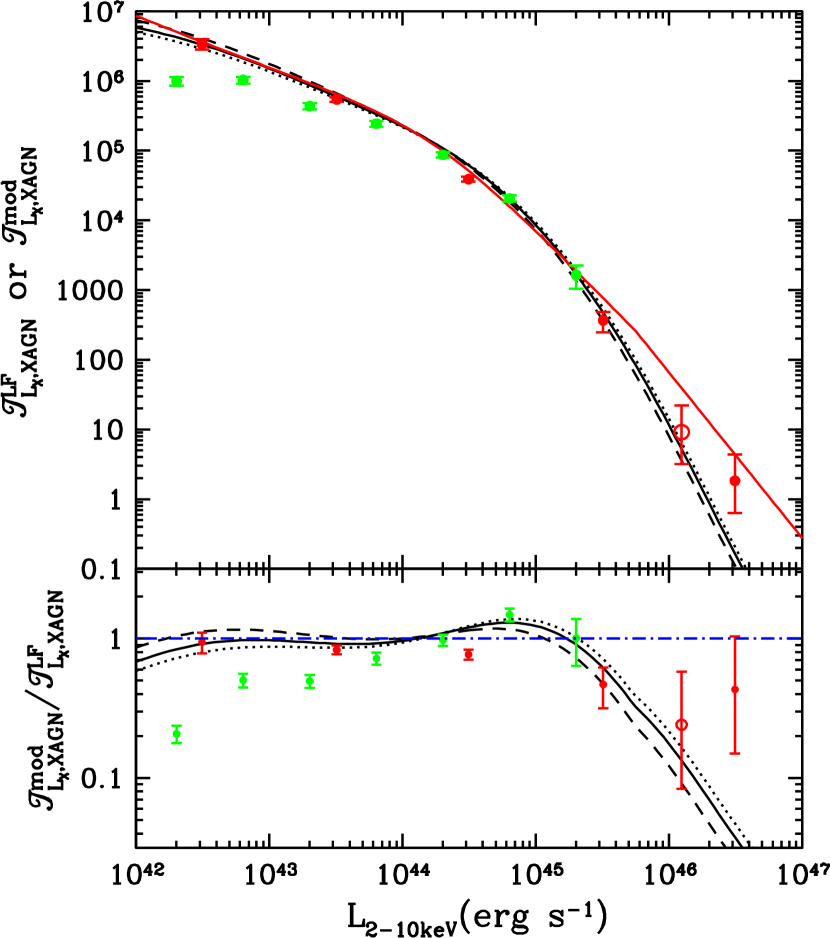
Figure 7.— Similar to Fig. 5, but adopting model (c) in § 4, i.e., an initial accretion phase with rates set by the Eddington limit, followed by a phase with power-law declining accretion rates, as might be set by self-similar long-term evolution of disk accretion. The black lines represent the inferred time integrals of XAGN LF from the local BHMF with $\epsilon=0.16$, $\xi=10$, and $\zeta=0.15$ (dotted line), 0.20 (solid line) and 0.30 (dashed line), respectively. This Figure shows that the time-integral of XAGN LF inferred from the local BHMF can well match observations simultaneously at both the low-luminosity and high-luminosity ends with suitable parameters. We take the model (c) with parameters ($\epsilon$, $\xi$, $\zeta$)=(0.16, 10, 0.20) as the reference model in this paper.

5. Clues on the luminosity dependence of the obscuration fraction of AGNs

Many X-ray studies have shown that the fraction of type 2 (or heavily obscured) AGNs decreases with increasing X-ray luminosity (Ueda et al., 2003; Akylas et al., 2006; Müller & Hasinger, 2007, as shown by the red solid line and data points in Fig. 8), though there are still some uncertainties about whether this relation is real or just a selection effect (e.g., La Franca et al., 2005; Treister & Urry, 2006; Akylas et al., 2006; Tozzi et al., 2006). This relation may be explained in the current evolutionary model for QSOs/AGNs (e.g., Hopkins et al., 2005), i.e., QSOs/AGNs in their rapid growth phase are moderately luminous and more likely to be heavily obscured, and as the AGN luminosity increases the UV-X-ray photons emitted from the QSOs/AGNs destroy the surrounding absorbing material and the QSOs/AGNs become unobscured.

In § 4, we have shown that the time integrals of the X-ray LF estimated from observations can be well matched by those inferred from the local BHMF within the reference model of the growth of individual MBHs. In the reference model [i.e., model (c) with parameters $(\epsilon,\xi,\zeta)=(0.16,10,0.20)$], however, type 1 and type 2 AGNs are not distinguished. In this section, we use a simple toy model to check whether the dependence of the fraction of type 2 AGNs on the X-ray luminosity can be really due to evolutionary effect described in the preceding paragraph.

In our toy model, we assume that those QSOs/AGNs at their early rapid growth stage are all obscured while those in their late evolutionary stage are all un-obscured. The inferred fraction of obscured QSOs/AGNs is shown in Figure 8 if all QSOs/AGNs in the first rapid growth phase (i.e., the Eddington accretion stage) with $\tau$ in the ranges $[0,\tau_{P}-\tau_{\rm S}]$, $[0,\tau_{P}-0.5\tau_{\rm S}]$, $[0,\tau_{P}-0.1\tau_{\rm S}]$, or $[0,\tau_{P}]$ are assumed to be obscured (shown as long-dashed, short-dashed, dotted and dot-dashed lines in Fig. 8). The observations of the fraction of type 2 AGNs as a function of the X-ray luminosity is also shown in Figure 8. Although the short-dashed line in Figure 8 is not inconsistent with the observational trend at the high luminosity end ($L_{X}\gtrsim 10^{43.5}\rm erg~{}s^{-1}$), clearly the trend of the dependence of the fraction of type 2 AGNs on the X-ray luminosity implied by these toy models is in contradiction with observations at the low-luminosity end, which suggests that the obscuration of AGNs cannot be solely an evolutionary effect arising from their individual evolution after their nuclear activities are triggered. Some other effect, such as those introduced by the receding torus model (e.g., Lawrence, 1991; Simpson, 2005) in which the opening angle of the torus is smaller in less luminous QSOs/AGNs, should be responsible for the larger fraction of type 2 AGNs at low luminosity.

Comparison of the time-integral of the QSO LF in the optical band inferred from the local BHMF with that from observation will also provide information on the fraction of obscured QSOs in the optical band. In the upper panel of Figure 9, the black line represents the inferred time integrals of the QSO LF in the $B$ band for the reference model. Correspondingly, the inferred time integral in units of the time integral obtained from the QSO LF given by Richards et al. (2005) is shown in the middle panel. The reference model well matches the observations at $M_{\rm B}\lesssim-28$ but predicts more QSOs than those observed at magnitude $M_{\rm B}\gtrsim-28$, which suggests that there exist a larger fraction of optically obscured QSOs/AGNs and this fraction is shown in the bottom panel. The dependence of the optically obscured QSO fraction on the luminosity in the range $-27\lesssim M_{\rm B}\lesssim-20$ is much weaker compared to that in the X-ray band as shown in Figure 8. As we can see from the bottom panel, the fraction of optically obscured QSOs/AGNs can be as high as $80\%$ at $M_{\rm B}\sim-20$ —$-23$ and slightly decreases to $60\%$ at $M_{\rm B}\sim-27$. The fraction of $\sim 80\%$ at $M_{\rm B}\sim-20$ —$-23$ is consistent with the observations that the ratio of Seyfert 2 galaxies to Seyfert 1 galaxies is about 4:1 in the nearby universe. The fraction of $\sim 60-70\%$ at $M_{\rm B}\sim-24$ —$-27$ is consistent with the latest estimates from Reyes et al. (2008) as indicated by the two lower limits, which are converted from the fractions at the [OIII] 5008Å luminosity measured in Reyes et al. (2008) to the fractions at the $B$-band magnitude, and this consistence supports the constraints on the growth of MBHs obtained above by applying the extended Sołtan argument to the X-ray data. At higher luminosities, $M_{\rm B}<-28$, the fraction of optically obscured QSOs sharply decreases to 0, which may be not genuine but due to effects of uncertainties in the BC at the high-luminosity end or the local BHMF at the high-mass end.

Figure 8.— Fraction of type 2 AGNs as a function of X-ray luminosity. Circles with error bars are the observed fraction of obscured AGNs and the solid line is the best-fit model to the red circles given by Akylas et al. (2006). Other lines represent the fraction of obscured AGNs expected from the reference model if we assume that all AGNs in the first rapid growth phase with $\tau$ in the ranges $[0,\tau_{P}-\tau_{\rm S}]$ (long-dashed line), $[0,\tau_{P}-0.5\tau_{\rm S}]$ (short-dashed line), $[0,\tau_{P}-0.1\tau_{\rm S}]$ (dotted line), or $[0,\tau_{P}]$ (dot-dashed line), are obscured, while other AGNs including those in the second (declining) phase are all unobscured. The dot-dashed line seems to be consistent with observations at high luminosities ($L_{X}\gtrsim 10^{43.5}\rm erg~{}s^{-1}$), but all blue lines are significantly lower than the observations at the low luminosity end, which suggests that the obscuration of AGNs cannot be solely an evolutionary effect arising from their individual evolution after nuclear activity is triggered.

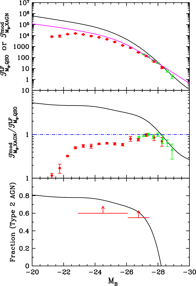
Figure 9.— Model (c) for the $B$-band. The upper panel represents the comparison of the time integral of the $B$-band QSO LF and that inferred from the local BHMF by adopting the reference model. The black line represents the value inferred from the local BHMF by using the reference model, i.e., model (c) with parameters $(\epsilon,\xi,\zeta)=(0.16,10,0.20)$ (similarly in middle and bottom panels). The magenta line represents the values obtained from the fitting-formula of the QSO LF obtained by Richards et al. (2005). The points have similar meanings as in Fig. 3. The middle panel shows the ratio of the values represented by the black line and the points in the upper panel to the values represented by the magenta line, i.e., the values in units of that inferred from the fitting-formula of the QSO LF. The bottom panel shows the fraction of optically obscured AGNs inferred from the reference model. The upper arrows show the lower limit of the fraction of optically obscured AGN at $z<0.3$ ($M_{\rm B}\sim-22.9$ —$-26.1$) and $0.3<z<0.83$ ($M_{\rm B}\sim-26.1$ —$-27.5$), respectively (Reyes et al., 2008), which are consistent with the prediction of the reference model in this paper. The range of $M_{\rm B}$ is converted from the luminosity range of [OIII] 5008Å line [using $\log(L[OIII]/L_{\sun})=-0.38M_{2400}-0.62$ in Fig. 11 in Reyes et al. (2008), where $M_{2400}$ is the absolute magnitude at 2400Å in the rest frame, and $M_{\rm B}\sim M_{2400}+0.13$ by assuming a canonical optical spectral slope ($\sim 0.5$) of QSOs].

6. The Eddington-ratio distribution in QSOs

Observational determination of the Eddington ratio distribution in QSOs can put additional constraints on MBH growth. These are independent of, but should be consistent with, the constraints obtained above from the extended Sołtan argument. Recent observational advances allow us to seriously estimate the Eddington ratio distribution in large samples of QSOs. For example, using the virial mass estimators Kollmeier et al. (2006) and Shen et al. (2007) have shown that the logarithm of Eddington-ratio distribution in high-luminosity QSOs resembles a Gaussian distribution with mean around $10^{-0.6}$ to $10^{-1.1}$ and width typically of 0.3 dex (see also Netzer et al. 2007), which may suggest that MBHs obtain most of their mass through accretion with a rate close to the Eddington limit. In this section, we check whether the luminosity evolution of individual QSOs constrained above is consistent with the observational Eddington ratio distribution.

In § 4, we have shown that the time-integrals of XAGN LF inferred from the local BHMF can be well matched to the observations using model (c) with parameters ($\epsilon$, $\xi$, $\zeta$)=(0.16, 10, 0.20) for the luminosity evolution of individual QSOs. In this reference model, the luminosity evolution and correspondingly the Eddington ratio evolution of a QSO are illustrated in Figure 10. As shown in the upper panel of Figure 10, the luminosity of a QSO exponentially increases to its peak luminosity with the Eddington rate set by the self-regulation of disk accretion when the fuel is over-supplied, and then decays with time as a power-law set by the self-similar evolution of disk accretion when the fuel is substantially under-supplied. The period for the QSO to have luminosity larger than $10\%$ of its peak luminosity is only a few times the Salpeter timescale. Correspondingly the Eddington ratio of the QSO is initially about $1$ and then also decays with time approximately as a power-law (the bottom panel of Fig. 10). The timescale for $\dot{m}$ declining from $1$ to $0.1$ is relatively short compared to the Salpeter timescale, and those QSOs around its peak luminosity should mainly accrete material via Eddington ratio close to $1$. As mentioned in § 1, the QSO LF at different redshifts involves the dependence on both the nuclear activity triggering rate ${\cal G}(z;M_{\bullet,0})$ and the luminosity evolution of individual QSOs ${\cal L}(\tau;M_{\bullet,0})$ after their nuclear activity being triggered, so does the QSO Eddington-ratio distribution at different redshifts. Below we define a ‘time-integrated’ Eddington-ratio distribution in QSOs, which only involves the accretion-rate evolution of individual QSOs.

Figure 10.— The luminosity and Eddington ratio (i.e., the accretion rate in units of the Eddington rate) evolution curves in the reference model, i.e., model (c) with parameters ($\epsilon$, $\xi$, $\zeta$)=($0.16$, $10$, $0.20$). In the initial rapid accretion phase, the luminosity of a QSO exponentially increases and the Eddington ratio is a constant ($\sim 1$) due to the self-regulation of the disk accretion when the accretion material is over-supplied, and both the luminosity and Eddington ratio of the QSO are followed by a rapid power-law-like decline due to the exhaustion of fuel and the self-similar evolution of disk accretion (see also Yu et al. 2005).

With a luminosity evolution model, the true Eddington ratio ($\dot{m}^{\rm r}$) distribution at a fixed bolometric luminosity $L_{\rm bol}$ for a MBH with present-day or final mass $M_{\bullet,0}$ is

$$P(\dot{m}^{\rm r}|L_{\rm bol},M_{\bullet,0})d\dot{m}^{\rm r}=\delta(\dot{m}^{\rm r}-\dot{m}_{0})d\dot{m}^{\rm r},$$ (45)

where $\dot{m}_{0}=1$ if the luminosity evolution is in the first rapidly increasing phase, $\dot{m}_{0}=M_{\bullet,\rm Edd}(L_{\rm bol})/M_{\bullet}^{\tau}$ if in the decline phase, and $M_{\bullet}^{\tau}$ is the mass of the MBH in a QSO with bolometric luminosity $L_{\rm bol}$ and with its final mass $M_{\bullet,0}$. The $M_{\bullet}^{\tau}$ can be directly obtained from equation (39) or (40) for fixed $L_{\rm bol}$ and $M_{\bullet,0}$. With given $P(\dot{m}^{\rm r}|L_{\rm bol},M_{\bullet,0})$, the (‘time-integrated’) probability distribution of the Eddington ratios among QSOs at a given $L_{\rm bol}$ can be defined by

$$P(\dot{m}^{\rm r}|L_{\rm bol})=\int n(M_{\bullet,0})\tau_{\rm lt}(M_{\bullet,0})\times$$

$$P(L_{\rm bol}|M_{\bullet,0})P(\dot{m}^{\rm r}|L_{\rm bol},M_{\bullet,0})dM_{\bullet,0}\times$$

$$\left[\int n(M_{\bullet,0})\tau_{\rm lt}(M_{\bullet,0})P(L_{\rm bol}|M_{\bullet,0})dM_{\bullet,0}\right]^{-1}$$ (46)

Note that the denominator in the above equation is just the time integral of the QSO LF.

Adopting the reference model for the luminosity evolution of individual QSOs, we calculate the probability distribution of underlying Eddington ratios among QSOs at a given $L_{\rm bol}$. As shown in Figure 11, the probability of finding objects with low Eddington ratios in low-luminosity QSOs is larger than that in high-luminosity QSOs. The average Eddington ratio in high-luminosity QSOs is larger than that in low-luminosity QSOs and the width of the Eddington-ratio distribution in high-luminosity QSOs is narrower than that in low luminosity QSOs, although the Eddington-ratio (or the accretion-rate) evolution in individual QSOs is assumed to be uniform. The $\delta$-function like distribution at $\dot{m}^{\rm r}=1$ [where we use $\frac{1}{a\sqrt{\pi}}\exp(-x^{2}/a^{2})$ with $a=0.1$ to mimic the Dirac function $\delta(\dot{m}^{\rm r}-1)$ for convenience] for each given $L_{\rm bol}$ represents the self-regulated rapid accretion phase with a rate close to the Eddington limit when the accretion material is over-supplied. Given an $L_{\rm bol}$, a lower Eddington ratio corresponds to a higher MBH mass, and the exponential decline of the probability distribution of Eddington ratios at small $\dot{m}^{\rm r}$ for QSOs at a given $L_{\rm bol}$ is primarily due to the exponential-like decay of MBH abundance at the high-mass end ($M_{\bullet}>10^{8}M_{\odot}$). The Eddington ratios in most of the luminous QSOs ($L_{\rm bol}\gtrsim 10^{45.75}\rm erg~{}s^{-1}$) are close to $1$ because of the steep falloff of the BHMF at the high-mass end and the rapid decay of Eddington ratios with time in the declining phase of the accretion-rate evolution in individual QSOs. These underlying Eddington-ratio distributions are clearly different from those observational estimates, i.e., a Gaussian distribution of $\dot{m}^{\rm obs}$ with peaks around $10^{-0.6}-10^{-1.1}$ (Kollmeier et al., 2006; Shen et al., 2007; Netzer et al., 2007).

The observationally estimated Eddington-ratio distribution may be biased from the underlying true Eddington ratio distribution. The reasons are: (1) the masses of MBHs in QSOs are usually obtained by using the virial mass estimator(s) $M_{\bullet}^{\rm vir}$, and the virial mass estimator is based on the analysis of broad emission line reverberation mapping data for several tens of low-luminosity AGNs at low redshift and a calibration of it to the local $M_{\bullet,0}-\sigma$ relation. The estimates of $M_{\bullet}^{\rm vir}$ may scatter around and be offset from the real $M_{\bullet}^{\rm r}$, as the relation between luminosity and broad line region (BLR) size and the relation between FWHM of emission lines and BLR virial velocity, adopted in the virial mass estimator(s), are not perfect, and its validation for high luminosity QSOs at high redshift is not fully tested (e.g., Kaspi et al., 2007). A scatter of $0.3$ dex in inferred $M_{\bullet}^{\rm vir}$ is plausible as pointed out by Kollmeier et al. (2006) (see also Shen et al. 2007) because the relation between observed line width and MBH mass may depend on the viewing angle of BLR (e.g., Krolik, 2001) and the relation between BLR size and luminosity has an intrinsic scatter about $0.1-0.2$ dex (Kaspi et al., 2005). (2) There may be some systematic errors as large as a factor of 3 or more either up or down in the virial mass estimator(s) due to various effects, such as, a broad radial emissivity distribution, and an unknown angular radiation pattern of line emission (see Krolik, 2001). These systematic errors may introduce an offset of the virial mass estimator(s) from the underlying true mass. (3) The bolometric luminosities are usually obtained using a uniform bolometric correction (see Kollmeier et al., 2006; Shen et al., 2007), but the real bolometric corrections may scatter around this uniform mean value by $\sim 0.1$ dex in the optical band (see § 3.3). The dominant bias is probably those introduced by the viral mass estimator(s).

We assume that the probability distribution of $M_{\bullet}^{\rm vir}$ for a given underlying real MBH mass $M_{\bullet}^{\rm r}$ is

$$P(\log M_{\bullet}^{\rm vir}|\log M_{\bullet}^{\rm r})=\frac{1}{\sqrt{2\pi}\Delta_{\log M_{\bullet}^{\rm vir}}}\times$$

$$\exp\left[-\frac{(\log M_{\bullet}^{\rm vir}-\log M_{\bullet}^{\rm r}-\Theta_{\log M_{\bullet}^{\rm vir}})^{2}}{2\Delta^{2}_{\log M_{\bullet}^{\rm vir}}}\right],$$ (47)

where $\Delta_{\log M_{\bullet}^{\rm vir}}$ is the scatter of MBH masses estimated by using the virial mass estimator(s) around the underlying given true mass, and $\Theta_{\log M_{\bullet}^{\rm vir}}$ is the offset of $\log M_{\bullet}^{\rm vir}$ from the true mass of MBHs $\log M_{\bullet}^{\rm r}$. As discussed above, it is plausible that $\Delta_{\log M_{\bullet}^{\rm vir}}\sim 0.3$ dex and $\left|\Theta_{\log M_{\bullet}^{\rm vir}}\right|\lesssim(0.3-0.6)$ (e.g., Krolik, 2001; Kollmeier et al., 2006; Shen et al., 2007). For a given $\dot{m}^{\rm r}$ at fixed $L_{\rm bol}$ and $M_{\bullet,0}$, the observationally estimated Eddington ratio is thus given by

$$P(\dot{m}^{\rm obs}|\dot{m}^{\rm r})=\frac{1}{\sqrt{2\pi}\ln(10)\Delta_{\log M_{\bullet}^{\rm vir}}\dot{m}^{\rm obs}}\times$$

$$\exp\left[-\frac{(\log\dot{m}^{\rm obs}-\log\dot{m}^{\rm r}+\Theta_{\log M_{\bullet}^{\rm vir}})^{2}}{2\Delta^{2}_{\log M_{\bullet}^{\rm vir}}}\right],$$ (48)

Combining this probability distribution with equation (46), the ‘time-integrated’ observational Eddington ratio ($\dot{m}^{\rm obs}$) distribution can be inferred from the local BHMF as

$$P(\dot{m}^{\rm obs}|L_{\rm bol})=\int d\dot{m}^{\rm r}P(\dot{m}^{\rm obs}|\dot{m}^{\rm r})\int n(M_{\bullet,0})\times$$

$$\tau_{\rm lt}(M_{\bullet,0})P(L_{\rm bol}|M_{\bullet,0})P(\dot{m}^{\rm r}|L_{\rm bol},M_{\bullet,0})dM_{\bullet,0}\times$$

$$\left[\int n(M_{\bullet,0})\tau_{\rm lt}(M_{\bullet,0})P(L_{\rm bol}|M_{\bullet,0})dM_{\bullet,0}\right]^{-1},$$ (49)

provided that the accretion rate or luminosity evolution of individual QSOs, i.e., ${\cal L}(\tau;M_{\bullet,0})$ and thus $P(L_{\rm bol}|M_{\bullet,0})$, is known.

We show $P(\dot{m}^{\rm obs}|L_{\rm bol})$ calculated from the reference model in Figure 12, using equation (49) and assuming $\Delta_{\log M_{\bullet}^{\rm vir}}=0.3$ dex and $\Theta_{\log M_{\bullet}^{\rm vir}}=0.6$ dex (for which the Eddington ratio in the first rapid accretion phase is $\dot{m}^{\rm r}=\dot{m}^{\rm r}_{P}=1$). It appears that the ‘time-integrated’ Eddington-ratio distribution is approximately a Gaussian distribution at any fixed bolometric luminosity $L_{\rm bol}\gtrsim 10^{45.75}\rm erg~{}s^{-1}$ but with a small tail at the low-Eddington ratio end. The Gaussian-like distribution mainly corresponds to the peaks at $\dot{m}^{\rm r}=1$ as shown in Figure 11, which represent the rapid accretion phase of individual QSOs with a rate self-regulated by the Eddington limit. The width of the Gaussian-like distribution mainly reflects the scatter $\Delta_{\log M_{\bullet}^{\rm vir}}$ in the estimates of MBH masses using the virial mass estimator(s), and the locations of peaks in the Eddington ratio distribution are roughly determined by the offset $\Theta_{\log M_{\bullet}^{\rm vir}}$ and the value of Eddington ratio $\dot{m}^{\rm r}_{P}$ during the self-regulated rapid accretion phase when the accretion material is over-supplied. For QSOs with lower bolometric luminosities ($L_{\rm bol}\lesssim 10^{45.25}\rm erg~{}s^{-1}$), the probability of finding low Eddington-ratio ($\dot{m}^{\rm obs}\lesssim 0.03$) objects becomes significant, which is primarily because the underlying MBH mass function is shallow at the low-mass end ($M_{\bullet}\lesssim 10^{8}M_{\odot}$) and the decline phase of the self-similar evolution of the disk accretion (see also Fig. 10) around big MBHs contributes significantly to the counts of low bolometric luminosity objects. Therefore, the Eddington ratio distribution among low-luminosity QSOs should provide independent constraints on the long-term evolution of disk accretion, especially in the decline phase (see also Yu et al. 2005).

Figure 11.— The underlying ‘time-integrated’ Eddington ratio distribution among QSOs at a given bolometric luminosity inferred from the reference model in § 4. From left to right at the low-Eddington ratio end, the lines represent $P(\dot{m}^{\rm r}|L_{\rm bol})$ at the given bolometric luminosity $L_{\rm bol}=10^{43.75}$ (solid line), $10^{44.25}$ (dotted line), $10^{44.75}$ (short-dashed line), $10^{45.25}$ (long-dashed line), $10^{45.75}$ (dot-short-dashed line), $10^{46.25}$ (dot-long-dashed line), $10^{46.75}$ (short-dash-long-dashed line), and $10^{47.25}\rm erg~{}s^{-1}$ (solid line), respectively. See details in § 6.

Except for giving a rough comparison with observations below, we do not intend to use $P(\dot{m}^{\rm obs}|L_{\rm bol})$ inferred from the reference model in this paper to directly fit the observational Eddington ratio distribution estimated by Kollmeier et al. (2006), Shen et al. (2007), and Netzer et al. (2007). The reasons are: (1) $P(\dot{m}^{\rm obs}|L_{\rm bol})$ obtained from equation (49) is a ‘time-integrated’ and volume-weighted Eddington-ratio distribution, while the current observationally estimated distributions are for given redshift intervals and not volume weighted. If the Eddington-ratio distribution at a given bolometric luminosity is independent of redshift as suggested by Kollmeier et al. (2006) (but perhaps it is not as argued by Shen et al. 2007), the ‘time-integrated’ Eddington ratio distribution among QSOs may represent the observational one for different redshift intervals; (2) the observational Eddington ratio distribution may be biased significantly at low Eddington ratios in flux-limited surveys, such as the SDSS (see Kollmeier et al. 2006 and Shen et al. 2007; for more general discussion of selection bias see also Lauer et al. 2007b and Yu & Lu 2004b); (3) $P(\dot{m}^{\rm obs}|L_{\rm bol})$ obtained from equation (49) does not distinguish obscured and unobscured QSOs, while the observationally estimated distribution is primarily obtained from optical QSO samples. If the obscuration is only a geometrical effect, then $P(\dot{m}^{\rm obs}|L_{\rm bol})$ may be the same as the Eddington-ratio distribution in optical QSO samples; however, if the obscuration is partly due to an evolutionary effect (e.g., QSOs may be more likely obscured in their early accretion stage), the probability of QSOs with high Eddington ratios may be suppressed.

If the MBH masses inferred from the virial mass estimator have an offset $\sim 0.5-0.6$ dex from the underlying true masses and also a scatter of $\sim 0.3$ dex around them, $P(\dot{m}^{\rm obs}|L_{\rm bol})$ at any fixed bolometric luminosities $L_{\rm bol}\gtrsim 10^{45.75}\rm erg~{}s^{-1}$ is roughly consistent with the Gaussian-like distribution of Eddington ratios (with a scatter of $\sim 0.3$ dex, and peak at $1/4$) among QSOs estimated by Kollmeier et al. (2006); however, $P(\dot{m}^{\rm obs}|L_{\rm bol})$ at bolometric luminosity $L_{\rm bol}\lesssim 10^{45.25}\rm erg~{}s^{-1}$ has a tail extended to lower Eddington ratios ($\dot{m}^{\rm obs}\lesssim 0.01$), which appears to conflict with that obtained by Kollmeier et al. (2006) for QSOs with $L_{\rm bol}<10^{45.5}\rm erg~{}s^{-1}$. The Eddington ratio in the self-regulated rapid accretion phase is assumed to be $1$ (i.e., exactly the Eddington limit) in the above calculations, but it may be slightly different from $1$ and a little smaller. For example, if $\dot{m}^{\rm r}=\dot{m}^{\rm r}_{P}=0.5$ in the first rapid accretion phase of the model (c), the time-integral of XAGN LF inferred from the local BHMF can still marginally match that obtained from observations, but it cannot if $\dot{m}^{\rm r}=\dot{m}^{\rm r}_{P}$ is substantially less than $0.5$. If $\dot{m}^{\rm r}_{P}=0.5$, to reproduce the observational Eddington ratio distribution at high bolometric luminosity ($L_{\rm bol}\gtrsim 10^{45.75}\rm erg~{}s^{-1}$), $\Theta\sim 0.2-0.3$ dex is required; and the tail of $P(\dot{m}^{\rm obs}|L_{\rm bol})$ at low Eddington ratios for low-luminosity QSOs ($L_{\rm bol}\lesssim 10^{45.25}\rm erg~{}s^{-1}$) is still significant, though less significant compared to the case for $\dot{m}^{\rm r}=\dot{m}^{\rm r}_{P}=1$ in the first rapid accretion phase.

The consistency between $P(\dot{m}^{\rm obs}|L_{\rm bol})$ inferred from the extended Sołtan argument and the observationally estimated Eddington-ratio distribution at high bolometric luminosity ($L_{\rm bol}\gtrsim 10^{45.75}\rm erg~{}s^{-1}$) suggests that the majority of bright QSOs accrete material at a single rate close to the Eddington limit. But we should be cautious of any over-interpretation of the possible inconsistency at low bolometric luminosity ($L_{\rm bol}\lesssim 10^{45.25}\rm erg~{}s^{-1}$) above, since the observational results obtained by different authors have not yet converged (e.g., Kollmeier et al., 2006; Shen et al., 2007; Netzer et al., 2007). For example, the observational Eddington-ratio distribution among QSOs with $L_{\rm bol}<10^{45.5}\rm erg~{}s^{-1}$ obtained by Shen et al. (2007) (i.e., a Gaussian-like distribution with peak at $10^{-1.1}$ and a scatter of $0.42$ dex) is substantially shifted to lower Eddington ratios compared with that obtained by Kollmeier et al. (2006) (i.e., a Gaussian-like distribution with peak $10^{-0.6}$ and scatter $0.3$ dex). Note also that the Eddington ratios in low-luminosity AGNs at low redshifts do cover a wide range as shown by Woo & Urry (2002), Heckman et al. (2004), and Greene & Ho (2007), which may be consistent with the prediction obtained from equation (49) above.

The offset $\Theta_{\log M_{\bullet}^{\rm vir}}\sim 0.3-0.6$ dex required by the above observational constraints suggests that the MBH masses inferred from the virial mass estimator(s) may be over-estimated by a factor of $2-4$, at least for high-luminosity QSOs, which is compatible with the possible systematic errors in the MBH mass estimated by the reverberation mapping technique (Krolik, 2001). If this offset is real, it is intriguing and important since many current studies on the growth and evolution of MBHs in QSOs are based on the virial mass estimator(s). For example, the masses of MBHs in two samples of AGNs at redshifts $z=0.36$ and $z=0.57$, estimated from the virial mass estimator(s), are found to be larger than that estimated from the local $M_{\bullet,0}-\sigma$ relation by $0.54$ dex and $0.51$ dex, respectively (Treu et al., 2004; Woo et al., 2006, 2008), which is suggested as an indicator of that the growth of MBHs predates the final growth of bulges in these AGN host galaxies. If MBH masses from the virial mass estimator(s) are generally over-estimated by a factor of $2-4$ as argued above, then there should be not much difference between the rescaled virial masses and that predicted from the $M_{\bullet}-\sigma$ relation for those MBHs in the studies of Treu et al. (2004) and Woo et al. (2006, 2008).

Similar to the probability distribution of the Eddington ratio among QSOs at a given bolometric luminosity given in equation (46), the probability distribution of the Eddington ratio among QSOs at a given MBH mass $M_{\bullet}^{\rm r}$ can be estimated by

$$P(\dot{m}^{\rm obs}|M_{\bullet}^{\rm r})=\int d\dot{m}^{\rm r}P(\dot{m}^{\rm obs}|\dot{m}^{\rm r})\int n(M_{\bullet,0})\times$$

$$\tau_{\rm lt}(M_{\bullet,0})P(M_{\bullet}^{\rm r}|M_{\bullet,0})P(\dot{m}^{\rm r}|M_{\bullet}^{\rm r},M_{\bullet,0})dM_{\bullet,0}\times$$

$$\left[\int n(M_{\bullet,0})\tau_{\rm lt}(M_{\bullet,0})P(M_{\bullet}^{\rm r}|M_{\bullet,0})dM_{\bullet,0}\right]^{-1},$$ (50)

or the probability distribution of Eddington ratio among QSOs at a given $M_{\bullet}^{\rm vir}$ can be estimated as

$$P(\dot{m}^{\rm obs}|M_{\bullet}^{\rm vir})=\int d\dot{m}^{\rm r}P(\dot{m}^{\rm obs}|\dot{m}^{\rm r})\int dM_{\bullet}^{\rm r}P(M_{\bullet}^{\rm vir}|M_{\bullet}^{\rm r})\times$$

$$\int n(M_{\bullet,0})\tau_{\rm lt}(M_{\bullet,0})P(M_{\bullet}^{\rm r}|M_{\bullet,0})P(\dot{m}^{\rm r}|M_{\bullet}^{\rm r},M_{\bullet,0})dM_{\bullet,0}/$$

$$\int P(M_{\bullet}^{\rm vir}|M_{\bullet}^{\rm r})dM_{\bullet}^{\rm r}\int n(M_{\bullet,0})\tau_{\rm lt}(M_{\bullet,0})P(M_{\bullet}^{\rm r}|M_{\bullet,0})dM_{\bullet,0},$$

(51)

where $P(M_{\bullet}^{\rm vir}|M_{\bullet}^{\rm r})=P(\log M_{\bullet}^{\rm vir}|\log M_{\bullet}^{\rm r})/[M_{\bullet}^{\rm vir}\ln(10)]$. We note here that $P(\dot{m}^{\rm obs}|M_{\bullet}^{\rm vir})$ should be skewed toward low Eddington ratios because a QSO may spend a majority of its lifetime in the declining phase with small $\dot{m}^{\rm r}$ ($<0.1$) as that revealed by the reference model in this paper (e.g., Fig 10). However, it is not easy to observationally estimate $P(\dot{m}^{\rm obs}|M_{\bullet}^{\rm vir})$ since low-luminosity QSOs are more likely to be missed in flux-limited surveys, especially at high redshift (see also discussions in Kollmeier et al., 2006). We defer the comparison of this distribution with observations to future work.

Figure 12.— The observational ‘time-integrated’ Eddington ratio distribution among QSOs at a given bolometric luminosity inferred from the reference model in § 4 by assuming that the scatter and offset in the masses of MBHs obtained from the virial mass estimator(s) are $0.3$ dex and $0.6$ dex, respectively. The line types have the same meaning as in Fig. 11.

7. Toy models for mergers

7.1. Gas-poor (dry) mergers

In current hierarchical galaxy formation models, mergers of galaxies are the main route to form elliptical galaxies and stellar bulges (e.g., Kauffmann, White & Guiderdoni, 1993; Cole et al., 2000). If each merging galaxy has a central MBH, mergers of two galaxies will inevitably form binary MBHs and may further lead to mergers of MBHs if their inspiral and orbital evolution time is shorter than a Hubble time (e.g., Begelman, Blandford & Rees, 1980; Yu, 2002). Mergers of MBHs occurred after the quenching of nuclear activity, as the probable consequence of galaxy gas-poor (dry) mergers, may significantly re-shape the BHMF established by accretion processes. Below we use a toy model to illustrate the change of the BHMF due to BH mergers under the assumption that MBHs grow only by merging BHs but with little accretion directly onto MBHs during the galaxy dry merger stage.

Assume that a major dry merger of two host galaxies always leads to the merger of their central MBHs with mass ratio of $\alpha=M_{\bullet,2}/(M_{\bullet,1}+M_{\bullet,2})$ (e.g., 0.5 or 0.25 for a 1:1 or 1:3 merger) after the nuclear activity is quenched, where $M_{\bullet,1}$ and $M_{\bullet,2}$ are the masses of the two BHs before their merger. The merged BH mass is $M_{\bullet,0}=\beta(M_{\bullet,1}+M_{\bullet,2})$ and ($1-\beta$) is the fraction of energy (or mass) losses due to gravitational waves during the MBH merger process. Thus, the mass function of QSO remnants right after the nuclear activity is

$$n^{\prime}_{M_{\bullet}}(M_{\bullet,0}^{\prime}) = \int dM_{\bullet,0}n_{M_{\bullet}}(M_{\bullet,0})\times$$ (52)

$$\left[\delta(M_{\bullet,0}^{\prime}-\frac{\alpha}{\beta}M_{\bullet,0})+\delta(M_{\bullet,0}^{\prime}-\frac{1-\alpha}{\beta}M_{\bullet,0})\right]$$

$$= \frac{\beta}{\alpha}n_{M_{\bullet}}(M_{\bullet,0})|_{M_{\bullet,0}=\frac{\beta}{\alpha}M_{\bullet,0}^{\prime}}+$$

$$\frac{\beta}{1-\alpha}n_{M_{\bullet}}(M_{\bullet,0})|_{M_{\bullet,0}=\frac{\beta}{1-\alpha}M_{\bullet,0}^{\prime}}.$$

Note this mass function $n^{\prime}_{M_{\bullet}}(M_{\bullet,0}^{\prime})$ is non-synchronous since the last major (dry) merger may occur at different time for different MBHs.

During the merging process of BHs (which is divided into three phases: inspiral, merger and ringdown), the total energy lost through gravitational waves, $E_{\rm rad}$ is difficult to calculate, especially for the merger of two BHs with large spins, but roughly in the range $0.03M_{\bullet,12}F(\mu/M_{\bullet,12})<E_{\rm rad}<0.2M_{\bullet,12}F(\mu/M_{\bullet,12})$, where $M_{\bullet,12}=M_{\bullet,1}+M_{\bullet,2}$ is the total (initial) mass of the two BHs, $\mu$ is the reduced mass and $F(\mu/M_{\bullet,12})=(4\mu/M_{\bullet,12})^{2}$ (see eq. 3.7 in Flanagan & Hughes, 1998). Recent breakthrough in relativistic numerical calculation of merging binary BHs due to Pretorius (2005) and Baker et al. (2006) has shown that on the order of 5% of the initial rest mass for a system of two equal mass, nonspinning BHs is radiated as gravitational waves during the final orbit and ringdown, which is consistent with the estimate in Flanagan & Hughes (1998). For the merging of equal mass, rapidly spinning BHs, the energy radiated as gravitational wave could be larger and the upper limit is about 24% if the final spin is around $0.9$ (e.g., Pretorius & Khurana, 2007). Since the spin of MBHs is probably close to $0.7-0.9$ due to accretion processes (e.g., Gammie et al., 2004; Shapiro, 2005; Hawley et al., 2007), here we choose two cases, 10% and 24% of the initial total rest mass, for the amount of energy radiated as gravitational waves, and therefore $\beta=1-0.1F(\mu/M_{\bullet,12})$ and $1-0.24F(\mu/M_{\bullet,12})$, respectively.

Using the data from Galaxy Evolution from Morphology and SEDs (GEMS), Bell et al. (2006) find that present-day spheroidal galaxies with $M_{V}<-20.5$ on average have undergone between 0.5 and 2 major dry mergers since redshift $z<0.7$ (see also similar results in Conselice et al. 2003 for redshift $z\lesssim 3$, and Lin et al. 2004 for redshift $z\lesssim 1.2$). MBHs with mass substantially less than $10^{8}M_{\odot}$ are mostly hosted by the stellar bulges of spiral galaxies, which should not have undergone a significant number of major dry mergers in the near past (e.g., $z\lesssim 1$) since their disks are preserved. For simplicity, here we assume all MBHs with $M_{\bullet,0}\gtrsim 10^{8}M_{\odot}$, corresponding to $M_{V}<-20.5$, have experienced one major dry merger after the quenching of nuclear activity, while smaller MBHs did not experience major dry mergers. Using equation (52) to correct the effect due to dry mergers in $n_{M_{\bullet}}(M_{\bullet,0})$, the BHMF right after the quenching of nuclear activities, $n_{M_{\bullet}}(M_{\bullet,0}^{\prime})$, which is established by the accretion process, is estimated and shown in Figure 13. As seen from Figure 13, the abundance of MBHs with mass larger than a few $10^{9}M_{\odot}$ may be enhanced at most by a factor $\sim 2-3$ due to the major dry mergers after the quenching of nuclear activities. This enhancement is not so prominent compared with that in the estimate of BHMF due to the uncertainty in the intrinsic scatters in the $M_{\bullet,0}-\sigma$ and $M_{\bullet,0}-L_{\rm bulge}$ relationships. For example, a slight error in the estimated intrinsic scatters, e.g., $0.05$ dex, could introduce an uncertainty larger than a factor of $\sim 2-3$ at the high-mass end of the BHMF. Therefore, we conclude that it is safe to neglect the uncertainty in the BHMF due to major dry mergers after the quenching of nuclear activities in our calculations as the intrinsic scatters in the $M_{\bullet,0}-\sigma$ or $M_{\bullet,0}-L_{\rm bulge}$ relations are currently not well determined.

Figure 13.— Effect of dry mergers on re-shaping the BHMF after the quenching of nuclear activity. The solid line represent the BHMF $M_{\bullet,0}n_{M_{\bullet}}(M_{\bullet,0})$ in the local universe estimated by the $M_{\bullet,0}-\sigma$ relation and the velocity-dispersion distribution as that shown in Fig. 1. The dashed and dotted lines show the BHMF $n_{M_{\bullet}}(M_{\bullet}^{\prime})$ after correcting the effect due to dry mergers. Dotted (or dashed) lines represent the case that all MBHs with mass $>10^{8}M_{\odot}$ experienced one 1:1 (or 1:3) dry major merger, while other MBHs with smaller mass have not undergone any major mergers, after the quenching of nuclear activity. The loss of energy through gravitational waves are assumed to be 10% (thick dotted or dashed lines) or 24% (thin dotted or dashed lines) of the initial total rest mass. This figure shows that the abundance of MBHs after the quenching of nuclear activity may be smaller than that estimated in the local universe at most by a factor of 2–3 at the high-mass end, but is not significantly different from the local BHMF at the low-mass end. This difference caused by the effect of dry mergers on the estimated BHMF is not so prominent compared with that due to the uncertainty of intrinsic scatters in the $M_{\bullet,0}-\sigma$ and $M_{\bullet,0}-L_{\rm bulge}$ relations.

7.2. Gas-rich (wet) mergers

For a present-day MBH with mass $M_{\bullet,0}$, its host galaxy may have undergone more than one (wet) major merger. By ‘wet’ major merger here we mean gas-rich major mergers (spiral+spiral or spiral+elliptical) which lead to substantial gas fueling to trigger nuclear activity. In the current scenario of hierarchical formation and co-evolution of galaxies and MBHs (e.g., Kauffmann & Haehnelt, 2000; Bower et al., 2006; Croton et al., 2006; Malbon et al., 2007), each ‘wet’ major merger leads to a nuclear active phase with substantial increase in the central MBH mass. For a local MBH we see today, it may build up through multiple times of nuclear activity and mergers of smaller MBHs, and thus our assumption of a single time of nuclear activity in § 4 may be an over-simplification. In order to estimate the effects of possible multiple phases of nuclear activity in the assembly history of a MBH, we assume that all MBHs experienced two or more ‘wet’ major mergers and its mass increases by a factor of $5$, $10$ or more after each ‘wet’ major merger, and this assumption is compatible with the current co-evolution models (e.g. Kauffmann & Haehnelt, 2000; Bower et al., 2006; Croton et al., 2006; Malbon et al., 2007). Before each ‘wet’ major merger, we assume that the MBH triggered by the ‘wet’ merger later is the merger remnant of two progenitors with mass ratio either $1:1$ or $1:3$. These two progenitors also experienced a similar period of significant mass growth before and so on and so forth. We can use this procedure backwards for two or more times to mimic multiple phases of accretion (including mergers). With the above assumptions, combining equations (52) and (24), the time-integral of XAGN LF can be calculated. In these calculations we also adopt the same parameters ($\epsilon$, $\zeta$, $\gamma$) as in the reference model but adjust $\xi$ in order to satisfy the assumption of a factor of $5$, $10$ or more mass increase during each ‘wet’ major merger. We find that the inferred value of the time-integral of XAGN LF at the low-luminosity end for the multiple-times nuclear activity assumption is larger than that obtained by assuming a single-time nuclear activity at most by $\sim 20-30\%$, and the difference is negligible at the high-luminosity end. We therefore conclude that the assumption of a single-time nuclear activity is good enough, provided that the masses of MBHs substantially increase (say, by a factor of $5$, $10$ or more) during the nuclear activity.

8. Further Implications

8.1. BHMF at redshift $z$

If the probability function $P(L|M_{\bullet,0})$ is known (for example, as described by the reference model we obtained from the extended Sołtan argument above), the BHMF at redshift $z$, i.e., $n_{M_{\bullet}}(M_{\bullet,0},t_{z})$ can be estimated by an equation similar to equation (1)

$$\int^{\infty}_{z}\Psi_{L}(L,z)\left|\frac{dt}{dz}\right|dz = \int^{\infty}_{0}n_{M_{\bullet}}(M_{\bullet,0},t_{z})\tau_{\rm lt}(M_{\bullet,0})\times$$ (53)

$$P(L|M_{\bullet,0})dM_{\bullet,0},$$

where $t_{z}=\int^{\infty}_{z}\left|\frac{dt}{dz}\right|dz$ is the cosmic time at redshift $z$. Equation (53) is true only if the BHMF at $z$ is dominated by quiescent MBHs.

If MBHs with final mass $M_{\bullet,0}$ shined for a time $\tau_{\rm lt}(M_{\bullet,0})$ with luminosity $L=\lambda L_{\rm Edd}(M_{\bullet})$ and without increasing their mass significantly ($M_{\bullet,0}\simeq M_{\bullet}$), where $\lambda$ is a constant and $L_{\rm Edd}(M_{\bullet})$ is the Eddington luminosity (see definition in eq. 25), then $P(L|M_{\bullet,0})\simeq\delta[L-\lambda L_{\rm Edd}(M_{\bullet,0})]$ and thus

$$n_{M_{\bullet}}(M_{\bullet,0},t_{0}) \simeq \frac{1}{\tau_{\rm lt}(M_{\bullet,0})}\int^{\infty}_{0}\Psi_{L}(L,z)|_{L=\lambda L_{\rm Edd}(M_{\bullet,0})}\times$$ (54)

$$\left|\frac{dt}{dz}\right|dz\times\lambda\left|\frac{dL_{\rm Edd}(M_{\bullet})}{dM_{\bullet}}\right|_{M_{\bullet}=M_{\bullet,0}}.$$

If these assumptions are correct, it appears that the local BHMF can be forced to be always consistent with the QSO LF by adjusting $\tau_{\rm lt}(M_{\bullet,0})$ and $\lambda$. Similarly, the BHMF at redshift $z$ is given by

$$n_{M_{\bullet}}(M_{\bullet,0},t_{z}) \simeq \frac{1}{\tau_{\rm lt}(M_{\bullet,0})}\int^{\infty}_{z}\Psi_{L}(L,z)|_{L=\lambda L_{\rm Edd}(M_{\bullet,0})}\times$$ (55)

$$\left|\frac{dt}{dz^{\prime}}\right|dz^{\prime}\times\lambda\left|\frac{dL_{\rm Edd}(M_{\bullet})}{dM_{\bullet}}\right|_{M_{\bullet}=M_{\bullet,0}}.$$

The BHMF at redshift $z$, $n_{M_{\bullet}}(M_{\bullet,0},t_{z})$, estimated from equation (55) may be not accurate if the real $\tau_{\rm lt}(M_{\bullet,0})$ is substantially longer than the Salpeter timescale since in this case the MBH mass was evolving rapidly during its active phase and the BHMF sharply decreases at the high-mass end, and also the assumption of $P\simeq\delta(L-\lambda L_{\rm Edd})$ is not good. The errors in the BHMF at redshift $z$ obtained from this simple approach can be estimated by comparing it with that obtained from equation (53). With the constraints on the luminosity evolution of individual QSOs obtained above, we will estimate the BHMF at different redshift $z$ and check whether these estimates are consistent with observations in a future study.

8.2. Triggering rate of nuclear activity

The QSO LF at redshift $z$ can be inferred as

$$\Psi_{L}(L,z) = \int dM_{\bullet,0}\int^{\infty}_{z}{\cal G}(z_{i};M_{\bullet,0})\delta(L-{\cal L}(\tau;M_{\bullet,0}))\times$$ (56)

$$\left|\frac{dt}{dz_{i}}\right|dz_{i}$$

where $\tau=t_{z}-t_{z_{i}}$. Given $\Psi_{L}(L,z)$ and ${\cal L}(\tau;M_{\bullet,0})$, the triggering rate of nuclear activity in the mass range $M_{\bullet,0}-M_{\bullet,0}+dM_{\bullet,0}$, ${\cal G}(z;M_{\bullet,0})$, can be solved from the above integral equation. Estimation of ${\cal G}(z;M_{\bullet,0})$ is of fundamental importance because it is this function that dominates the cosmic evolution of the QSO population and the down-sizing nature of the formation of MBHs. Here the cosmic evolution of the QSO population means that the comoving number density of the QSO population brighter than a certain luminosity (or in a certain luminosity range) has a peak at an intermediate redshift (e.g., $z\sim 2-3$) and decreases at both higher and lower redshift (e.g., Richards et al., 2006a; Hasinger et al., 2005) and the down-sizing nature refers to that observationally the characteristic mass of MBHs in QSOs decreases with decreasing redshifts (e.g., Marconi et al., 2004; Merloni, 2004). Given ${\cal G}(z;M_{\bullet,0})$ and ${\cal L}(\tau;M_{\bullet,0})$, many statistical properties of QSOs (for instance, the Eddington rate ratio distribution and the MBH mass distribution at different redshifts in QSOs/AGNs) can be inferred. Comparison of these inferred properties with those directly obtained from observations will further reveal details of the growth and evolution of MBHs and QSOs. We will present this in a future study.

9. Conclusions

In this paper, we have studied the observational constraints on the growth of MBHs using the extended Sołtan argument. In this approach, the local BHMF is directly connected with the time-integral of the QSO LF through only the luminosity evolution of individual QSOs (and correspondingly the accretion-rate evolution, given the mass-to-energy conversion efficiency), and the luminosity evolution of individual QSOs is isolated from the cosmic evolution of the triggering rate of nuclear activity. The luminosity (or accretion-rate) evolution of individual QSOs has an unambiguous physical definition, and it is different from the ‘mean accretion rate’ as a function of mass and/or redshift widely used in the literature (e.g., Marconi et al., 2004; Shankar et al., 2004, 2007) in that the ‘mean accretion rate’ is a combined property depending on both the luminosity evolution of individual QSOs and the cosmic evolution of the triggering rate of nuclear activity.

With recent knowledge of the relationships between MBH mass and host galaxy properties (either the $M_{\bullet,0}-\sigma$ relation or the $M_{\bullet,0}-L_{\rm bulge}$ relation) and the distribution of galaxy properties (either $\sigma$ or $L_{\rm bulge}$), we estimate the local BHMF. We obtain the time-integral of the QSO LF from recent estimates of QSO LFs in both optical and X-ray bands. Using the local BHMF and the time-integral of the QSO LF, we obtain robust constraints on the luminosity (or accretion rate) evolution of individual QSOs and important characteristic parameters describing the growth of individual MBHs, such as the mass-to-energy conversion efficiency and lifetime, which are summarized below.

• The luminosity (or accretion rate) evolution of individual QSOs probably involves two phases: an initially exponentially increasing phase set by the Eddington limit (i.e., ${\cal L}\simeq L_{\rm Edd}$) when the infall material to feed the central MBHs is over-supplied; and then followed by a phase with power-law declining set by a self-similar long-term evolution of disk accretion (i.e., ${\cal L}\propto\tau^{-\gamma}$ and $\gamma\sim 1.2-1.3$). With this type of luminosity evolution, the time-integral of QSO LF can be well matched by that inferred from the local BHMF. Other simple luminosity evolution models, such as a single Eddington ratio for all MBHs/QSOs or an initially exponentially increasing phase followed by an exponentially decay phase, cannot satisfy the extended Sołtan argument simultaneously at both the high-luminosity end and low-luminosity ends, and thus are ruled out.

• The mass-to-energy conversion efficiency $\epsilon$ is $\simeq 0.16\pm 0.04^{+0.05}_{-0}$ (correspondingly the spin parameter $a$ is in the range from $0.8$ to $0.99$) if adopting the local BHMF estimated from the $M_{\bullet,0}-\sigma$ relation, which is fully consistent with the theoretical expectations of $\sim 0.10-0.20$, i.e., the spin of MBHs in QSOs may stay at an equilibrium of $\sim 0.7-0.9$ for most of the QSO lifetime (e.g., Gammie et al., 2004; Shapiro, 2005; Hawley et al., 2007). However, the efficiency $\epsilon$ is reduced to $\simeq 0.08\pm 0.02^{+0.03}_{-0}$ (and correspondingly the spin parameter $a$ is in the range from $0.1$ to $0.8$) if adopting the local BHMF estimated from the $M_{\bullet,0}-L_{\rm bulge}$ relation, which is lower than but may be still marginally consistent with theoretical expectations.

• The lifetime of QSOs/AGNs, which depends on detailed definition of the nuclear activity or the lower threshold set to the active nuclear luminosity, can be as long as a few $10^{9}$ yr, and the characteristic timescale in the luminosity increasing phase and transition timescale to the declining phase do not necessarily depend on the mass of their central MBHs. The period that a QSO or MBH radiating at a luminosity larger than $10\%$ of its peak luminosity is only about $2-3\times 10^{8}$ yr, and during this period the MBH obtained most of its mass. If adopting the local BHMF estimated from the $M_{\bullet,0}-L_{\rm bulge}$ relation, the above values related to the QSO lifetime decrease by a factor $\sim 2$.

• For individual QSOs, the characteristic timescale for the luminosity (or accretion rate) to decline from its peak $L_{P}$ to $0.1L_{P}$ in their second phase should be relatively short compared to the Salpeter timescale, which suggests that the material infalling from a large galactic scale and deposited in the vicinity of MBHs be consumed by rapid accretion onto the central MBH and at the mean time further deposit of material can be efficiently suppressed by some mechanisms, probably the AGN feedback mechanism (e.g., Silk & Rees, 1998; King, 2003; Murray et al., 2005; Di Matteo et al., 2005), on a timescale $\lesssim\tau_{\rm S}$.

• The majority of high-luminosity ($L_{\rm bol}\gtrsim 10^{45.75}\rm erg~{}s^{-1}$) QSOs accrete material via an almost single Eddington ratio, close to 1 and not smaller than half of the Eddington limit, which suggests that the disk accretion onto MBHs should be indeed self-regulated by the Eddington limit when the accretion material is over-supplied in the initial phase.

• Low-luminosity QSOs ($L_{\rm bol}\lesssim 10^{45.25}\rm erg~{}s^{-1}$) accrete material via a much wider range of Eddington ratios, and a significant fraction of them accrete material via low Eddington ratio ($\dot{m}\lesssim 0.1$), which corresponds to the self-similar long-term evolution of disk accretion around MBHs ($M_{\bullet}\sim\tau^{-\gamma}$ and $\gamma\sim 1.2-1.3$) when the accretion material is under-supplied.

• The Eddington ratio distribution among QSOs/AGNs inferred from the extended Sołtan argument concentrates toward high Eddington ratios (close to 1), especially for high luminosity QSOs, which appears to conflict with that estimated directly from observations (with a mean value of $\sim 10^{-0.6}-10^{-1.1}$) by using the virial mass estimator(s). To make these two distributions consistent with each other, an offset of $0.3-0.6$ dex in the MBH mass estimated from the virial mass estimator(s) is required, at least for high-luminosity QSOs, which suggests that MBHs masses obtained from the virial mass estimator(s), have been systematically over-estimated by a factor of $2-4$.

• The fraction of optically obscured QSOs/AGNs inferred from the extended Sołtan argument can be as high as $80\%$ at $M_{\rm B}\sim-20$—$-23$ and slightly decreases to $60\%$ at $M_{\rm B}=-24$—$-27$, and these numbers are consistent with recent observations by Reyes et al. (2008). The dependence of the fraction of type 2 AGNs on the X-ray luminosity cannot be solely an evolutionary effect arising from their individual evolution after nuclear activity is triggered (i.e., QSOs are more likely to be obscured in the early stage of the MBH growth), and some other effects (e.g., those introduced by the receding torus model; Lawrence 1991) should be responsible for the larger fraction of type 2 AGNs at low luminosities ($L_{X}\lesssim 10^{43.5}\rm erg~{}s^{-1}$).

We estimate possible effects due to MBH mergers (which may re-shape the local BHMF) and multiple times of nuclear activity and accretion (e.g., triggered by multiple times of galaxy ‘wet’ major mergers) in the growth history of a MBH, and we find that these effects on our conclusions are insignificant, which again supports that the constraints obtained above are robust.

The constraints on the luminosity evolution of individual QSOs obtained from the extended Sołtan argument in this paper, together with the QSO LF, can be further used to derive the BHMF at high redshifts and the cosmic evolution of the triggering rate of nuclear activity. These constraints and those recent estimates on the Eddington ratio distribution in QSOs ask for serious theoretical modeling of the long-term evolution of disk accretion around MBHs. More detailed modeling of accretion and radiation transfer physics in the vicinity of MBHs may have to be involved to determine the self-regulation of the disk accretion (rather than the simple Eddington limit argument) at the initial phase with sufficient deposited accretion material. It should be one of the important long-term goals for theoretical studies on the growth of MBHs to answer questions like what determines the transition from the initial rapid accretion phase with Eddington ratio close to 1 to the rapid declining phase, what shuts off the efficient accretion process around MBHs (probably jointly determined by an efficient feedback mechanism and the accretion disk viscosity), and what determines the evolution of the spin of MBHs.

References

- Akylas et al. (2006) Akylas, A., Georgantopoulous, I., Georgakakis, A., Kitsionas, S., & Hatziminaglou, E. 2006, A&A, 459, 693
- Alexander et al. (2005) Alexander, D. M., Small, I., Bauer, F. E., Chapman, S. C., Blain, A. W., Brandt, W. N., & Ivison, R. J. 2005, Nature, 434, 738
- Aller & Richstone (2002) Aller, M. C., & Richstone, D. 2002, AJ, 124, 3035
- Aller & Richstone (2007) Aller, M. C., & Richstone, D. 2007, ApJ, 665, 120
- Armitage & Natarajan (2002) Armitage, P. J., & Natarajan, P. 2002, ApJ, 567, L9
- Baes et al. (2003) Baes, M., Buyle, P., Hau, G.K.T., & Dejonghe, H. 2003, MNRAS, 341, L44
- Baker et al. (2006) Baker, J. G., Centrella, J., Choi, D., Koppitz, M., & van Meter, J. 2006, PRL, 96, 1102
- Barger et al. (2005) Barger, A. J., Cowie, L. L., Mushotzky, R. F., Yang, Y., Wang, W.-H., Steffen, A. T., & Capak, P. 2005, AJ, 129, 578
- Batcheldor et al. (2007) Batcheldor, D., Marconi, A., Merritt, D., & Axon, D. J. 2007, ApJ, 663, L85
- Beckmann et al. (2006) Beckmann, V., et al. 2006, ApJ, 652, 126
- Begelman, Blandford & Rees (1980) Begelman, M. C., Blandford, R. D., & Rees, M. J. 1980, Nature, 287, 307
- Bell et al. (2006) Bell, E. F., et al. 2006, ApJ, 640, 241
- Bernardi et al. (2003) Bernardi, M., et al. 2003, AJ, 125, 1849
- Bernardi et al. (2006) Bernardi, M., Sheth, R. K., Nichol, R. C., Miller, C. J., Schlegel, D., Frieman, J., Schneider, D. P., Subbarao, M., York, D. G., & Brinkmann, J. 2006, AJ, 131, 2018
- Bernardi et al. (2007) Bernardi, M., Sheth, R. K., Tundo, E., & Hyde, J. B. 2007, ApJ, 660, 267
- Binney & Tremaine (2008) Binney, J., & Tremaine, S. 2008, Galactic Dynamics, 2nd Edition (Princeton: Princeton Univ. Press)
- Blandford (2003) Blandford, R. D. 2003, Carnegie Observatories Astrophysics Series, Vol. 1: Coevolution of Black Holes and Galaxies, ed. L. C. Ho (Cambridge: Cambridge Univ. Press)
- Blandford & Begelman (1999) Blandford, R. D., & Begelman, M. C. 1999, MNRAS, 303, L1
- Blanton et al. (2003) Blanton, M., et al. 2003, ApJ, 592, 812
- Bower et al. (2006) Bower, R. G., Benson, A. J., Malbon, R., Helly, J. C., Frenk, C. S., Baugh, C. M., Cole, S., & Lacey, C. G. 2006, MNRAS, 370, 645
- Boyle et al. (2000) Boyle, B. J., Shanks, T., Croom, S. M., Smith, R. J., Miller, L., Loaring, N., & Heymans, C. 2000, MNRAS, 317, 1014
- Caditz & Petrosian (1990) Caditz, D., & Petrosian, V. 1990, ApJ, 357, 326
- Cannizzo et al. (1990) Cannizzo, J. K., Lee, H. M., & Goodman, J. 1990, ApJ, 351, 38
- Cavaliere et al. (1971) Cavaliere, A., Morrison, P., & Wood, K. 1971, ApJ, 170, 223
- Cavaliere & Padovani (1989) Cavaliere, A., Padovani, P. 1989, ApJ, 340, L5
- Chokshi & Turner (1992) Chokshi, A., & Turner, E. L. 1992, MNRAS, 259, 421
- Ciotti & Ostriker (2007) Ciotti, L., & Ostriker, J. P. 2007, ApJ, 665, 1038
- Cole et al. (2000) Cole, S., Lacey, C. G., Baugh, C., & Frenk, C. S. 2000, MNRAS, 319, 168
- Comastri et al. (1995) Comastri, A., Setti, G., Zamorani, G., & Hasinger, G. 1995, A&A, 296, 1
- Conselice et al. (2003) Conselice, C. J., Bershady, M. A., & Dickinson, M. 2003, AJ, 126, 1183
- Croom et al. (2004) Croom, S. M., Smith, R. J., Boyle, B. J., Shanks, T., Miller, L., Outram, P. J., & Loaring, N. S. 2004, MNRAS, 349, 1397
- Croton et al. (2006) Croton, D. J., Springel, V., White, S. D. M., De Lucia, G., Frenk, C. S., Gao, L., Jenkins, A., Kauffmann, G., Navarro, J. F., Yoshida, N. 2006, MNRAS, 365, 11
- Di Matteo et al. (2005) Di Matteo, T., Springel, V., & Hernquist, L. 2005, Nature, 433, 604
- Efstathiou & Rees (1988) Efstathiou, G., & Rees, M. J. 1988, MNRAS, 230, 5P
- Elvis et al. (1994) Elvis, M., Wilkes, B. J., McDowell, J. C., Green, R. F., Bechtold, J., Willner, S. P., Oey, M. S., Polomski, E., & Cutri, R. 1994, ApJS, 95, 1
- Elvis et al. (2002) Elvis, M., Risaliti, G., & Zamorani, G. 2002, ApJ, 565, L75
- Escala et al. (2004) Escala, A., Larson, R. B., Coppi, P. S., & Mardones, D. 2004, ApJ, 607, 765
- Escala et al. (2005) Escala, A., Larson, R. B., Coppi, P. S., & Mardones, D. 2005, ApJ, 630, 152
- Fabian & Iwasawa (1999) Fabian, A. C., & Iwasawa, K. 1999, MNRAS, 303, 34
- Fan et al. (2001) Fan, X., et al. 2001, AJ, 121, 54
- Fan et al. (2003) Fan, X., et al. 2003, AJ, 125, 1649
- Ferrarese (2002) Ferrarese, L. 2002, ApJ, 578, 90
- Ferrarese & Ford (2005) Ferrarese, L., & Ford, H. 2005, Space Science Reviews, Volume 116, Issue 3-4, p523
- Ferrarese & Merritt (2000) Ferrarese, L., & Merritt, D. 2000, ApJ, 539, L9
- Flanagan & Hughes (1998) Flanagan, . ., & Hughes, S. A. 1998, Phys. Rev. D., 57, 05562821
- Fontanot et al. (2007) Fontanot, F., Cristiani, S., Monaco, P., Nonino, M., Vanzella, E., Brandt, W. N., Grazian, A., & Mao, J. 2007, A&A, 461, 39
- Fukugita et al. (1998) Fukugita, M., Hogan, C. J., & Peebles, P. J. E. 1998, ApJ, 503, 518
- Fukugita et al. (1996) Fukugita, M., Ichikawa, T., Gunn, J. E., Doi, M., Shimasaku, K., & Schneider, D. P. 1996, AJ, 111, 1748
- Fukugita et al. (1995) Fukugita, M., Shimasaku, K., & Ichikawa, T. 1995, PASP, 107, 945
- Gammie et al. (2004) Gammie, C. F., Shapiro, S. L., & McKinney, J. C. 2004, ApJ, 602, 312
- Gebhardt et al. (2000) Gebhardt, K., et al. 2000, ApJ, 539, L13
- Gilli et al. (2007) Gilli, R., Comastri, A., & Hasinger, G. 2007, A&A, 463, 79
- Giovanelli et al. (1997) Giovanelli, R., Haynes, M. P., Herter, T., Vogt, N. P., da Costa, L. N., Freudling, W., Salzer, J. J., & Wegner, G. 1997, AJ, 113, 53
- Graham (2007) Graham, A. W. 2008, MNRAS, 380, L15
- Graham (2008) Graham, A. W. 2008, arXiv:0801-1548
- Graham et al. (2001) Graham, A. W., Erwin, P, Caon, N., & Trujillo, I. 2001, ApJ, 563, L11
- Graham & Worley (2008) Graham, A. W., & Worley, C. C. 2008, MNRAS, 388, 1708
- Granato et al. (2001) Granato, G. L., Silva, L., Monaco, P., Panuzzo, P., Salucci, P., De Zotti, G., & Danese, L. 2001, MNRAS, 324, 757
- Greene & Ho (2007) Greene, J. E., & Ho, L. C. 2007, ApJ, 667, 131
- Haehnelt et al. (1998) Haehnelt, M. G., Natarajan, P., & Rees, M. J. 1998, MNRAS, 300, 817
- Haehnelt & Rees (1993) Haehnelt, M. G., & Rees, M. J. 1993, MNRAS, 263, 168
- Haiman & Loeb (1998) Haiman, Z., & Loeb, A. 1998, ApJ, 503, 505
- Häring & Rix (2004) Häring, N., & Rix, H.-W. 2004, ApJ, 604, L89
- Hasinger et al. (2005) Hasinger, G., Miyaji, T., & Schmidt, M. 2005, A&A, 441, 417
- Hawley et al. (2007) Hawley, J. F., Beckwith, K., & Krolik, J. H. 2007, Ap&SS, 311, 117
- Heckman et al. (2004) Heckman, T. M., Kauffmann, G., Brinchmann, J., Charlot, S., Tremonti, ., & White, . D. M. 2004, ApJ, 613, 109
- Hopkins et al. (2005) Hopkins, P. F., Hernquist, L., Cox, T. J., Di Matteo, T., Martini, P., Robertson, B., & Springel, V. 2005, ApJ, 630, 705
- Hopkins et al. (2006) Hopkins, P. F., Hernquist, L., Cox, T. J., Di Matteo, T., Robertson, B., & Springel, V. 2006, ApJS, 163, 1
- Hopkins et al. (2007a) Hopkins, P. F., Richards, G. T., & Herquist, L. 2007a, ApJ, 654, 731
- Hopkins et al. (2007b) Hopkins, P. F., Herquist, L., Cox, T. J., Robertson, B., Krause, E. 2007b, ApJ, 669, 67
- Hu (2008) Hu, J. 2008, MNRAS, in press (arXiv:0801.1481)
- Hughes & Blandford (2003) Hughes, S. A., & Blandford, R. D. 2003, ApJ, 585, L101
- Hunt et al. (2004) Hunt, M. P., Steidel, C. C., Adelberger, K. L., & Shapley, A. E. 2004, ApJ, 695, 625
- Jiang et al. (2006) Jiang, L., et al. 2006, AJ, 131, 2788
- Kaspi et al. (2007) Kaspi, S., Brandt, W. N., Maoz, D., Netzer, H., Schneider, D. P., & Shemmer, O. 2007, ApJ, 659, 997
- Kaspi et al. (2005) Kaspi, S., Maoz, D., Netzer, H., Peterson, B. M., Vestergaard, M., & Jannuzi, B. T. 2005, ApJ, 629, 61
- Kaspi et al. (2000) Kaspi, S., Smith, P. S., Netzer, H., Maoz, D., Jannuzi, B. T., & Giveon, U. 2000, ApJ, 533, 631
- Kauffmann & Haehnelt (2000) Kauffmann, G., & Haehnelt, M. 2000, MNRAS, 311, 576
- Kauffmann, White & Guiderdoni (1993) Kauffmann, G., White, S.D.M., & Guiderdoni, B. 1993, MNRAS, 264, 201
- King (2003) King, A. 2003, ApJ, 596, L27
- King & Pringle (2007a) King, A. R., & Pringle, J. E. 2007a, MNRAS, 373, 90
- King & Pringle (2007b) King, A. R., & Pringle, J. E. 2007b, MNRAS, 377, L25
- Kollmeier et al. (2006) Kollmeier, J. A., et al. 2006, ApJ, 648, 128
- Kondratko et al. (2005) Kondratko, P. T., Greenhill, L. J., & Moran, J. M. 2005, ApJ, 618, 618
- Kormendy & Gebhardt (2001) Kormendy, J., & Gebhardt, K. 2001, in Wheeler, J. C., , Martel, H., eds, AIP Conf. Proc. Vol. 586, 20th Texas Symposium On Relativistic Astrophysics. Am. Inst. Phys., New York, p. 363
- Kormendy & Richstone (1995) Kormendy, J., & Richstone, D. 1995, ARA&A, 33, 581
- Krolik (2001) Krolik, J. H. 2001, ApJ, 551, 72
- La Franca et al. (2005) La Franca, F., Fiore, F., Comastri, A., et al. 2005, ApJ, 635, 864
- Laurikainen et al. (2005) Laurikainen, E., Salo, H., & Buta, R. 2005, MNRAS, 362, 1319
- Lauer et al. (2007a) Lauer, T. R., et al. 2007a, ApJ, 662, 808
- Lauer et al. (2007b) Lauer, T. R., et al. 2007b, ApJ, 670, 249
- Lawrence (1991) Lawrence, A. 1991, MNRAS, 252, 586
- Lin & Pringle (1987) Lin, D. N. C., & Pringle, J. E. 1987, MNRAS, 225, 607
- Lin et al. (2004) Lin, L., et al. 2004, ApJ, 617, L9
- Lipunova & Shakura (2000) Lipunova, G. V., & Shakura, N. I. 2003, A&A, 356, 363
- Lodato & Bertin (2003) Lodato, G., & Bertin, G. 2003, A&A, 398, 517
- Lu et al. (1996) Lu, Y. J., Zhou, Y. Y., Yu, K. N., & Young, E. C. M. 1996, ApJ, 472, 564
- Lynden-Bell (1969) Lynden-Bell, D. 1969, Nature, 223, 690
- Magorrian et al. (1998) Magorrian, J., et al. 1998, AJ, 115, 2285
- Malbon et al. (2007) Malbon, R. K., baugh, C. M., Frenk, C. S., & Lacey, C. G. 2007, MNRAS, 382, 1394
- Marconi & Hunt (2004) Marconi, A., & Hunt, L. K. 2004, ApJ, 589, L21
- Marconi et al. (2004) Marconi, A., Risaliti, G., Gillin, R., Hunt, L. K., Maiolino, R., & Salvati, M. 2004, MNRAS, 351, 169
- Markwardt et al. (2005) Markwardt, C. B., et al. 2005, ApJ, 633, L77
- Martini (2003) Martini, P. 2003, Carnegie Observatories Astrophysics Series, Vol. 1: Coevolution of Black Holes and Galaxies, ed. L. C. Ho (Cambridge: Cambridge Univ. Press)
- Merloni (2004) Merloni, A. 2004, MNRAS, 353, 1035
- Miyaji et al. (2000) Miyaji, T., Hasinger, G., & Schmidt, M. 2000, A&A, 353, 25
- Müller & Hasinger (2007) Müller, A., & Hasinger, G. 2007, arXiv:0708.0942
- Murray et al. (2005) Murray, N., Quataert, E., Thompson, T. A. 2005, ApJ, 618, 569
- Narayan & Yi (1994) Narayan, R., & Yi, I. 1994, ApJ, 428, L13
- Netzer et al. (2007) Netzer, H., Lira, P., Trakhtenbrot, B., Shemmer, O., & Cury, I. 2007, ApJ, 671, 1256
- Noble et al. (2008) Noble, S. C., Krolik, J. H., & Hawley, J. F. 2008, arXiv:0808:3140
- Novak et al. (2006) Novak, G. S., Faber, S. M., & Dekel, A. 2006, ApJ, 637, 96
- Pretorius (2005) Pretorius, F. 2005, PRL, 95, 121101
- Pretorius & Khurana (2007) Pretorius, F., & Khurana, D. 2007, Class. Quantum Grav., 24, S83
- Pringle (1981) Pringle, J. E. 1981, ARA&A, 19, 137
- Pringle (1991) Pringle, J. E. 1991, MNRAS, 248, 754
- Reyes et al. (2008) Reyes, R., et al. 2008, arXiv:0801:1115
- Richards et al. (2005) Richards, G. T., et al. 2005, MNRAS, 360, 839
- Richards et al. (2006a) Richards, G. T., et al. 2006, AJ, 131, 2766
- Richards et al. (2006b) Richards, G. T., et al. 2006, ApJS, 166, 470
- Richstone et al. (1998) Richstone, D., et al. 1998, Nature, 395, 14
- Salucci et al. (1999) Salucci, P., Szuszkiewicz, E., Monaco, P., & Danese, L. 1999, ApJ, 307, 637
- Sazonov et al. (2007) Sazonov, S., Revinivtsev, M., Krivonos, R., Churazov, E., & Sunyaev, R. 2007, A&A, 462, 57
- Schechter (1976) Schechter, P. 1976, ApJ, 203, 297
- Schmidt (1968) Schmidt, M. 1968, ApJ, 151, 393
- Schmidt & Green (1983) Schmidt, M., & Green, R. F. 1983, ApJ, 269, 352
- Shankar et al. (2004) Shankar, F., Salucci, P., Granato, G. L., De Zotti, F., & Danese, L. 2004, MNRAS, 354, 1020
- Shankar et al. (2007) Shankar, F., Weinberg, D. H., & Miralda-Escudé, J. 2007, arXiv:0710.4488
- Shapiro (2005) Shapiro, S. L. 2005, ApJ, 620, 59
- Shen et al. (2007) Shen, Y., Greene, J. E., Strauss, M. A., Richards, G. T., Schneider, D. P. 2007, arXiv:0709.3098
- Sheth et al. (2003) Sheth, R. K., et al. 2003, ApJ, 594, 225
- Siana et al. (2007) Siana, B., et al. 2008, ApJ, 675, 49
- Silk & Rees (1998) Silk, J., & Rees, M. J. 1998, A&A, 331, L1
- Silverman et al. (2008) Silverman, J. D., et al. 2008, ApJ, 679, 118
- Simpson (2005) Simpson, C. 2005, MNRAS, 360, 565
- Small & Blandford (1992) Small, T. A., & Blandford, R. D. 1992, MNRAS, 259, 725
- Sołtan (1982) Sołtan, A. 1982, MNRAS, 200, 115
- Steffen et al. (2006) Steffen, A. T., Strateva, I., Brandt, W. N., Alexander, D. M., Koekemoer, A. M., Lehmer, B. D., Schneider, D. P., & Vignali, C. 2006, AJ, 131, 2826
- Strateva et al. (2005) Strateva, I., Brandt, W. N., Schneider, D. P., Van den Berk, D. G., & Vignali, C. 2005, AJ, 130, 387
- Thorne (1974) Thorne, K. S. 1974, ApJ, 191, 507
- Tozzi et al. (2006) Tozzi, P., et al. 2006, A&A, 451, 457
- Treister & Urry (2006) Treister, E., & Urry, C. M. 2006, ApJ, 652, L79
- Tremaine et al. (2002) Tremaine, S., et al. 2002, ApJ, 574, 740
- Treu et al. (2004) Treu, T., Malkan, M. A., & Blandford, R. D. 2004, ApJ, 615, L97
- Tundo et al. (2007) Tundo, E., Bernardi, M., Hyde, J. B., Sheth, R. K., & Pizzella, A. 2007, ApJ, 663, 53
- Ueda et al. (2003) Ueda, Y., Akiyama, M., Ohta, K., & Tkakamitsu, M. 2003, ApJ, 598, 886
- Vasudevan & Fabian (2007) Vasudevan, R. V., & Fabian, A. C. 2007, MNRAS, 381, 1235
- Vestergaard (2002) Vestergaard, M. 2002, ApJ, 571, 733
- Vignali et al. (2003) Vignali, C., Brandt, W. N., Schneider, D. P. 2003, AJ, 125, 433
- Volonteri et al. (2003) Volonteri, M., Haardt, F., & Madau, P. 2003, ApJ, 582, 559
- Volonteri et al. (2005) Volonteri, M., Madau, P., Quataert, E., & Rees, M. J. 2005, ApJ, 620, 69
- Wandel, Peterson & Malkan (1999) Wandel, A., Peterson, B. M., & Malkan, M. A. 1999, ApJ, 526, 579
- Wang et al. (2006) Wang, J. M., Ho, L. C., & McLure, R. J. 2006, ApJ, 642, L111
- Wolf et al. (2003) Wolf, C., Wisotzki, L., Borch, A., Dye, S., Kleinheinrich, M., & Kleinheinrich, K. 2003, A&A, 499, 514
- Woo et al. (2006) Woo, J.-H., Treu, T., Malkan, M. A., & Blandford, R. D. 2006, ApJ, 645, 900
- Woo et al. (2008) Woo, J.-H., Treu, T., Malkan, M. A., & Blandford, R. D. 2008, arXiv:0804.0235
- Woo & Urry (2002) Woo, J-H., & Urry, C. M. 2002, ApJ, 579, 530
- Wyithe & Loeb (2003) Wyithe J. S. B., & Loeb, A. 2003, ApJ, 595, 614
- Yu (2002) Yu, Q. 2002, MNRAS, 331, 935
- Yu & Lu (2004a) Yu, Q., & Lu, Y. 2004a, ApJ, 602, 603
- Yu & Lu (2004b) Yu, Q., & Lu, Y. 2004b, ApJ, 610, 93
- Yu et al. (2005) Yu, Q., Lu, Y., & Kauffmann, G. 2005, ApJ, 634, 901
- Yu & Tremaine (2002) Yu, Q., & Tremaine, S. 2002, MNRAS, 335, 965