Probing local relaxation of cold atoms in optical superlattices

Abstract

In the study of relaxation processes in coherent non-equilibrium dynamics of quenched quantum systems, ultracold atoms in optical superlattices with periodicity $2$ provide a very fruitful test ground. In this work, we consider the dynamics of a particular, experimentally accessible initial state prepared in a superlattice structure evolving under a Bose-Hubbard Hamiltonian in the entire range of interaction strengths, further investigating the issues raised in Ref. [Phys. Rev. Lett. 101, 063001 (2008)]. We investigate the relaxation dynamics analytically in the non interacting and hard core bosonic limits, deriving explicit expressions for the dynamics of certain correlation functions, and numerically for finite interaction strengths using the time-dependent density-matrix renormalization (t-DMRG) approach. We can identify signatures of local relaxation that can be accessed experimentally with present technology. While the global system preserves the information about the initial condition, locally the system relaxes to the state having maximum entropy respecting the constraints of the initial condition. For finite interaction strengths and finite times, the relaxation dynamics contains signatures of the relaxation dynamics of both the non-interacting and hard core bosonic limits.

I Introduction

Both in classical and quantum physics, a complete framework for the description of equilibrium properties of arbitrary physical many-body systems exists, although the explicit calculation of many-body equilibrium properties is an often unsolved challenge. The situation is much less satisfactory when it comes to the study of the non-equilibrium properties of many-body systems, where such a general framework is missing and may not even exist. Research in this field has therefore focussed on relatively specific issues and types of non-equilibrium. One of the issues taking center stage is whether quantum many-body systems in non-equilibrium evolving coherently under a local Hamiltonian equilibrate or not. If so, one may ask whether the equilibrium states can in some sense be described by a thermal state. This old and fundamental question of the equilibration of quantum many-body systems has enjoyed quite a renaissance recently [1–36].

A specific setting of coherent non-equilibrium quantum dynamics is provided by quantum quenches, where one starts from an eigenstate of some initial Hamiltonian and pushes the system out of equilibrium by a sudden change (or “quench”) of system parameters, leading to a new Hamiltonian. One then considers the evolution of the system under the new Hamiltonian. A further restriction is provided by the assumption that the quantum system under consideration is closed, i.e., has no coupling to a bath of degrees of freedom that might assist the relaxation process. Time evolution (and hence the potential relaxation to some equilibrium) will obviously be constrained by the constants of motion, i.e., Hermitian operators commuting with the new Hamiltonian whose expectation values are fixed by the initial state; in that sense, any relaxed state will to a certain degree show some memory of the initial state.

It has been conjectured that—in some sense— the quantum system should relax to the maximum entropy state consistent with the expectation values of the constants of motion fixed by the initial state (see, e.g., Refs. Rigol ; Olshanii ; Cazalilla ), also referred to as a generalized Gibbs ensemble Jaynes . This may be attractive because it reminds of Jaynes’ derivation of equilibrium statistical mechanics.

This observation is in conflict with the fact that obviously, if the system can be meaningfully treated as a closed quantum system, one cannot expect the whole system to relax: Initially pure states will remain so in time under a unitary time evolution [2–6]. After all, the entire information about the initial condition is still stored in the system, albeit in a dilute fashion. Yet, this observation is by no means in contradiction with the possibility that in any local observation, the system may appear perfectly relaxed, even without invoking a time average Relax ; Tegmark ; Barthel ; Kollath . The key point is that locally, one may well expect the relaxation to be true Momentum : For any subset of sites in a sufficiently large lattice system, the reduced state may well converge to the reduced state of the maximum entropy state, given the conserved quantities of motion, and stay relaxed for an arbitrary long time. Indeed, for such a subset it is, under suitable assumptions about its interactions with the rest of the world, easy to make contact to Jaynes’ formulation of statistical mechanics.

Ref. Relax considers a variant of the question in which this local relaxation of subsystems, referred to as local relaxation conjecture, can in fact be rigorously proven to hold exactly: This is the one where one evolves a state deep in a Mott phase according to a Bose-Hubbard Hamiltonian corresponding to the deep superfluid phase—treated as a non-interacting system. In this setting, the local relaxation is in fact true: The reduced state of a block $I$ of consecutive sites indeed converges to a maximum entropy state

$$\hat{\varrho}_{I}(t)\rightarrow\hat{\varrho}_{\text{max}}$$ (1)

(in trace norm) for large systems and large times, having maximum entropy consistent with the constants of motion Relax . Note that there is no time average and the initial state is not a Gaussian state.

Also, for free bosonic and fermionic systems, and for Gaussian initial states, it has been shown rigorously in Refs. Tegmark ; Barthel under which conditions the local relaxation conjecture is true. It turns out that in these cases, the presence and speed of local relaxation depends crucially on the single-particle spectrum and the dimensionality of the systems.

The in some sense inverse case of a quench from the superfluid phase to the Mott insulating phase, but generally at finite interaction strengths, has been studied in Ref. Kollath . In this non-integrable system, numerically two distinct non-equilibrium regimes have been found where equilibrated states resembled thermal states or states with memory.

The physical intuition why local relaxation happens is the following: If one switches to a new Hamiltonian, the system is no longer in equilibrium. Hence, one has local excitations at each point [2, 3, 12–16]. They cannot travel arbitrarily fast, however, as there is a finite speed of information transfer in lattice systems LR ; LRC . At each site, in time more and more “waves” of farther and farther away sites can possibly have a significant influence on this site. This is related to a finite speed of sound or of information transfer in a lattice system LRC . Then, local relaxation may be a consequence of the incommensurate influence of these excitations generating mixing and thermalization. The “thermalization” time scale is hence governed by the speed of information transfer Note .

This also links to kinematical approaches to the problem [37, 47–51], arguing that most states anyway look locally very much relaxed in that they have large entropy. A random pure state (as taken from the Haar measure) will locally have a large entropy. Specifically, in interacting systems one should expect such a local relaxation to be true, too, an aspect that will be studied in this work.

So far the discussion has not taken into account the recurrence happening in any closed quantum or classical system Relax . For finite, but large system sizes, recurrence times will however become so long that recurrence effects become negligible, in that the quantum many-body system can be effectively locally equilibrated on a much shorter time scale than the recurrence time.

We will see that while settings exhibiting local relaxation may be generated in various fashions, it is a greater challenge to actually probe signatures of local relaxation. This apparent dilemma—that to demonstrate local relaxation appears to necessitate local addressing—will be resolved in this work, by making use of a period-$2$ setting, further developing the idea of Ref. Letter . The taken path opens up a way to experimentally explore local relaxation effects using atoms in optical superlattices. We systematically investigate various aspects of local relaxation in such a setting, both using analytical as well as numerical methods, based on a time-dependent density-matrix renormalization-group (t-DMRG) approach.

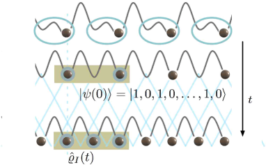
Figure 1: Idealized sketch of the effect of local relaxation in a setting having periodicity $2$. Starting from an idealized initial condition of bosonic atoms being present or absent, $|\psi(0)\rangle=|1,0,\dots,1,0\rangle$, in even and odd sites of a one-dimensional Bose-Hubbard system–achieved by imposing a superlattice to the one-dimensional optical lattice–the system locally relaxes to an apparent maximum entropy state.

II Experimental setup: Ultracold atoms in optical superlattices

The current surge of interest in the relaxation of quantum systems after a quench is mainly motivated by the advent of ultracold atoms in optical lattices [52–56]. These systems are highly attractive as they allow for sudden controlled manipulations of system parameters, hence quenches, are strongly interacting, hence non-trivial, are on experimental time scales essentially closed quantum systems, and therefore show coherent quantum dynamics. Systems are also sufficiently large to show non-trivial many-body behavior.

In the present context, however, the major drawback of ultracold atoms is that despite the unprecedented possibilities of manipulation the study of local relaxation provides an experimental challenge. This is due to the fact that local (i.e., site-resolved) measurements on ultracold atoms in optical lattices are still not satisfactory, albeit rapid progress is being made. In this work, we propose to study instances of local relaxation even in a setting where strictly local quantities can not easily be studied by using optical superlattices [57–60].

Following the setup very recently realized by Bloch and coworkers Wells ; TimeResolved , we consider bosonic Rubidium-87 atoms in a period-$2$ optical superlattice geometry: Two standing-wave laser fields at wavelengths $765$nm and $1530$nm are superimposed with fixed relative location to provide a superlattice geometry of lattice constants $a=382.5$nm and $2a=765$nm. It is experimentally possible, among other things, to (i) change the relative strength of the two optical lattices and (ii) shift their relative position, by altering phase and detuning of the optical superlattice. Assuming the strength of the lattice with lattice constant $a$ to be fixed, (i) allows to couple and decouple this lattice into an array of double well potentials, combining one odd (o) and one even (e) site of the original lattice. In such double well potentials, (ii) allows to introduce a bias between the chemical potentials of the odd and even sites, $\Delta=\mu_{o}-\mu_{e}$.

Isolating double wells and biasing odd vs. even sites, in turn, allows for the preparation of patterns of atoms and for extracting local quantities to the degree that odd and even sites can be distinguished from each other:

• Preparation of periodic patterns is achieved by loading the superlattice while introducing a bias between odd and even sites such that due to a shifting of particles all particles are on either odd or even sites after loading. Using further experimental techniques Wells , multiple occupancies on the occupied sites can be eliminated, leaving a sequence of empty and single-occupied sites.

• Period-$2$ local measurements can be obtained by mapping odd and even sites to different Brillouin zones: Assuming completely decoupled double wells, each part of the double well has multiple bands separated by well-defined energies. Biasing, say, the odd sites relative to the even sites by an energy in excess of the separation energy of the band-separation energy, odd-site particles are reloaded into the higher band of the even sites, whereas the even-site particles stay in the lower band. A standard time-of-flight mapping then shows the even-site particles in the first Brillouin zone, the odd-site particles in the higher Brillouin zones.

• More sophisticated measurements with period-$2$ can also be performed in principle. When letting the system evolve for some defined hold time, and then freezing the time evolution by ramping up the barrier, one can also measure nearest-neighbor correlations in the lattice Wells ; TimeResolved ; Superlattice ; Superlattice2 . There are several ways to proceed here: On the one hand, one can isolate double wells, let them dephase. Then upon free expansion, the average correlations can be measured as in a double slit experiment. One the other hand, correlations can be mapped to densities. To the extent that the barrier between the wells is sufficiently high such that the time evolution can be described by a collection of double well systems (and higher Wannier bands do not have to be taken into account), we can investigate the time evolution in each individual double well. Up to the presence of a confining potential, the total time evolution then reflects the time evolution in each of the double wells. Let us label the two modes in any of the wells by $1$ and $2$, one may apply an appropriate free Hamiltonian to map correlations onto on-site densities. Specifically, for $U=0$ we find that

  $$2\,{\text{im}}\langle\hat{a}_{1}^{\dagger}\hat{a}_{2}\rangle=\langle\hat{a}_{2}^{\dagger}(t)\hat{a}_{2}(t)\rangle-\langle\hat{a}_{1}^{\dagger}(t)\hat{a}_{1}(t)\rangle),$$ (2)

  when letting $\hat{a}_{1},\hat{a}_{2}$ evolve under the free Hamiltonian

  $$\hat{h}=-\left(\hat{a}_{1}^{\dagger}\hat{a}_{2}+\hat{a}_{2}^{\dagger}\hat{a}_{1}\right),$$ (3)

  until $t=\pi/4$. One can hence measure the imaginary part of the appropriate correlators, and hence the period-$2$ correlators in the full lattice. In settings where in the Heisenberg picture the phase map $\hat{a}_{2}\mapsto i\hat{a}_{2}$ for each right well is feasible, one can also measure the real part. If one has small interactions (because of the Wannier band problem—a description in terms of Wannier functions still has to be valid, accompanied by a non-vanishing $U$), then this leads to a small dephasing in this mapping. Direct numerical simulation can take this properly into account, allowing for a correct interpretation of the experimental observation. Such a technique allows to measure correlators from a time-resolved observation of on-site densities. Similar time-resolved measurements have recently been performed in optical superlattices TimeResolved .

As shown in Fig. 1, we propose to start from a two-periodic initial state prepared by the superlattice setup as described above, where all odd sites are occupied by exactly 1 boson and all even sites are empty. The initial state vector of the entire lattice is hence

$$|\psi(0)\rangle=|1,0,1,0,\dots 1,0\rangle.$$ (4)

Tools how to experimentally achieve that sites are to a good approximation occupied by a single atom, and not two or more atoms, are described in Refs. [57–59]. If the $2a$-lattice is suddenly switched off, i.e., the system quenched, the state vector will evolve in time $|\psi(t)\rangle=\mathrm{e}^{-\mathrm{i}t\hat{H}/\hbar}|\psi(0)\rangle$ according to the conventional Bose-Hubbard Hamiltonian

$$\hat{H}=-J\sum_{i=1}^{L}(\hat{b}^{\dagger}_{i+1}\hat{b}_{i}+\hat{b}^{\dagger}_{i}\hat{b}_{i+1})+\frac{U}{2}\sum_{i=1}^{L}\hat{n}_{i}\left(\hat{n}_{i}-1\right),$$ (5)

where $U$ and $J$ are the standard interaction and hopping parameters of the Bose-Hubbard model that can be calculated microscopically from the lattice parameters. The system size is given by $L$, whereas the boson number is $N=L/2$ from this setup. $L$ will always be even in the following, in line with the proposed setup; various boundary conditions will be imposed. We work in units where $J=1$ and $\hbar=1$.

We will not consider the effect of the occupation of higher order bands, but will stay within the limit of applicability of the Bose-Hubbard model. We will for the purposes of the present paper also neither consider an additional harmonic confining potential—except when explicitly stated otherwise—nor additional dephasing effects due to statistical fluctuations of local fields. Instead, we will systematically flesh out what behavior is expected in this slightly idealized setting, to see how local relaxation manifests itself here, to comment on the impact of imperfections later.

As $\hat{\varrho}(0)=|\psi(0)\rangle\langle\psi(0)|$ is not an eigenstate of $\hat{H}$, we are in a non-equilibrium situation. The initial state is uncorrelated and shows inhomogeneous density of periodicity $2$. Coherent quantum dynamics is now expected to homogenize densities locally and to build up non-local correlations.

Local relaxation is now monitored by the global measurement of the total occupation of even, $\langle\hat{N}_{e}(t)\rangle$, and odd, $\langle\hat{N}_{o}(t)\rangle$, sites. In a translationally invariant setting, this gives access to local observables as

$$\langle\hat{N}_{e}(t)\rangle=\sum_{i=1}^{L/2}\bigl{\langle}\hat{n}_{2i}(t)\bigr{\rangle}=\frac{L}{2}\langle\hat{n}_{2i}(t)\rangle,$$ (6)

and similarly for odd sites.

If one has experimental access to the variances $\sigma^{2}_{tot,e,o}=\langle\hat{N}_{tot,e,o}^{2}\rangle-\langle\hat{N}_{tot,e,o}\rangle^{2}$, density-density correlations (see also Ref. NoiseNoise ) between all even and all odd sites may be obtained through

$$\frac{\sigma^{2}_{tot}-\sigma^{2}_{e}(t)-\sigma^{2}_{o}(t)}{2}=\langle\hat{N}_{e}(t)\hat{N}_{o}(t)\rangle-\langle\hat{N}_{e}(t)\rangle\langle\hat{N}_{o}(t)\rangle$$ (7)

$$= \sum_{i,j=1}^{L/2}\left(\langle\hat{n}_{2i}(t)\hat{n}_{2j-1}(t)\rangle-\langle\hat{n}_{2i}(t)\rangle\langle\hat{n}_{2j-1}(t)\rangle\right).$$

In fact, the value of $\hat{N}_{tot}$ is fixed to $L/2$ for the proposed pattern, so in repeated experiments of same length, this quantity will have variance zero, $\sigma_{tot}^{2}=0$.

Moreover, the quasi-momentum distribution defined as

$$S(q,t)=\frac{1}{L}\sum_{i,j=1}^{L}\mathrm{e}^{\mathrm{i}q(i-j)}\left\langle\hat{b}^{\dagger}_{i}(t)\hat{b}_{j}(t)\right\rangle,\;\;\;q\in[0,2\pi],$$ (8)

is also accessible as a global quantity, from time-of-flight measurements.

We now proceed as follows. In order to obtain analytical results we set $U=0$ and $U=\infty$ respectively, which are both essentially non-interacting limiting cases, can be solved exactly and show very similar, but not generally identical results (compare also Ref. LightCone ). These results will be extended to the interacting finite-$U$ case which will be studied using t-DMRG method. For the time-scales considered it is an effectively quasi-exact method.

III Exact solutions for limiting cases

Both limiting cases $U=0$ and $U=\infty$ are or can be mapped to free models. This case has been considered for Gaussian initial conditions in Refs. Tegmark ; Barthel , as well as for non-Gaussian product initial conditions in Ref. Relax . In these cases, the reduced state of a subsystem $I$

$$\hat{\varrho}_{I}(t)={\text{tr}}_{L\backslash I}[\hat{\varrho}(t)]\rightarrow\hat{\varrho}_{\text{max}}.$$ (9)

will converge for large systems and long times to $\hat{\varrho}_{\text{max}}$, being the maximum entropy density operator as constrained by the initial conditions (or, more precisely, if recurrences are considered, this will be true in 1-norm to an arbitrarily small approximation error for an arbitrarily long time). Also, fermionic Gaussian initial states have been considered in Refs. Relax ; Barthel . Local relaxation will therefore happen in these cases.

The physical mechanisms behind the relaxation processes in the cases of $U=0$ and $U=\infty$ is sightly different, however: In the case $U=0$, it is due to dephasing in the sense that freely propagating bosons lead to reduced density operator contributions of quickly oscillating phases that average out. In Ref. Relax , this intuition leads even for non-Gaussian initial states to maximum entropy states, by invoking a quantum version of a central limit theorem, and exploiting the finite speed of information transfer LRC .

In the case $U=\infty$, real scattering processes happen, albeit of a very specific form that allows for a formal mapping to a non-interacting fermionic problem (and to the XX model, compare also Ref. LightCone ): The scattering is simply relegated to the internal sign structure of the wave function. We will also see that the two relaxation processes lead to different time-evolutions of most physical observables.

For all cases of nonzero finite $U$, the situation should be somehow intermediate. For the specific setup chosen here, interacting particles will learn of each others existence only after some initial time they need to come into contact. We would therefore expect that for very short time scales, observables should evolve as in the $U=0$ limit, with a crossover in behavior for longer time scales when they start interacting. The question is whether for which interaction strengths the limiting pictures remain essentially valid and whether there is a genuinely different intermediate interaction regime with different relaxation behavior. Compared to Refs. Relax ; Tegmark ; Barthel , in this work we focus to a lesser extent on rigorous mathematical convergence statements—like invoking quantum versions of central limit theorems—but instead put more emphasis on the phenomenology of the physical relaxation process as such in the $2$-periodic setting.

III.1 Non-interacting bosons: $\mathbf{U=0}$

In the translationally invariant case of non-interacting bosons, the Hamiltonian can be diagonalized by Fourier transforming to new bosonic operators $\hat{a}_{1},\dots,\hat{a}_{L}$ to yield

$$\hat{H}_{U=0}=\sum_{k=1}^{L}\lambda_{k}\hat{a}^{\dagger}_{k}\hat{a}_{k},$$ (10)

where

$$\lambda_{k}=-2\cos(2\pi k/L)$$ (11)

are the eigenvalues of the circulant Hamilton matrix $H$ with entries $H_{i,j}=-\delta_{\text{dist}(i,j),1}$. While the real experiment will not have periodic boundary conditions, our calculations show that for realistic system sizes and time scales the difference between open and periodic boundary conditions is negligible.

In the Heisenberg picture, the initial state vector $|\psi(0)\rangle=|1,0,\dots,1,0\rangle$ remains time-independent, whereas the operators evolve in time as

$$\begin{split}\hat{b}_{i}(t)&=\sum_{j=1}^{L}V_{i,j}(t)\hat{b}_{j}(0),\;\;\;V(t)=\mathrm{e}^{-\mathrm{i}tH},\\ V_{i,j}(t)&=\frac{1}{L}\sum_{k=1}^{L}\mathrm{e}^{-\mathrm{i}t\lambda_{k}}\mathrm{e}^{2\pi\mathrm{i}k(i-j)/L}.\end{split}$$ (12)

Straightforward algebra then yields the exact time-evolution of two-point correlations, see Appendix,

$$\begin{split}f_{i,j}&=\left\langle\hat{b}_{i}^{\dagger}(t)\hat{b}_{j}(t)\right\rangle\\ &=\frac{1}{2}\delta_{i,j}-\frac{(-1)^{i}}{2}V_{j,i}(2t).\end{split}$$ (13)

In the thermodynamic limit $L\rightarrow\infty$ this turns into

$$f_{i,j}=\frac{1}{2}\delta_{i,j}-\frac{(-1)^{i}\mathrm{i}^{j-i}}{2}J_{j-i}(4Jt),$$ (14)

where $J_{n}$ is a Bessel function of the first kind.

From the above expression, one can derive the quasi-momentum distribution for finite $L$, see Appendix. For $Lq/(2\pi)\in\{1,\dots,L\}$ it is constant, $S(q,t)=1/2$, while one finds

$$S(q,t)=\frac{1}{2}+\frac{\mathrm{i}}{L^{2}}\sum_{p=1}^{L}\mathrm{e}^{4J\mathrm{i}t\cos(2\pi p/L)}\frac{\sin^{2}(Lq/2)}{\sin(2\pi p/L-q)}.$$ (15)

for all other $q\in[0,2\pi]$.

With slightly more effort, density-density correlations as in Eq. (7) emerge as (see Appendix)

$$\langle\hat{n}_{2i}(t)\hat{n}_{2j-1}(t)\rangle-\langle\hat{n}_{2i}(t)\rangle\langle\hat{n}_{2j-1}(t)\rangle\hskip 56.9055pt$$ (16)

$$=f_{2i,2j-1}f_{2j-1,2i}-2\sum_{k=1}^{L/2}|V_{2i,2k-1}(t)V_{2j-1,2k-1}(t)|^{2},$$

which, as they are local quantities, relax for large systems and long times. For large $L$ one finds for the global density-density correlator (see Appendix)

$$\begin{split}&\langle\hat{N}_{e}(t)\hat{N}_{o}(t)\rangle-\langle\hat{N}_{e}(t)\rangle\langle\hat{N}_{o}(t)\rangle\\ &\hskip 11.38092pt\rightarrow-\frac{L}{16}\left(3+J_{0}(8Jt)-4[J_{0}(4Jt)]^{2}\right).\end{split}$$ (17)

We also show in detail the exact local relaxation to a maximum entropy state for the case of the initial condition $|\psi(0)\rangle=|1,0,\dots,1,0\rangle$, largely following Ref. Relax : For every block of consecutive sites $I=\{1,\dots,s\}$, every small error $\varepsilon>0$ and any desired, arbitrarily long recurrence time $t_{\text{rec}}>0$ there exists a system size $L$ and a local relaxation time $t_{\text{rel}}>0$ such that

$$\|\hat{\varrho}_{I}(t)-\hat{\varrho}_{\text{max}}\|_{1}<\varepsilon$$ (18)

for all times $t\in[t_{\text{rel}},t_{\text{rec}}]$, see Appendix. Here, $\|\cdot\|_{1}$ denotes the trace norm. Hence, after the quench for $U=0$, for $2$-periodic initial conditions, the local state becomes in time a maximum entropy state, to an arbitrarily good approximation.

III.2 Hardcore bosons: $\mathbf{U\rightarrow\infty}$

In the limit $U\rightarrow\infty$, the interaction manifests itself exclusively in that bosonic occupation numbers are upper bounded by $1$. This leads to a well-known mapping in case of quantum ground states: The hard core limit is equivalent to the XX spin model and a model of spinless free fermions. But even in time evolution, in the limit of large $U$, the population of sites with particle number larger than unity is dynamically suppressed to an arbitrary extent: The expectation value of the new Hamiltonian is obviously preserved under time evolution, $\text{tr}[\hat{H}\hat{\varrho}(0)]=\text{tr}[\hat{H}\hat{\varrho}(t)]$, $H=-\hat{H}_{0}+U\hat{H}_{1}$, where

$$\hat{H}_{0}=\sum_{i=1}^{L}(\hat{b}^{\dagger}_{i+1}\hat{b}_{i}+\hat{b}^{\dagger}_{i}\hat{b}_{i+1}),\,\hat{H}_{1}=\frac{1}{2}\sum_{i=1}^{L}\hat{n}_{i}\left(\hat{n}_{i}-1\right).$$ (19)

For initial states that are supported on span$(|0\rangle,|1\rangle)$ one has $\text{tr}[\hat{H}\hat{\varrho}(0)]=-\text{tr}[\hat{H}_{0}\hat{\varrho}(0)]$. Furthermore $\text{tr}[\hat{H}\hat{\varrho}(t)]\geq\text{tr}[(-\hat{H}_{0}+U\hat{H}_{2})\hat{\varrho}(t)]$, where

$$\hat{H}_{2}=\sum_{i=1}^{L}\sum_{k=2}^{\infty}|k\rangle\langle k|,$$ (20)

where the latter projector defined on each site $i$. This, in turn, means that

$$\frac{\text{tr}[\hat{H}_{0}(\hat{\varrho}(t)-\hat{\varrho}(0))]}{U}\geq\text{tr}[\hat{H}_{2}\hat{\varrho}(t)]\geq 0.$$ (21)

Hence, one can ensure to arbitrary accuracy for large $U$ that $\hat{\varrho}(t)$ is only supported on $\text{span}(|0\rangle,|1\rangle)$. One therefore arrives in a perfectly meaningful way at the familiar hard core limit of the Bose-Hubbard model, which is equivalent to a free fermionic spinless system.

This mapping to non-interacting spinless fermions is done through the familiar Jordan-Wigner transformation

$$\hat{b}_{n}=\mathrm{e}^{-\mathrm{i}\pi\sum_{m<n}\hat{c}^{\dagger}_{m}\hat{c}_{m}}\hat{c}_{n}.$$ (22)

Under this transformation the initial state vectors turn into

$$|\psi\rangle=\hat{c}_{1}^{\dagger}(0)\hat{c}_{3}^{\dagger}(0)\hat{c}_{5}^{\dagger}(0)\ldots|0\rangle$$ (23)

and the Hamiltonian reads upon a Fourier transformation to new fermionic operators $\hat{d}_{1},\dots,\hat{d_{L}}$

$$\hat{H}_{U=\infty}=\sum_{k=1}^{L}\lambda_{k}\hat{d}^{\dagger}_{k}\hat{d}_{k}$$ (24)

with $\lambda_{k}$ as in Eq. (11) and the time-evolution of the operators is given by

$$\hat{c}_{i}(t)=\sum_{j=1}^{L}V_{i,j}(t)\hat{c}_{j}(0)$$ (25)

with $V_{i,j}(t)$ as in Eq. (12). This is formally identical to the $U=0$ case. However, there are two differences: Periodic boundary conditions in the original bosonic model map to (anti-)periodic boundary conditions $\hat{c}^{\dagger}_{L+1}=(-1)^{N+1}\hat{c}^{\dagger}_{1}$. Hence, boundary conditions stay periodic if the particle number $N$ is odd, to which we restrict ourselves in the following.

The second, more important difference is that differences in results will show up due to the Jordan-Wigner transformation of operators and the difference between bosonic and fermionic (anti)commutators. It is easily shown that local densities and correlations between nearest neighbors translate directly (see XIII.4), such that the respective results for $U=\infty$ are identical to those for $U=0$. For longer-ranged two-point correlations, including structure functions, as well as density-density correlations results differ. Density-density correlations are given by (see XIII.4)

$$\begin{split}\langle\hat{n}_{2i}(t)\hat{n}_{2j-1}(t)\rangle-\langle\hat{n}_{2i}(t)\rangle\langle\hat{n}_{2j-1}(t)\rangle\hskip 56.9055pt\\ =-f_{2i,2j-1}f_{2j-1,2i},\end{split}$$ (26)

where $f_{i,j}$ is as in Eq. (13). For large $L$ the global density-density correlator is then given by (see Appendix)

$$\begin{split}&\langle\hat{N}_{e}(t)\hat{N}_{o}(t)\rangle-\langle\hat{N}_{e}(t)\rangle\langle\hat{N}_{o}(t)\rangle\\ &\rightarrow-\frac{L}{16}\left(1-J_{0}(8Jt)\right).\end{split}$$ (27)

III.3 Interacting softcore bosons: Finite $\mathbf{U}$

In this case, we are no longer facing an integrable model. In order to study the relaxation dynamics, we will therefore turn to the time-dependent variant VidalTEBD ; Daley ; WhiteFeiguin of the DMRG (density-matrix renormalization group) method White ; RMP . This method allows to follow the coherent time-evolution of strongly interacting quantum systems very precisely. Its reach in time is, however, limited by the growth of entanglement in quantum systems: Linear entanglement growth, for example, leads to an exponential growth in numerical resources needed. As we will see, interestingly, the system under study is characterized by very strong linear entanglement growth. In the free instances this linear increase is indeed provably correct Relax ; Schuch , see Sec. IX. Hence, the reachable times are quite short ($Jt\approx 6$) with up to $5000$ states kept in the simulations. For most quantities, this turns out to be sufficiently long to make contact to the non-interacting results and to read off long-time behavior. In particular, the results allow for a quantitative comparison to experiments.

A subtlety arises from the fact that DMRG prefers open boundary conditions, and is hence closer to experiment. However, we would like also to compare to analytical results, where periodic boundary conditions are preferable. As it will turn out, for system sizes and times considered, the difference is negligible.

IV Time evolution of densities

For the time evolution of local densities both exactly solvable cases $U=0$ and $U=\infty$ give the same result

$$\begin{split}\left\langle\hat{n}_{i}(t)\right\rangle&=\frac{1}{2}-\frac{(-1)^{i}}{2L}\sum_{k=1}^{L}\mathrm{e}^{4\mathrm{i}tJ\cos(2\pi k/L)}\\ &\rightarrow\frac{1}{2}-\frac{(-1)^{i}}{2}J_{0}(4Jt)\quad(L\rightarrow\infty).\end{split}$$ (28)

Odd- and even-site densities relax symmetrically about the $n=1/2$ axis to $n=1/2$, with an asymptotic decay as $t^{-1/2}+o(t^{-1/2})$.

All $t$-DMRG results for finite $U$ are perfectly compatible with relaxation of local densities to $n=1/2$. On very short time scales ($t<1$) particles have typically not collided yet and are not yet sensitive to the values of $U$, hence, finite $U$ results are identical to the limiting cases $U=0,\infty$. The relaxation behavior for intermediate times, however, deviates quite strongly. Interaction effects become visible right after particles make contact. This can be seen in Figs. 2-6 (all calculated for $L=32$), where we compare the time evolution of local densities for various finite values of $U$ to the special cases $U=0,\infty$. For small $U$ (exemplified by $U=1.5$) and large $U$ (exemplified by $U=8$), the comparison indicates that the relaxation of local densities is governed by the behavior of the limiting non-interacting cases. For intermediate values of $U$ (exemplified by $U=3$), scattering seems to be most effective and lead to much faster damping and relaxation, much beyond the above square root time dependence. This is plausible, as close to a quantum critical model there is a limiting point in the spectrum of the new Hamiltonian, leading to specifically effective relaxation. Deviations from the limiting behavior are sufficiently strong that they should be visible experimentally.

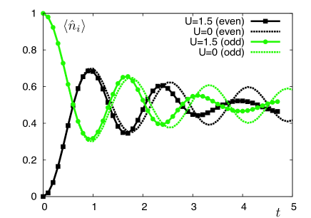
Figure 2: Local density $\langle\hat{n}_{i}(t)\rangle$ vs. time, showing local relaxation. Shown is the time evolution of an even and an odd site for $U=0$ and $U=1.5$.

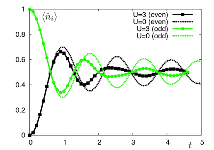
Figure 3: Local density $\langle\hat{n}_{i}(t)\rangle$ vs. time, showing local relaxation. Shown is the time evolution of an even and an odd site for $U=0$ and $U=3$. Note the strong deviation from the non-interacting limit and the strong suppression of density oscillations.

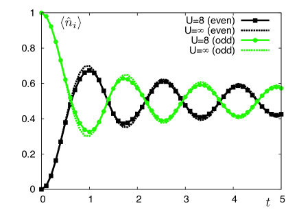
Figure 4: Local density $\langle\hat{n}_{i}(t)\rangle$ vs. time, showing local relaxation. Shown is the time evolution of an even and an odd site for $U=8$ and $U=\infty$. The agreement is almost perfect.

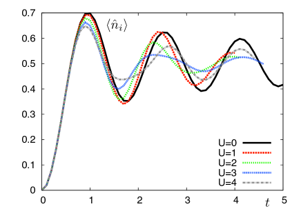
Figure 5: Time evolution of local densities on even sites for various $U$ compared to the limiting behavior $U=0$.

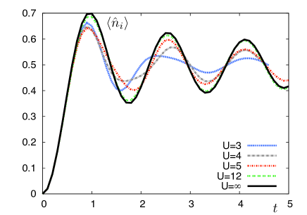
Figure 6: Time evolution of local densities on even sites for various $U$ compared to the limiting behavior $U=\infty$.

Under the assumption that for the time scales achievable by DMRG an asymptotic power-law can already be read off, one finds the exponents given in Fig. 7. While for very small $U$ and all $U>4$ one finds a slope similar to $t^{-1/2}$, as for the limiting cases, there is an intermediate regime where relaxation is much faster. It must be stated, however, that in this regime the precise slope is hard to extract, even an exponentially fast decay cannot be excluded completely, but we are not aware of a physical reason why there should be a qualitative change of decay behavior from power-law to exponential. Qualitatively, stronger interactions should lead to a more distinct dispersion, leading in turn to a quicker decay.

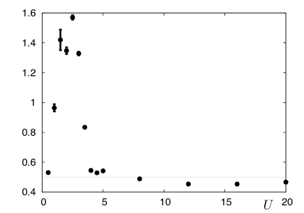
Figure 7: Estimated negative exponents of asymptotic power-law decay law for local densities. The asymptotic decay exponent for the limiting cases is shown as a dashed line.

Concerning experimental implementations, a number of further issues require a discussion: The experimentally accessible systems will be of finite size, leading to recurrence effects. Moreover, there will be a parabolic confining potential, which will modify results. Furthermore, one will encounter initial states at non-zero temperature, as well as possible additional fluctuations due to inhomogeneities in applied fields, different from the apparent local relaxation.

So far, we have confronted analytical results in the $L\rightarrow\infty$ limit with DMRG results for $L=32$. In order to check whether on the time scales reachable by DMRG recurrence effects can be seen for this system size, we have rerun selected calculations for $L=50$, observing no relative change in results above 1 percent. In particular, the shapes of oscillatory behavior remained completely unchanged. In the $U=0$ limit, finite system DMRG results and infinite as well as finite system analytic results agree completely on the finite times reachable by DMRG, even despite the different boundary conditions (open boundary conditions (OBC) for DMRG, periodic boundary conditions (PBC) for analytical statements). Recurrences, where the difference between finite and infinite system becomes obvious, happen much later, see Fig. 8.

The effect of the trap, as shown in Fig. 10, is to generate effective reflections from the edges of the system, leading to much earlier recurrences. However, in experimental setups, this effect would for realistic traps set in late enough to allow for sufficiently long observation.

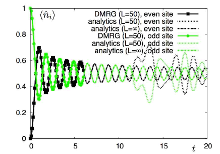
Figure 8: Densities in the free limit: Analytics for $L=50$ (PBC), $L=\infty$ (PBC) and DMRG for $L=50$ (OBC; in fact calculated in the hardcore limit, because DMRG fails for $U=0$, but densities are identical in both cases). On the time scales reached by DMRG, all three agree. This incidentally shows that boundary conditions are of little importance for the sizes and time scales of DMRG. Recurrence effects become visible later.

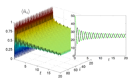
Figure 9: Density $\langle\hat{n}_{i}(t)\rangle$ (left) for $U=0$, $L=100$, and periodic boundary conditions. The plot on the right shows $\langle\hat{N}_{e}(t)\rangle$ (black) and $\langle\hat{N}_{o}(t)\rangle$ (green), compare Fig. 10, where the same is shown including a trapping potential.

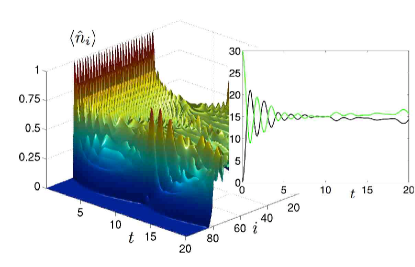
Figure 10: Density $\langle\hat{n}_{i}(t)\rangle$ (left) for $U=0$, $L=100$, including a trapping potential corresponding to a local chemical potential $\mu_{i}=0.01(i-L/2)^{2}$. The plot on the right shows $\langle\hat{N}_{e}(t)\rangle$ (black) and $\langle\hat{N}_{o}(t)\rangle$ (green). Note the similarity to a Bessel function for short times and the recurrences after $t\approx 10$. The recurrences are even more pronounced in the quasi-momentum distribution, Fig. 18, which lacks, however, signatures of local relaxation dynamics.

V Time evolution of local correlators

Let us now consider the nearest-neighbor correlator $\langle\hat{b}^{\dagger}_{i+1}(t)\hat{b}_{i}(t)\rangle$. This quantity is specifically interesting, and can in principle be measured by means of exploiting the tuning of the double well potential of the superlattice, and appropriate timing (see above, and compare also Refs. Wells ; TimeResolved ; Superlattice ). It is of interest as it goes beyond local densities: The build-up of correlations in time starting from the uncorrelated initial state becomes visible.

In the limiting free cases, identical results are found:

$$\begin{split}\left\langle\hat{b}^{\dagger}_{i+1}(t)\hat{b}_{i}(t)\right\rangle&=\frac{(-1)^{i}}{2L}\sum_{k=1}^{L}\mathrm{e}^{4Jt\mathrm{i}\cos(2\pi k/L)}\mathrm{e}^{-2\pi\mathrm{i}k/L}\\ &\rightarrow-\frac{(-1)^{i}}{2\mathrm{i}}J_{1}(4Jt)\quad(L\rightarrow\infty).\end{split}$$ (29)

The real part of the correlator is strictly zero for all times, whereas the imaginary part relaxes to $0$ with an asymptotics of $t^{-1/2}$ after a quick growth to a maximal value of about $0.28$ at time $t\approx 1/2$. This quick growth reflects the buildup of correlations due to particle motion with speed linear in $J$.

For finite $U$, the scenario has marked similarities and differences. Considering Figs. 11 and 12, one sees that on short time scales the buildup of the imaginary part of correlations is identical for arbitrary $U$. This simply reflects the fact that due to the distance $2$ between particles at $t=0$, no collisions have yet happened on these time scales. Only when the interaction strength becomes visible, the relaxation to 0 follows different paths. As for local densities there is a clear trend that relaxation is fastest around $U\approx 3$, reflecting the particularly efficient scattering there. In the real part, convergence to a finite value occurs for all finite $U$, but not such a clear picture of relaxation speeds occurs.

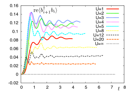
Figure 11: Real part of correlations to neighbors $\langle\hat{b}_{i+1}^{\dagger}(t)\hat{b}_{i}(t)\rangle$ as a function of time, for different values of $U$. Note that in the effectively free cases $U=0$ and $U=\infty$, the absolute value of these correlators converges to zero.

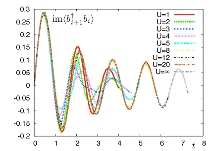
Figure 12: Imaginary part of correlations to neighbors $\langle\hat{b}_{i+1}^{\dagger}(t)\hat{b}_{i}(t)\rangle$ as a function of time, for different values of $U$.

If one plots the asymptotic values of the real part of the nearest neighbor correlators (Fig. 13), one sees that there is a maximum around $U\approx 3$, reflecting the efficient scattering there. Interestingly, the large-$U$ behavior can be very well approximated by a $U^{-1}$ curve for all $U=4$ and larger.

Indeed, this dependence is exactly what one would expect in the thermal or Gibbs state of the Bose-Hubbard Hamiltonian $\hat{H}$: We hence look at local correlations in the Gibbs state

$$\hat{\varrho}_{\beta}=\mathrm{e}^{-\beta\hat{H}}/Z$$ (30)

with $Z=\text{tr}[\mathrm{e}^{-\beta\hat{H}}]$ . We will take

$$\hat{H}_{0}=\frac{U}{2}\sum_{i=1}^{L}\hat{n}_{i}\left(\hat{n}_{i}-1\right).$$ (31)

as our unperturbed Hamiltonian including interactions and look at leading orders in the hopping term

$$\hat{V}=-J\sum_{i=1}^{L}(\hat{b}^{\dagger}_{i+1}\hat{b}_{i}+\hat{b}^{\dagger}_{i}\hat{b}_{i+1}).$$ (32)

Then we find, using standard thermal perturbation theory, up to first order in $J$

$$\begin{split}\langle\hat{b}_{i}^{\dagger}\hat{b}_{j}\rangle&=\delta_{i,j}\langle\hat{b}_{i}^{\dagger}\hat{b}_{i}\rangle-\int_{0}^{\beta}\!\!\!\!\mathrm{d}x\,\frac{\text{tr}[\mathrm{e}^{(x-\beta)\hat{H}_{0}}\hat{V}\mathrm{e}^{-x\hat{H}_{0}}\hat{b}_{i}^{\dagger}\hat{b}_{j}]}{Z}.\end{split}$$ (33)

This means that we have ($\delta_{\langle i,j\rangle}=1$ if $i$ and $j$ are nearest neighbors, zero otherwise)

$$\langle\hat{b}_{i}^{\dagger}\hat{b}_{j}\rangle=\delta_{i,j}\langle\hat{b}_{i}^{\dagger}\hat{b}_{i}\rangle\hskip 156.49014pt$$ (34)

$$+\delta_{\langle i,j\rangle}\frac{J}{U}\sum_{n,m}\mathrm{e}^{-\beta(E_{n}+E_{m})}n(m+1)\frac{\mathrm{e}^{\beta U(n-m-1)}-1}{z^{2}(n-m-1)}$$

where $z=\sum_{n}\mathrm{e}^{-\beta E_{n}}$ and $E_{n}=Un(n-1)/2$ are the local energies of the unperturbed Hamiltonian. So, indeed, within the validity of perturbation theory, we do find the anticipated linear dependence on $1/U$, as seen also in DMRG simulations in the time-dependent scenario. By definition, the correlators merely probe local quantities. This corroborates the intuition that locally, the system is indistinguishable from the situation as if globally the system was in a state maximizing the entropy, under the constraints of motion Relax ; Tegmark ; Barthel .

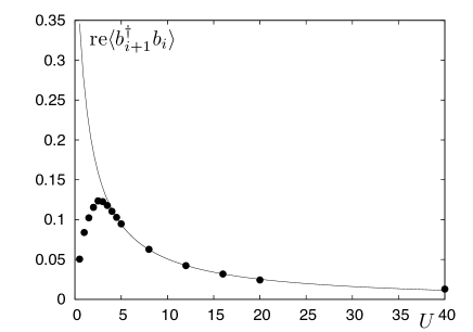
Figure 13: Equilibrated value of the real part of correlations to neighbors $\langle\hat{b}_{i+1}^{\dagger}(t)\hat{b}_{i}(t)\rangle$ for large $t$ for different values of $U$. As a guide to the eye, large-$U$ behavior is fitted by a solid line proportional to $1/U$.

To complete the picture, let us finally remind ourselves of how the maximum entropy states of the global system locally look like. The constants of motion of interest here are the occupation numbers in bosonic or fermionic momentum space, respectively. The global maximum entropy state—under the constraints of motion—for $U=0$ is then found to be

$$\hat{\varrho}=\bigotimes_{i=1}^{L}\frac{2}{3}e^{-\ln(3)\hat{b}^{\dagger}_{i}\hat{b}_{i}}.$$ (35)

This result is completely consistent with our result for the relaxation of the characteristic function (see Appendix XIII.2). One can now calculate expectation values in equilibrium for the local observables considered above (by construction in agreement with our earlier analytical findings) as

$$\langle\hat{b}^{\dagger}_{i}\hat{b}_{j}\rangle=\frac{1}{2}\delta_{i,j},\,\langle\hat{n}_{i}\hat{n}_{j}\rangle-\langle\hat{n}_{i}\rangle\langle\hat{n}_{j}\rangle=\frac{3}{4}\delta_{i,j}.$$ (36)

In the case of $U\rightarrow\infty$ one finds

$$\hat{\varrho}=\frac{1}{2^{L}}{\mathbbm{1}},$$ (37)

which means that

$$\langle\hat{b}^{\dagger}_{i}\hat{b}_{j}\rangle=\frac{1}{2}\delta_{i,j},\,\,\langle\hat{n}_{i}\hat{n}_{j}\rangle-\langle\hat{n}_{i}\rangle\langle\hat{n}_{j}\rangle=\frac{1}{4}\delta_{i,j}.$$ (38)

We have also numerically investigated the relaxation behavior of longer-ranged correlators $\langle\hat{b}_{j}^{\dagger}(t)\hat{b}_{i}(t)\rangle$. As an example, we depict in Fig. 14 the relaxation of the real part of $\langle\hat{b}_{i+2}^{\dagger}(t)\hat{b}_{i}(t)\rangle$, the imaginary part being zero. Relaxation here is of monotonically increasing effectiveness with $U$. The relaxation dynamics for $U=0$ and $U=\infty$ is different, revealing the fundamentally different character of the non-interacting limiting cases.

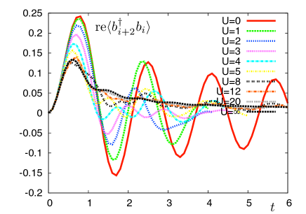
Figure 14: Real part of correlations to neighbors $\langle\hat{b}_{i+2}^{\dagger}(t)\hat{b}_{i}(t)\rangle$ as a function of time, for different values of $U$.

VI Local relaxation

Let us summarize the properties of local relaxation that can be extracted in this experimental setup. In all quantities, there are three time regimes:

1. The first time regime is associated with the building up of correlations: This is governed directly by the coupling strength to the nearest neighbor, and on the shortest times is identical for all $U$, before collision processes become important. The time scale is $Jt<1$, as this is when the first collisions happen and establish correlations.

2. The second time regime is associated with local relaxation. There is fast oscillating dynamics between neighboring sites, happening at a time scale dictated by the hopping $J$, which also governs the speed of sound. Local relaxation as such is slow, in the exact analysis a slow polynomial decay: The Bessel function fulfills $|J_{0}(x)|\leq x^{-1/3}$ as a strict bound, with an asymptotic envelope

   $$J_{0}(x)=x^{-1/2}+o(x^{-1/2}).$$ (39)

   one finds relaxation (not due to decoherence but due the dilution of information over the lattice) to the true local equilibrium. For finite $U$, numerics is consistent with polynomial decay, which for intermediate $U$ seems to be much faster, but still polynomial.

   The intuition is that this local relaxation is due to influences of excitations travelling with the speed of information propagation from farther and farther lattice sites, broadened by dispersion. This means that this time scale, even in the interacting case of $U>0$, should be defined by the speed of information propagation in the system. Note that to date, there is no rigorous bound known to the speed of information propagation in the fully interacting Bose-Hubbard model (this being a consequence of the lattice sites having an unbounded number of particles, see also comments in Refs. Nachtergaele ; HarmonicLiebRobinson ; Buer ). On physical grounds, yet, it should be expected to be similar to $J$, i.e. ”ballistic” transport at the high energies provided by the quench, slightly modified by $U$ (possibly the resulting bounds can only be formulated for specific initial states having small local particle number). This is also what the numerics shows. Note that the low-energy speed of sound need not be relevant here.

3. The third (very large) time is the recurrence time, which seems to be shortened substantially in the presence of a realistic trap. As in the presence of a trap, the excitations no longer travel with a constant speed (the speed of sound), but are slowly reflected, one should expect a quicker relaxation, and this is also the behavior the analytics exhibits. Generally, for moderate to large system sizes it is already beyond the reach of our simulations. It would be interesting to see, possibly in exact diagonalization, whether the recurrences are weakened compared to the free solutions due to interactions in the system, see also Ref. LightCone .

While these findings are essentially independent of the interaction strength $U$, we also find three local relaxation regimes for different $U$:

• For very small values of $U$ (up to $U\approx 1$) relaxation dynamics is quite close to the non-interacting bosonic limit.

• For larger values of $U$ the system seems to show a behavior very similar to the hard core bosonic or free fermionic limit with similar relaxation exponents of order $1/2$. Local correlations are consistent with locally equilibrated subsystems perturbatively coupled in $1/U$.

• The case of intermediate $U\sim 3$ appears to be a special case for various observables, marking the “boundary” between the “free bosonic case” $U=0$ and the “hard core boson case” $U=\infty$, so the fermionic one. Collisions lead to the most efficient relaxation in this case.

To summarize, the dynamics of local quantities shown is consistent with the limiting $U=0$ and $U=\infty$ cases, but shows a richer phenomenology in particular for intermediate $U$.

VII Quasi-momentum distribution

In this subsection, we briefly compare what is seen in the above local relaxation with the situation in momentum space. The quasi- momentum distribution,

$$S(q,t)=\frac{1}{L}\sum_{i,j=1}^{L}\mathrm{e}^{\mathrm{i}q(i-j)}\langle\hat{b}_{i}^{\dagger}(t)\hat{b}_{j}(t)\rangle,$$ (40)

obtainable from time-of-flight experiments, is no longer a local quantity, but a global one probing the state of the entire lattice, as well as the boundary conditions and possibly a confining additional potential. In fact, in the free model for $U=0$, one finds that the quasi-momentum distribution will be very little time-dependent, and if so, in a chaotic fashion showing little structure, see Fig. 17. More specifically, we find (see Appendix) $S(q,t)=1/2$ for $q=2\pi l/L$, $l=1,\ldots,L$, and

$$S(q,t)=\frac{1}{2}+\frac{\mathrm{i}}{L^{2}}\sum_{p=1}^{L}\mathrm{e}^{4J\mathrm{i}t\cos(2\pi p/L)}\frac{\sin^{2}(Lq/2)}{\sin(2\pi p/L-q)}.$$ (41)

for all other $q\in[0,2\pi]$. In case of $U=0$, the quasi-momentum distribution hence indeed does not show any signatures of the local dynamics, see Fig. 17. This is, again, not inconsistent at all with the notion of local relaxation: This quantity is a global one (and local only insofar as correlators of far away lattice sites are suppressed via a quickly rotating exponential function). For any subblock, the dynamics drives the system towards the values of equilibrium. In momentum space, this is not necessarily the case; at least not on these time scales. In the free situation of $U=0$, this leads to an absence of relaxation of this quantity.

It would still be interesting to measure this quantity for close to free cases for short times, to demonstrate the very point that the information about the initial condition is fully contained in the system, and merely diluted. Hence, obviously, one cannot expect true global relaxation to happen, unless a further mechanism of decoherence due to additional external degrees of freedom is present.

In Fig. 18 we show the quasi-momentum distribution for the situation including a trapping potential. The effect of the additional harmonic potential is very significant. Yet, again, note the absence of signatures of the time scales of local dynamics as compared to Figs. 9, 10.

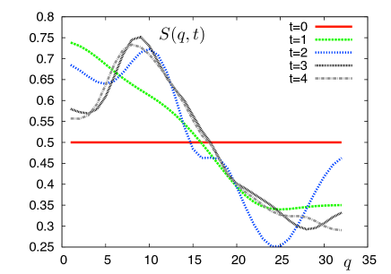
Figure 15: Quasi-momentum distribution as a function of time, for $U=1.5$. The labels $q$ on the $x$-axis correspond to momenta ${\pi}/({L+1})q$, best suited to DMRG open boundary conditions, as explained in the text.

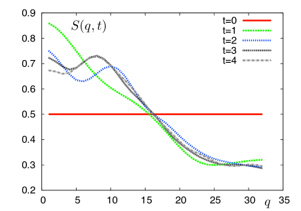
Figure 16: Quasi-momentum distribution as a function of time, for $U=3$, marking the cross-over regime. Labels as in Fig. 15.

How does this compare to the case of having a finite on-site interaction $U$? Again, the behavior reminds of the situation in the free case of $U=0$. The quantity is too non-local to grasp the effect of local relaxation. Still, for longer times, one may also expect relaxation in some translationally invariant properties in momentum space, and the quasi-momentum distribution may well relax. Such a situation is observed in a flow equations approach in case of an interacting model in Ref. Moeckel . For the DMRG calculations we use a slightly different definition of the quasi-momentum distribution

$$S(q,t)=\frac{2}{L+1}\sum_{i,j=1}^{L}\sin\left[\frac{\pi qi}{L+1}\right]\sin\left[\frac{\pi qj}{L+1}\right]\langle\hat{b}^{\dagger}_{i}(t)\hat{b}_{j}(t)\rangle.$$ (42)

This ensures that $S(q,t)$ is a constant of motion for $q=1,\dots,L$ in the free system $(U=0)$ in case of OBC. Fig. 15 and Fig. 16 show this quasi-momentum distribution for $q=1,\dots,L$ for different values of $U$. Indeed, signatures of such a behavior are also observed in Fig. 15, where the momentum distribution is depicted for different values of time $t$. For larger times, the quasi-momentum distribution appears to relax in the interacting case of $U=1.5$. This effect is even more distinct in the case of stronger interactions, as depicted in Fig. 16.

To reiterate, the very absence of relaxation in close to free settings on short times gives rise to an interesting situation: One could experimentally see signatures of local relaxation. One could, however, also see that the information becomes more and more dilute in position space, but is still preserved in the system as such, as seen in the quasi-momentum distribution.

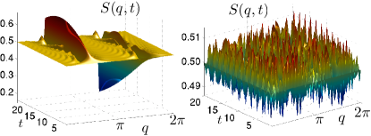
Figure 17: Quasi-momentum distribution $S(q,t)$ for $U=0$, $L=100$, and open (left), periodic (right) boundary conditions. Note the dramatic difference between open/periodic boundary conditions and the absence of the time-scales clearly visible for local observables as in Figs. 9, 10: The fast oscillatory behavior and the relaxation time. See Fig. 18 for $S(q,t)$ in the presence of a trap. The non-local quantity of the quasi-momentum distribution detects the boundary conditions early.

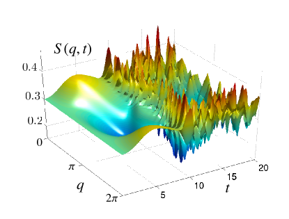
Figure 18: Quasi-momentum distribution $S(q,t)$ for the same parameters as in Fig. 10. Note the absence of the time-scales clearly visible for local observables as in Figs. 9, 10: The fast oscillatory behavior and the relaxation. The recurrence is however clearly visible.

VIII Global density-density correlator

One potentially experimentally accessible global correlator is the connected density-density correlator

$$\langle\hat{N}_{e}(t)\hat{N}_{o}(t)\rangle-\langle\hat{N}_{e}(t)\rangle\langle\hat{N}_{o}(t)\rangle$$ (43)

which we show for different $U$ in Fig. 19. Numerics indicates that this quantity looks effectively relaxed after some time as long-range correlators contributing will be small. For the free case of $U=0$, one analytically finds for large $L$ (see Appendix)

$$\begin{split}&\langle\hat{N}_{e}(t)\hat{N}_{o}(t)\rangle-\langle\hat{N}_{e}(t)\rangle\langle\hat{N}_{o}(t)\rangle\\ &\hskip 11.38092pt\rightarrow-\frac{L}{16}\left(3+J_{0}(8Jt)-4[J_{0}(4Jt)]^{2}\right),\end{split}$$ (44)

which relaxes to $-3L/16$ for large times. For hardcore bosons the global density-density correlator for large $L$ is given by

$$\begin{split}&\langle\hat{N}_{e}(t)\hat{N}_{o}(t)\rangle-\langle\hat{N}_{e}(t)\rangle\langle\hat{N}_{o}(t)\rangle\\ &\rightarrow-\frac{L}{16}\left(1-J_{0}(8Jt)\right),\end{split}$$ (45)

which relaxes to $-L/16$ for large times.

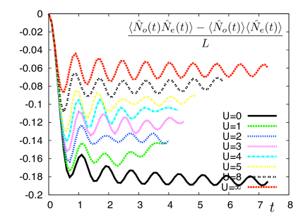
Figure 19: Global density-density correlations for a system of length $L=32$ for various interaction strengths $U$.

IX Entanglement and entropy growth

The creation of excitations at all points of the lattice will in general create a significant degree of entanglement in the time evolving state. Since at each site, an excitation starts to travel through the lattice, a linear increase of the entanglement entropy of subblocks in time is to be expected Entanglement0 ; Entanglement ; Entanglement2 . More precisely, it has been shown in Refs. Entanglement ; Entanglement2 that for any time evolution under a local Hamiltonian with finite-dimensional constituents, starting from a product state, the entanglement entropy of a subblock $I=\{1,\dots,s\}$ grows in one-dimensional systems in $s$ at most as

$$E(\hat{\varrho}_{I}(t))\leq c_{0}t+c_{1},$$ (46)

for suitable constants $c_{0},c_{1}$. This means that for any constant time, the entanglement entropy satisfies what is called an area law. For larger and larger block sizes, the entanglement entropy will eventually saturate in $s$ (and, e.g., not logarithmically diverge).

In turn, this upper bound is saturated, in the following sense: In Ref. Relax and explicitly in the Appendix $1$-norm convergence is shown to products of Gaussian states

$$\|\hat{\varrho}_{I}(t)-\hat{\varrho}_{\text{max}}\|_{1}=\|\hat{\varrho}_{I}(t)-\hat{\varrho}_{G}^{\otimes s}\|_{1}\rightarrow 0,$$ (47)

when considering initial conditions $|\psi(0)\rangle\langle(0)|$ and time evolution under $\hat{H}_{U=0}$, where $\hat{\varrho}_{\text{max}}$ is a Gaussian product state. This observation immediately implies a bound to the entanglement entropy that is linear in time, if the block size $s$ can only be chosen appropriately. This has also been made explicit in Ref. Schuch , in that for the fermionic instance of this problem (or, equivalently, a spin model), there exist constants $c_{2},c_{3},c_{4},L_{0},s_{0},t_{0}>0$ such that

$$E(\hat{\varrho}_{I}(t))\geq c_{2}t+c_{3},$$ (48)

for $L\geq L_{0}$ and $s\geq s_{0}$ and $t_{0}\leq t\leq c_{4}s$, again for $I=\{1,\dots,s\}$. In other words, for a larger and larger block size, one encounters a linear increase of the entanglement entropy of that block. In both Ref. Relax and Schuch the local states converge to maximal entropy states under the constraints of motion, in the latter case starting from a fermionic Gaussian state.

This means that eventually, one will have to use matrix-product states in the DMRG approach that make use of exponentially many parameters in time. This linear increase, provably correct in the above cases, is consistent with a wealth of numerical findings in quenched systems, as well as with arguments using conformal field theory Daley ; Entanglement3 ; Entanglement4 ; Calabrese .

Knowing that we have to asymptotically deal with a linear increase, we have plotted the entanglement entropy as obtained from a t-DMRG approach. We depict here the entanglement entropy as a function of time in a slightly different geometrical setting, which still has implications on the approximatability of a state with a matrix-product state in DMRG. This is the setting of the symmetrically bisected half-chain, for $s=L/2$ and $L=32$. The above linear lower bound is also rigorously true for this geometry (at least for finite-dimensional constituents), whereas the linear upper bound is certainly expected to be valid.

We numerically find an initial sublinear regime in time, followed by a linear regime, see Fig. 20. The linear regime is plausible when considering the linear propagation of the excitations in the lattice. This sequence of a sublinear regime followed by a linear one is plausible when considering the observation that eventually, excitations travel through the lattice at a finite speed. This is also consistent with the above linear upper and lower bounds. This increase also eventually limits the time to which the time evolution can be traced using t-DMRG. It is interesting to observe that the entanglement growth depends only very weakly on interaction strength $U$, whereas the (low-energy) speed of sound depends quite strongly on $U$ KollathDensity . This reflects the fact that after the quench, we are dealing with a very high energy state of the new Hamiltonian, where excitations are expected to be essentially ballistic with a propagation velocity $\propto J$, such that the conventional low-energy speed of sound is not relevant.

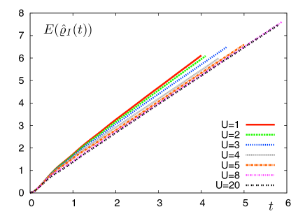
Figure 20: Von-Neumann entropy of the bisected half-chain between sites $\{1,\dots,16\}$ and $\{17,\dots,32\}$ vs. time for various interaction strengths $U$.

X Relationship to kinematical approaches

We only very briefly touch this issue here. In this work, similarly to Refs. Relax ; Tegmark ; Barthel , we have considered local relaxation to an apparent equilibrium state. The overall system undergoes time evolution under a local Hamiltonian $\hat{H}$, whereas subsystems $I$ appear relaxed. This observation is in an interesting relationship to kinematical approaches Jaynes ; Page ; Page2 ; Kine1 . Indeed, if one draws a random pure state of a large system, this will be—in the limit of a large environment—almost always maximally mixed. Random here means, drawn from the unitarily invariant measure, so the Haar measure Page ; Page2 ; Kine1 ; Kine2 (or a measure on the energy shell for Gaussian states Kine3 ). So one could argue that “most states are locally relaxed”. This might render a relaxation to high entropy states plausible. Yet, ironically, the image of the positive time axis under the time evolution corresponds, of course, to a one-dimensional manifold in state space: So in order to show that relaxation follows from such a kinematical argument, one has to demonstrate that for a given local Hamiltonian, time evolution ensures that the state of the global system stays within the typical subspace. This is an interesting programme and the proof constitutes an interesting challenge in case of interacting systems, which has not yet been completed. In case of free systems as in Ref. Relax , the findings may indeed be interpreted in this way.

XI Summary

In this work, we have introduced a setting in which local relaxation in quantum many-body systems can be probed, without the need of actually addressing single sites: This is the setting of a Bose-Hubbard model, in which preparation and read-out can be done with period-$2$ translational invariance, as can be achieved by exploiting optical superlattices. We have approached this idea by deriving analytical expressions for the relevant quantities in case of the free limits of $U=0$ and $U=\infty$ in the Bose-Hubbard model, as well as using a systematic t-DMRG approach in the time-dependent interacting case. For the $U=0$ case, we presented in detail a true convergence of subsystems to the maximum entropy state in $1$-norm. In several ways, the interacting setting reminded of the non-interacting case, certainly concerning the mechanism of relaxation. The time-scales are different, however, showing a faster relaxation compared to the inverse square-root dependence. Also, the dependence on the interaction strength reflects the same dependence in the corresponding Gibbs state of the Hamiltonian the system is quenched to.

In this way, signatures of local relaxation can be measured with present technology: Local densities are found to relax to those of a quasi-thermal state on well-defined time scales, often with a similar to inverse square-root time dependence. More sophisticated measurements would reveal correlators and density-density correlations, again showing local relaxation in a characteristic fashion. Hence, by exploiting period-$2$ translational invariance, one has a tool at hand that effectively can be viewed as if one looked at a small local subsystem, showing all signatures of the local relaxation. In turn, the quasi-momentum distribution is a global quantity, one that shows in the free limit of $U=0$ no relaxation at all, and merely detects the boundary conditions quickly.

Hence, this is a quite exciting situation that both the presence of the memory of the initial condition could be experimentally probed—in the absence of relaxation in “too global quantities”—as well as local relaxation: Locally, the system “appears relaxed”, for very long times, until recurrences become relevant. The technology offered by recent advances in the use of optical superlattices should hence open up the way to experimentally access such fundamental and old questions as the mechanism of local relaxation in quantum many-body systems.

XII Acknowledgements

We would like to thank T. Barthel, P. Calabrese, R. Fazio, M.B. Hastings, C. Kollath, T.J. Osborne, B. Paredes, and M.M. Wolf for discussions related to the subject of local relaxation in quenched quantum many-body systems. We specifically thank I. Bloch for several fruitful discussions on non-equilibrium dynamics and optical superlattices, and for the kind hospitality in Mainz. This work has been supported by the EU (QAP, COMPAS), the DFG (FOR 801), the EPSRC, the EURYI, and Microsoft Research.

XIII Appendix: Proofs

We largely follow Ref. Relax to show local relaxation. For the special situation at hand—one spatial dimension and $|\psi(0)\rangle=|1,0,\dots,1,0\rangle$— the proofs simplify significantly and we state them here for completeness.

XIII.1 Preliminaries

The bosonic operators evolve in time according to (this can be shown by solving Heisenberg’s equation of motion or applying the Baker-Hausdorff formula)

$$\hat{b}_{i}(t)=\mathrm{e}^{\mathrm{i}t\hat{H}}\hat{b}_{i}\mathrm{e}^{-\mathrm{i}t\hat{H}}=\sum_{j=1}^{L}V_{i,j}\hat{b}_{j},\;\;V(L,t)=\mathrm{e}^{-\mathrm{i}tH},$$ (49)

where the entries of the Hamilton matrix $H$ are given by $H_{i,j}=-\delta_{\text{dist}(i,j),1}$. For the translationally invariant setting one has

$$V_{i,j}(L,t)=\frac{1}{L}\sum_{k=1}^{L}\mathrm{e}^{-\mathrm{i}t\lambda_{k}}\mathrm{e}^{2\pi\mathrm{i}k(i-j)/L},$$ (50)

where

$$\lambda_{k}=-2\cos(2\pi k/L)$$ (51)

are the eigenvalues of $V$.

XIII.2 Proof of local relaxation

In this subsection, we rigorously show that for large times and large system size, the state of a subblock $I$ becomes exactly a maximum entropy state. The key ingredients to this proof are Lieb-Robinson ideas and a central limit-type theorem. The proof is not too technically involved, but also far from being trivial, and we present it for completeness. It is, after all, quite astonishing that one does arrive at maximum entropy states without a time average. This proof largely follows Ref. Relax , adapted to our situation of an alternating sequence of bosons and no bosons per site as initial condition.

We can now no longer merely think in terms of moments, as we want to prove convergence of the state itself. Instead of studying the quantum state, we investigate its characteristic function in phase space. Pointwise convergence of the characteristic function implies convergence in trace norm for the state. For subsets $I\subset\mathcal{L}=\{1,\dots,L\}$, the local state on $I$ is given by a partial trace

$$\hat{\varrho}_{I}(L,t)=\text{tr}_{\mathcal{L}\backslash I}\bigl{[}|\psi(t)\rangle\langle\psi(t)|\bigr{]},$$ (52)

and the corresponding characteristic function to represent the state $\hat{\varrho}_{I}$ is defined as

$$\chi(\boldsymbol{\alpha};t)=\text{tr}\Bigl{[}\hat{\varrho}_{I}\prod_{i\in I}\hat{D}_{i}(\alpha_{i})\Bigr{]},\;\hat{D}_{i}=\mathrm{e}^{\alpha_{i}\hat{b}_{i}^{\dagger}-\alpha_{i}^{*}\hat{b}_{i}}.$$ (53)

Here the $\alpha_{i}\in\mathbb{C}$ are the complex phase space coordinates and

$$|\psi(t)\rangle=\mathrm{e}^{-\mathrm{i}t\hat{H}}|1,0\dots,1,0\rangle$$ (54)

is the time evolved state vector. We aim at showing that the state of any subblock $I=\{1,\dots,s\}$ of $s$ consecutive sites locally relaxes. For any such block, we find from Eq. (49) that

$$\chi=\langle 1,0,\dots,1,0|\prod_{i\in\mathcal{L}}\hat{D}_{i}(\beta_{i})|1,0,\dots,1,0\rangle,$$ (55)

where we defined

$$\beta_{i}(t)=\sum_{j=1}^{s}\alpha_{j}V_{j,i}^{*}(t).$$ (56)

We thus find the following explicit form of the characteristic function of $\hat{\varrho}_{I}(L,t)$:

$$\begin{split}\chi&=\prod_{i=1}^{L/2}\langle 0|\hat{D}_{2i}(\beta_{2i})|0\rangle\prod_{i=1}^{L/2}\langle 1|\hat{D}_{2i-1}(\beta_{2i-1})|1\rangle\\ &=\mathrm{e}^{-\boldsymbol{\beta}^{\dagger}\boldsymbol{\beta}/2}\prod_{i=1}^{L/2}(1-|\beta_{2i-1}|^{2}),\end{split}$$ (57)

where we made use of the explicit matrix elements of the displacement operator in the Fock basis. Now, $\boldsymbol{\beta}^{\dagger}\boldsymbol{\beta}=\boldsymbol{\alpha}^{\dagger}\boldsymbol{\alpha}$ follows from unitarity of $V$ and we proceed by proving that the above product converges pointwise in $\boldsymbol{\alpha}$ to $\exp(-\boldsymbol{\alpha}^{\dagger}\boldsymbol{\alpha}/2)$.

XIII.2.1 The causal cone

The key ingredient for most of what follows is the fact that the entries $V_{i,j}=V_{i-j}$ become arbitrarily small for sufficiently large $L$ and $t$. This can be seen as follows: The $V_{i,j}=V_{i-j}$ may be thought of as Riemann-sum approximation to the integral

$$\frac{1}{2\pi}\int_{0}^{2\pi}\mathrm{d}\phi\,\mathrm{e}^{2\mathrm{i}Jt\cos(\phi)}\mathrm{e}^{\mathrm{i}l\phi}=\mathrm{i}^{l}J_{l}(2Jt),$$ (58)

where $J_{l}$ is a Bessel function of the first kind, for which one has $J_{l}(x)\leq x^{-1/3}$ for all $x\geq 0$ and all $l$. The error involved in this approximation is

$$\left|V_{l}-\mathrm{i}^{l}J_{l}(2Jt)\right|\leq\frac{\pi(l+2Jt)}{L},$$ (59)

i.e., we have the bound

$$\left|V_{l}\right|\leq\frac{\pi(l+2Jt)}{L}+(2Jt)^{-1/3},$$ (60)

which converges to zero if we fix $l$, let $L\rightarrow\infty$ and then $t\rightarrow\infty$. However, we need a bound on the entries of $V$ for all $l$. To this end we complement the above bound with a Lieb-Robinson type bound on the influence of sites with large $l$: As $H_{i,j}=0$ for $\text{dist}(i,j)>1$, we have $(H^{n})_{i,j}=0$ for $n<\text{dist}(i,j)=:d$, i.e.,

$$V_{i,j}=\sum_{n\geq d}\frac{(\mathrm{i}t)^{n}}{n!}\left(H^{n}\right)_{i,j}.$$ (61)

Now, for any matrix $M$ one has $|M_{i,j}|\leq\|M\|$, where $\|\cdot\|$ indicates the operator norm. Furthermore, $n!\geq(n/3)^{n}$. We thus find

$$\left|V_{i,j}\right|\leq\sum_{n\geq d}\frac{\left(6Jt\right)^{n}}{n^{n}}\leq\sum_{n\geq d}\frac{\left(6Jt\right)^{n}}{d^{n}}=\frac{(6Jt/d)^{d}}{1-6Jt/d},$$ (62)

independent of $L$. Hence, matrix entries $V_{i,j}$ with $\text{dist}(i,j)>6Jt$ are exponentially suppressed in $\text{dist}(i,j)$, defining a ”causal cone” as the influence of sites with $\text{dist}(i,j)>6Jt$ is exponentially small in $\text{dist}(i,j)$. For given $\varepsilon>0$ we have $|V_{i,j}|<\varepsilon$ if $\text{dist}(i,j)>B(t)$, where $B(t)$ is given by the solution to $(6Jt/B(t))^{B(t)}=\varepsilon(1-6Jt/B(t))$. A crude bound on $B(t)$ may be obtained from noting that

$$\frac{(6Jt/d)^{d}}{1-6Jt/d}\leq\frac{6Jt/d}{1-6Jt/d}.$$ (63)

Combining this with the bound for $i,j$ inside the cone from above, we find for given $\varepsilon>0$ and all $i,j$ that

$$|V_{i,j}|<\varepsilon\text{ for all }t:\frac{4}{\varepsilon^{2}}<Jt<\frac{L}{4\pi^{2}}\frac{\varepsilon^{2}}{8\varepsilon+6}.$$ (64)

The entries of $V$ are thus arbitrarily small for sufficiently large $L$ and $t$. In particular $\lim_{t\rightarrow\infty}\lim_{L\rightarrow\infty}|V_{i,j}|=0$.

XIII.2.2 Central limit-type argument

We have from the previous section that $|V_{i,j}|$ becomes arbitrarily small for sufficiently $L$ and $t$. Thus, for given $\boldsymbol{\alpha}$ the $|\beta_{i}|\leq\sum_{j=1}^{s}|\alpha_{j}||V_{j,i}|$ become arbitrarily small, in particular we may assume $|\beta_{i}|<1/2$. Now, for $|x|<1/2$ one has $|\log(1+x)-x|\leq x^{2}$, i.e.,

$$\begin{split}\sum_{i=1}^{L/2}\left|\log(1-|\beta_{2i-1}|^{2})+|\beta_{2i-1}|^{2}\right|\leq\sum_{i=1}^{L/2}|\beta_{2i-1}|^{4}\\ \leq\sup_{j}|\beta_{j}|^{2}\sum_{i=1}^{L/2}|\beta_{2i-1}|^{2}.\end{split}$$ (65)

Now,

$$\sum_{i=1}^{L/2}|\beta_{2i-1}|^{2}=\sum_{k,l=1}^{s}\alpha_{k}^{*}\alpha_{l}\sum_{i=1}^{L/2}V_{k,2i-1}V_{l,2i-1}^{*},$$ (66)

where, using Eq. (50),

$$\begin{split}\sum_{i=1}^{L/2}V_{k,2i-1}V_{l,2i-1}^{*}=\frac{1}{L^{2}}\sum_{r,s=1}^{L}\mathrm{e}^{\mathrm{i}t(\lambda_{s}-\lambda_{r})}\mathrm{e}^{\frac{2\pi}{L}\mathrm{i}(r(k+1)-s(l+1))}\\ \times\sum_{i=1}^{L/2}\mathrm{e}^{\frac{4\pi}{L}\mathrm{i}i(s-r)},\end{split}$$ (67)

where we find for the last line

$$\begin{split}\frac{2}{L}\sum_{i=1}^{L/2}\mathrm{e}^{2\pi\mathrm{i}i(s-r)/(L/2)}=\delta_{s,r}+\delta_{s-r,L/2}+\delta_{r-s,L/2},\end{split}$$ (68)

i.e.,

$$\begin{split}\sum_{i=1}^{L/2}V_{k,2i-1}^{*}V_{l,2i-1}&=\frac{1}{2}\delta_{k,l}\hskip 85.35826pt\\ &\;\;\;\;-\frac{(-1)^{l}}{2L}\sum_{r=1}^{L}\mathrm{e}^{4J\mathrm{i}t\cos(2\pi r/L)}\mathrm{e}^{\frac{2\pi}{L}\mathrm{i}r(k-l)}\\ &=\frac{1}{2}\delta_{k,l}-\frac{(-1)^{l}}{2}V_{k,l}(2t).\end{split}$$ (69)

Thus,

$$\begin{split}\Bigl{|}\sum_{i=1}^{L/2}|\beta_{2i}|^{2}-\frac{\boldsymbol{\alpha}^{\dagger}\boldsymbol{\alpha}}{2}\Bigr{|}\leq\sum_{i,j=1}^{s}|\alpha_{k}||\alpha_{l}|V_{k,l}(2t)|,\end{split}$$ (70)

which converges to zero for large $L$ and $t$. We thus arrive at the desired statement:

$$\lim_{t\rightarrow\infty}\lim_{L\rightarrow\infty}\chi(\boldsymbol{\alpha};L,t)=\mathrm{e}^{-\boldsymbol{\alpha}^{\dagger}\boldsymbol{\alpha}}$$ (71)

pointwise in $\boldsymbol{\alpha}$.

XIII.3 Correlations after a sudden quench ($\mathbf{U=0}$)

In this section, we give explicit forms for the two-point correlations,

$$f_{i,j}=\langle\hat{b}_{i}^{\dagger}(t)\hat{b}_{j}(t)\rangle,$$ (72)

and density-density correlations,

$$g_{i,j}=\langle\hat{n}_{i}(t)\hat{n}_{j}(t)\rangle,$$ (73)

for the translationally invariant non-interacting case, $U=0$. We already know the asymptotic behavior from the previous section (for long times, neighboring sites become uncorrelated as the state converges to a direct product of Gaussians) but the goal here is to derive explicit expressions for all times.

We find from Eqs. (49,50) that

$$\begin{split}f_{i,j}&=\frac{1}{L}\sum_{p,q=1}^{L}\mathrm{e}^{\mathrm{i}t(\lambda_{q}-\lambda_{p})}\mathrm{e}^{2\pi\mathrm{i}(pj-qi)/L}\\ &\hskip 56.9055pt\times\frac{1}{L}\sum_{k=1}^{L/2}\mathrm{e}^{2\pi\mathrm{i}(2k-1)(q-p)/L},\end{split}$$ (74)

where the term in the last line evaluates to

$$\begin{split}\frac{\mathrm{e}^{-2\pi\mathrm{i}(q-p)/L}}{L}\sum_{k=1}^{L/2}\mathrm{e}^{2\pi\mathrm{i}k(q-p)/(L/2)}\hskip 56.9055pt\\ =\frac{1}{2}\left(\delta_{p,q}-\delta_{q-p,L/2}-\delta_{p-q,L/2}\right).\end{split}$$ (75)

We thus have

$$\begin{split}f_{i,j}=\frac{1}{2}\delta_{i,j}-\frac{(-1)^{i}}{2L}\sum_{p=1}^{L}\mathrm{e}^{4J\mathrm{i}t\cos(2\pi p/L)}\mathrm{e}^{2\pi\mathrm{i}p(j-i)/L},\end{split}$$ (76)

which yields a particularly simple form in the thermodynamic limit $L\rightarrow\infty$

$$f_{i,j}\rightarrow\frac{1}{2}\delta_{i,j}-\frac{(-1)^{i}\mathrm{i}^{j-i}}{2}J_{j-i}(4Jt),$$ (77)

where $J_{n}$ is a Bessel function of the first kind. Thus, the total number of particles at even sites

$$\sum_{i\text{ even}}\left\langle\hat{n}_{i}(t)\right\rangle=\frac{L}{4}-\frac{L}{4}J_{0}(4Jt)$$ (78)

is a truly local quantity in this translationally invariant setting.

The above allows us to derive the quasi-momentum distribution,

$$\begin{split}S(q,t)&=\frac{1}{L}\sum_{i,j}\mathrm{e}^{\mathrm{i}q(i-j)}f_{i,j}\\ &=\frac{1}{2}-\frac{1}{2L^{2}}\sum_{p=1}^{L}\mathrm{e}^{4J\mathrm{i}t\cos(2\pi p/L)}\\ &\;\;\;\;\;\;\times\sum_{i,j=1}^{L}\mathrm{e}^{\mathrm{i}i(q+\pi-2\pi p/L)}\mathrm{e}^{\mathrm{i}j(2\pi p/L-q)},\end{split}$$ (79)

where the last term vanishes for $Lq/(2\pi)\in\{1,\dots,L\}$, yielding $S(q,t)=1/2$. For all other $q\in[0,2\pi]$ we find

$$S(q,t)=\frac{1}{2}+\frac{\mathrm{i}}{L^{2}}\sum_{p=1}^{L}\mathrm{e}^{4J\mathrm{i}t\cos(2\pi p/L)}\frac{\sin^{2}(Lq/2)}{\sin(2\pi p/L-q)}.$$ (80)

To derive the density-density correlations, we first observe that for

$$h_{k,l,r,s}=\langle n_{1},n_{2},\dots,n_{L}|\hat{b}^{\dagger}_{k}\hat{b}_{l}\hat{b}^{\dagger}_{r}\hat{b}_{s}|n_{1},n_{2},\dots,n_{L}\rangle,$$ (81)

we have (writing $\delta_{k\neq l}=1-\delta_{k,l}$)

$$\begin{split}h_{k,l,r,s}&=\left(\delta_{k,l}+\delta_{k\neq l}\right)\left(\delta_{r,s}+\delta_{r\neq s}\right)h_{k,l,r,s}\\ &=\delta_{k,l}\delta_{r,s}n_{k}n_{r}+\delta_{k\neq l}\delta_{r\neq s}h_{k,l,r,s}\\ &=\delta_{k,l}\delta_{r,s}n_{k}n_{r}+\delta_{k\neq l}\delta_{k,s}\delta_{l,r}n_{k}(1+n_{l}).\end{split}$$ (82)

Thus,

$$\begin{split}g_{i,j}=&\sum_{k=1}^{L/2}V_{i,2k-1}^{*}V_{i,2k-1}\sum_{r=1}^{L/2}V_{j,2r-1}^{*}V_{j,2r-1}\\ &+2\sum_{k,l=1}^{L/2}\delta_{k\neq l}V_{i,2k-1}^{*}V_{i,2l-1}V_{j,2l-1}^{*}V_{j,2k-1},\end{split}$$ (83)

and therefore,

$$\begin{split}g_{i,j}=&f_{i,i}f_{j,j}+f_{i,j}(\delta_{i,j}+f_{j,i})\\ &-2\sum_{k=1}^{L/2}|V_{i,2k-1}|^{2}|V_{j,2k-1}|^{2}.\end{split}$$ (84)

This expression yields

$$\begin{split}&\langle\hat{N}_{e}(t)\hat{N}_{o}(t)\rangle-\langle\hat{N}_{e}(t)\rangle\langle\hat{N}_{o}(t)\rangle\\ =&\sum_{i,j=1}^{L/2}\left(g_{2i,2j-1}-f_{2i,2i}f_{2j-1,2j-1}\right)\\ =&\sum_{i,j=1}^{L/2}f_{2i,2j-1}f_{2j-1,2i}\\ &-2\sum_{k=1}^{L/2}\sum_{i,j=1}^{L/2}|V_{2i,2k-1}|^{2}|V_{2j-1,2k-1}|^{2},\end{split}$$ (85)

where, using the unitarity of $V$,

$$\begin{split}&\sum_{i,j=1}^{L/2}|V_{2i,2k-1}|^{2}|V_{2j-1,2k-1}|^{2}\\ &=\left(1-\sum_{i=1}^{L/2}|V_{2i-1,2k-1}|^{2}\right)\sum_{j=1}^{L/2}|V_{2j-1,2k-1}|^{2}\\ &=(1-f_{2k-1,2k-1})f_{2k-1,2k-1},\end{split}$$ (86)

and, using the explicit form of $f_{i,j}$ and identifying Kronecker deltas,

$$\begin{split}&\sum_{i,j=1}^{L/2}f_{2i,2j-1}f_{2j-1,2i}\\ &=-\frac{1}{16}\sum_{\begin{subarray}{c}p,q=1\\ \frac{p+q}{L/2}\in{\mathbbm{Z}}\end{subarray}}^{L}\mathrm{e}^{4J\mathrm{i}t(\cos(2\pi p/L)+\cos(2\pi q/L))-2\pi\mathrm{i}(p-q)/L}\\ &=-\frac{1}{16}\sum_{p=1}^{L}\mathrm{e}^{8J\mathrm{i}t\cos(2\pi p/L)}+\frac{L}{16}.\end{split}$$ (87)

For large $L$ we then find

$$\begin{split}&\langle\hat{N}_{e}(t)\hat{N}_{o}(t)\rangle-\langle\hat{N}_{e}(t)\rangle\langle\hat{N}_{o}(t)\rangle\\ &\hskip 11.38092pt\rightarrow-\frac{L}{16}\left(3+J_{0}(8Jt)-4[J_{0}(4Jt)]^{2}\right).\end{split}$$ (88)

XIII.4 Correlations after a sudden quench ($\mathbf{U\rightarrow\infty}$)

Using the results for $U=0$ (XIII.3) we can now easily derive analytical expressions for local densities

$$f_{i,i}=\langle\hat{n}_{i}(t)\rangle,$$ (89)

next-neighbour two-point correlations

$$f_{i+1,i}=\langle\hat{b}^{\dagger}_{i+1}(t)\hat{b}_{i}(t)\rangle$$ (90)

and density-density correlations

$$g_{i,j}=\langle\hat{n}_{i}(t)\hat{n}_{j}(t)\rangle$$ (91)

for $U\rightarrow\infty$. For simplicity we assume even particle numbers $N=L/2$. With Eqs. (22), (23) it follows that Eqs. (89)-(91) are also valid for after the mapping to fermions, with the bosonic creation- and annihilation operators replaced by fermionic ones. Because of the identical time evolution of the bosonic- and fermionic operators (equation (12) respectively (25)) we find essentially the same results for the local densities and the next-neighbour two-point correlations like in section XIII.3 as we did not make any use of commutation relations in the derivation of the bosonic respectively fermionic results:

$$f_{i,i} = \frac{1}{2}-\frac{(-1)^{i}}{2L}\sum_{p=1}^{L}\mathrm{e}^{4J\mathrm{i}t\cos(2\pi p/L)},$$ (92)

$$f_{i+1,i} = -\frac{(-1)^{i+1}}{2L}\sum_{p=1}^{L}\mathrm{e}^{4J\mathrm{i}t\cos(2\pi p/L)}\mathrm{e}^{-2\pi\mathrm{i}p/L}.$$ (93)

In contrast to this, the results for the density-density correlations differ. For fermionic operators a similar derivation to Eq. (82) yields

$$\begin{split}\tilde{h}_{k,l,r,s}=&\langle n_{1},n_{2},\dots,n_{L}\lvert\hat{c}^{\dagger}_{k}\hat{c}_{l}\hat{c}^{\dagger}_{r}\hat{c}_{s}\rvert n_{1},n_{2},\dots,n_{L}\rangle\\ =&\delta_{k,l}\delta_{r,s}n_{k}n_{r}+\delta_{k\neq l}\delta_{k,s}\delta_{l,r}n_{k}(1-n_{l}).\end{split}$$ (94)

This finally leads to

$$\begin{split}g_{i,j}=\tilde{f}_{i,i}\tilde{f}_{j,j}+\tilde{f}_{i,j}(\delta_{i,j}-\tilde{f}_{j,i})\end{split}$$ (95)

with $\tilde{f}_{i,j}=\langle\hat{c}^{\dagger}_{i}(t)\hat{c}_{j}(t)\rangle$. Using the explicit form of the time-evolved operators in Eqs. (12), (25) and the absence of any signs resulting from commutation relations it is easy to see that $\tilde{f}_{i,j}$ is identical with $f_{i,j}$ for free bosons (see XIII.3). This finally leads to Eq. (26). Using the results of XIII.3, the global density-density correlator is then given by

$$\begin{split}&\langle\hat{N}_{e}(t)\hat{N}_{o}(t)\rangle-\langle\hat{N}_{e}(t)\rangle\langle\hat{N}_{o}(t)\rangle\\ &=-\sum_{i,j=1}^{L/2}f_{2i,2j-1}f_{2j-1,2i}\\ &=\frac{L}{16}\left(\frac{1}{L}\sum_{p=1}^{L}\mathrm{e}^{8J\mathrm{i}t\cos(2\pi p/L)}-1\right).\end{split}$$ (96)

For large $L$ this yields

$$\begin{split}&\langle\hat{N}_{e}(t)\hat{N}_{o}(t)\rangle-\langle\hat{N}_{e}(t)\rangle\langle\hat{N}_{o}(t)\rangle\\ &\rightarrow-\frac{L}{16}\left(1-J_{0}(8Jt)\right).\end{split}$$ (97)

References

- (1) B.M. McCoy and E. Barouch, Phys. Rev. A 3, 786 (1971).
- (2) C. Kollath, A. Läuchli, and E. Altman, Phys. Rev. Lett. 98, 180601 (2007).
- (3) M. Cramer, C.M. Dawson, J. Eisert, and T.J. Osborne, Phys. Rev. Lett. 100, 030602 (2008).
- (4) M. Cramer, A. Flesch, I.A. McCulloch, U. Schollwöck, and J. Eisert, Phys. Rev. Lett. 101, 063001 (2008).
- (5) M. Tegmark and L. Yeh, Physica A, 202, 342 (1994).
- (6) T. Barthel and U. Schollwöck, Phys. Rev. Lett. 100, 100601 (2008).
- (7) J. Eisert, M.B. Plenio, J. Hartley, and S. Bose, Phys. Rev. Lett. 93, 190402 (2004).
- (8) M.B. Plenio, J. Hartley, and J. Eisert, New J. Phys. 6, 36 (2004).
- (9) K. Sengupta, S. Powell, and S. Sachdev, Phys. Rev. A 69, 053616 (2004).
- (10) M.J. Hartmann, G. Mahler, and O. Hess, Phys. Rev. E 70, 066148 (2004).
- (11) S.D. Huber, E. Altman, H.P. Büchler, and G. Blatter, Phys. Rev. B 75, 085106 (2007).
- (12) V. Eisler and I. Peschel, J. Stat. Mech. (2007) P06005.
- (13) M.B. Hastings, Phys. Rev. B 77, 144302 (2008).
- (14) M.B. Hastings and L.S. Levitov, arXiv:0806.4283.
- (15) P. Calabrese and J. Cardy, Phys. Rev. Lett. 96, 136801 (2006).
- (16) P. Calabrese and J. Cardy, J. Stat. Mech. (2007) P10004.
- (17) W.H. Zurek, U. Dorner, and P. Zoller, Phys. Rev. Lett. 95, 105701 (2005).
- (18) M. Rigol, V. Dunjko, V. Yurovsky, and M. Olshanii, Phys. Rev. Lett. 98, 050405 (2007).
- (19) M. Rigol, A. Muramatsu, and M. Olshanii, Phys. Rev. A 74, 053616 (2006).
- (20) K. Rodriguez, S.R. Manmana, M. Rigol, R.M. Noack and A. Muramatsu, New J. Phys. 8, 169 (2006).
- (21) P. Calabrese and J. Cardy, J. Stat. Mech. (2005) P04010.
- (22) J. Eisert and T.J. Osborne, Phys. Rev. Lett. 97, 150404 (2006).
- (23) S. Bravyi, M.B. Hastings, and F. Verstraete, Phys. Rev. Lett. 97, 050401 (2006).
- (24) G. De Chiara, S. Montangero, P. Calabrese, and R. Fazio, J. Stat. Mech. (2006) P03001.
- (25) A. Laeuchli and C. Kollath, J. Stat. Mech. (2008) P05018.
- (26) S. R. Manmana, S. Wessel, R. M. Noack, and A. Muramatsu, Phys. Rev. Lett. 98, 210405 (2007).
- (27) M. A. Cazalilla, Phys. Rev. Lett. 97, 156403 (2006).
- (28) M. Eckstein and M. Kollar, Phys. Rev. Lett. 100, 120404 (2008).
- (29) P. Barmettler, A.M. Rey, E.A. Demler, M.D. Lukin, I. Bloch, and V. Gritsev, Phys. Rev. A 78, 012330 (2008).
- (30) M. Möckel and S. Kehrein, Phys. Rev. Lett. 100, 175702 (2008).
- (31) T. Dudnikova, A. Komech, and H. Spohn, J. Math. Phys. 44, 2596 (2003).
- (32) M.J. Hartmann and M.B. Plenio, Phys. Rev. Lett. 100, 070602 (2008).
- (33) N. Schuch, M.M. Wolf, K.G.H. Vollbrecht, and J.I. Cirac, New J. Phys. 10, 033032 (2008).
- (34) D.C. Roberts and K. Burnett, Phys. Rev. Lett. 90, 150401 (2003).
- (35) U.R. Fischer, R. Schützhold, and M. Uhlmann, Phys. Rev. A 77, 043615 (2008).
- (36) A. Sen De, U. Sen, and M. Lewenstein, Phys. Rev. A 72, 052319 (2005).
- (37) E.T. Jaynes, Phys. Rev. 106, 620 (1957).
- (38) Similar statements may also be true in momentum space for some observables, and in fact, using an approximate Wegner flow method, such a relaxation has been identified in interacting systems Moeckel .
- (39) Such bounds to the speed of information transfer have rigorously been shown for finite-dimensional systems such as spins or fermions LR ; Hastings ; LRReview , and for free bosonic systems Nachtergaele ; HarmonicLiebRobinson ; Buer .
- (40) E.H. Lieb and D.W. Robinson, Commun. Math. Phys. 28, 251 (1972).
- (41) M.B. Hastings and T. Koma, Commun. Math. Phys. 265, 781 (2006).
- (42) B. Nachtergaele and R. Sims, arXiv:0712.3318.
- (43) M. Cramer, A. Serafini, and J. Eisert, arXiv:0803.0890.
- (44) B. Nachtergaele, H. Raz, B. Schlein, and R. Sims, Commun. Math. Phys. 286, 1073 (2009).
- (45) O. Buerschaper, M.M. Wolf, and J.I. Cirac, in preparation (2008).
- (46) Note that for long-range correlation functions, results from conformal field theory also strongly suggest a relaxation in the asymptotic behavior when quenched to critical quantum systems Calabrese ; CalabreseLong .
- (47) D.N. Page, Phys. Rev. Lett. 71, 1291 (1993).
- (48) S.K. Foong and S. Kanno, Phys. Rev. Lett. 72, 1148 (1994).
- (49) S. Popescu, A.J. Short, and A. Winter, Nature Physics 2, 754 (2006).
- (50) D. Gross, K. Audenaert, and J. Eisert, J. Math. Phys. 48, 052104 (2007).
- (51) A. Serafini, O.C.O. Dahlsten, D. Gross, and M.B. Plenio, J. Phys. A 40, 9551 (2007).
- (52) M. Greiner, O. Mandel, T. W. Hänsch, and I. Bloch, Nature 419, 51 (2002).
- (53) A.K. Tuchman, C. Orzel, A. Polkovnikov, and M.A. Kasevich, cond-mat/0504762.
- (54) T. Kinoshita, T. Wenger, and D.S. Weiss, Nature 440, 900 (2006).
- (55) L.E. Sadler, J.M. Higbie, S.R. Leslie, M. Vengalattore, and D.M. Stamper-Kurn, Nature 443, 312 (2006).
- (56) S. Hofferberth, I. Lesanovsky, B. Fischer, T. Schumm, and J. Schmiedmayer, Nature 449, 324 (2007).
- (57) S. Fölling, S. Trotzky, P. Cheinet, M. Feld, R. Saers, A. Widera, T. Mueller, and I. Bloch, Nature 448, 1029 (2007).
- (58) S. Trotzky, P. Cheinet, S. Fölling, M. Feld, U. Schnorrberger, A.M. Rey, A. Polkovnikov, E.A. Demler, M.D. Lukin, and I. Bloch, Science 319 5861 (2008).
- (59) A.M. Rey, V. Gritsev, I. Bloch, E. S. Hofferberth, I. Lesanovsky, B. Fischer, T. Schumm, and J. Schmiedmayer, Nature 449, 324 (2007).
- (60) B. Vaucher, S.R. Clark, U. Dorner, and D. Jaksch, New J. Phys. 9, 221 (2007).
- (61) E. Altman, E.A. Demler, and M.D. Lukin, Phys. Rev. A 70, 013603 (2004).
- (62) S.R. White, Phys. Rev. Lett. 69, 2863 (1992).
- (63) U. Schollwöck, Rev. Mod. Phys. 77, 259 (2005).
- (64) G. Vidal, Phys. Rev. Lett. 93, 040502 (2004).
- (65) A.J. Daley, C. Kollath, U. Schollwöck, and G. Vidal, J. Stat. Mech. (2004) P04005.
- (66) S. R. White and A. Feiguin, Phys. Rev. Lett. 93, 076401 (2004).
- (67) C. Kollath, U. Schollwöck, J. von Delft and W. Zwerger, Phys. Rev. A 71, 053606 (2005).