ROTATION AND SURFACE ABUNDANCE PECULIARITIES
IN A-TYPE STARS

Abstract

In an attempt of clarifying the connection between the photospheric abundance anomalies and the stellar rotation as well as of exploring the nature of “normal A” stars, the abundances of seven elements (C, O, Si, Ca, Ti, Fe, and Ba) and the projected rotational velocity for 46 A-type field stars were determined by applying the spectrum-fitting method to the high-dispersion spectral data obtained with BOES at BOAO. We found that the peculiarities (underabundances of C, O, and Ca; an overabundance of Ba) seen in slow rotators efficiently decrease with an increase of rotation, which almost disappear at $v_{\rm e}\sin i\mathrel{\hbox{\hbox to0.0pt{\hbox{\lower 4.0pt\hbox{$\sim$}}\hss}\hbox{$>$}}}100$ km s^-1. This further suggests that stars with sufficiently large rotational velocity may retain the original composition at the surface without being altered. Considering the subsolar tendency (by several tenths dex below) exhibited by the elemental abundances of such rapidly-rotating (supposedly normal) A stars, we suspect that the gas metallicity may have decreased since our Sun was born, contrary to the common picture of galactic chemical evolution.

I INTRODUCTION

Since unevolved A-type stars on (or near to) the upper main-sequence have masses around $\sim 2M_{\odot}$, their surface abundances may retain information of the composition of the past galactic gas ($\mathrel{\hbox{\hbox to0.0pt{\hbox{\lower 4.0pt\hbox{$\sim$}}\hss}\hbox{$<$}}}10^{9}$ yr ago) from which they formed; this would provide us with an important opportunity to investigate the “recent” chemical evolution history of the Galaxy. However, such a study using A stars as a probe of late-time history of chemical evolution has rarely been done in spite of its potential significance in contrast to the case of old-time history where a number of researches (using longer-lived F–G–K dwarfs) are available. This is related to the fact that a large fraction of them are rapid rotators (typically $v_{\rm e}\sin i\sim$ 100–200 km s^-1 on the average; see, e.g., Royer et al. 2002a, b) whose spectra are technically difficult to analyze because lines are broad and smeared out, while sharp-lined slow rotators easy to handle tend to show abundance anomalies (chemically peculiar stars or CP stars). As a matter of fact, most spectroscopic analyses of A stars have focused on sharp-lined ones with $v_{\rm e}\sin i\mathrel{\hbox{\hbox to0.0pt{\hbox{\lower 4.0pt\hbox{$\sim$}}\hss}\hbox{$<$}}}50$ km s^-1. For this reason, nobody could be sure whether the result obtained for star classified as “normal A” really reflects the initial composition free from any peculiarities.

Therefore, in order to make a further step forward, it is requisite to challenge abundance determinations for “unbiased” sample of A-type stars in general (i.e., without sidestepping rapidly rotating ones), which inevitably requires an application of the spectrum synthesis technique, since reliably measuring the equivalent widths of individual spectral lines is almost hopeless for rapid rotators. Admittedly, while such trials of determining abundances from spectra of A dwarfs including broad-lined ones have recently emerged thanks to the improvement in the method of analysis as well as the data quality, their interests are mainly directed to objects of specific types; e.g., Vega-like stars (Dunkin et al. 1997) or $\lambda$ Bootis stars (Andrievsky et al. 2002) or open-cluster stars (Takeda & Sadakane 1997; Varenne & Monier 1999; Gebran et al. 2008; Gebran & Monier 2008; Fossati et al. 2008). Namely, a systematic study attempting to clarify the characteristics of normal field A-type stars in general, especially in terms of their abundance–rotation connection, seems to have been rarely attempted. To our knowledge, only one such study is Lemke’s (1990, 1993) determinations of C and Ba abundances for some 20 rapidly-rotating A stars with $v_{\rm e}\sin i$ up to $\sim$ 200 km s^-1, which however appear to be still insufficient and inconclusive as judged from his adopted method of approach as well as the number of elements studied.

Considering this situation, we decided to revisit this problem in our own manner based on the high-dispersion spectral data of $\sim 50$ A-type stars in a wide range of $v_{\rm e}\sin i$ (0–300 km s^-1) obtained with BOES at BOAO, while applying the automatic spectrum fitting algorithm (Takeda 1995) which efficiently enables determinations of the abundances (for selected six elements of C, O, Si, Ti, Fe, and Ba) even for rapid rotators showing considerably merged spectra. Our ultimate aim is to clarify the following questions of interest:
— (1) Is there any systematic rotation-dependent tendency between slow and rapid rotators in terms of the abundance anomaly? If so, what is the critical value of $v_{\rm e}\sin i$, above which stars may be regarded as normal?
— (2) What would the abundance characteristics of “normal A-type stars” like, which we may consider as retaining the composition of the galactic gas from which they formed?

We will show that reasonable answers to these points are provided from this study (cf. Sect. V).

II OBSERVATIONAL DATA

We selected 46 apparently bright ($V\mathrel{\hbox{\hbox to0.0pt{\hbox{\lower 4.0pt\hbox{$\sim$}}\hss}\hbox{$<$}}}5$ mag) A-type stars (including Am stars) as our targets, which are listed in Table 1. Figure 1 shows the plots of these stars on the theoretical HR diagram, where we can see that their masses are in the range of $1.5M_{\odot}\mathrel{\hbox{\hbox to0.0pt{\hbox{\lower 4.0pt\hbox{$\sim$}}\hss}\hbox{$<$}}}M\mathrel{\hbox{\hbox to0.0pt{\hbox{\lower 4.0pt\hbox{$\sim$}}\hss}\hbox{$<$}}}3M_{\odot}$.

The observations were carried out on 2008 January 14–16 by using BOES (Bohyunsan Observatory Echelle Spectrograph) attached to the 1.8 m reflector at Bohyunsan Optical Astronomy Observatory. Using 2k$\times$4k CCD (pixel size of 15 $\mu$m $\times$ 15 $\mu$m), this echelle spectrograph enabled us to obtain spectra of wide wavelength coverage (from $\sim$ 3700 $\rm\AA$ to $\sim$ 10000 $\rm\AA$) at a time. We used 200$\mu$m fiber corresponding to the resolving power of $R\simeq 45000$. The integrated exposure time for each star was typically $\sim$ 10–20 min on the average.

The reduction of the echelle spectra (bias subtraction, flat fielding, spectrum extraction, wavelength calibration, and continuum normalization) was carried out with the software developed by Kang et al. (2006). For all 46 targets, we could accomplish S/N ratio of $\sim$ 300–500 at the 6150 $\rm\AA$ region (on which we placed the largest weight on abundance determination; cf. Sect. IV).

III ATMOSPHERIC MODELS

The effective temperature ($T_{\rm eff}$) and the surface gravity ($\log g$) of each program star were determined from the colors of Strömgren’s $uvby\beta$ photometric system with the help of the uvbybetanew program (Napiwotzki, Schönberner, & Wenske 1993), which is an updated/combined version of Moon’s (1985) UVBYBETA (for dereddening) and TEFFLOGG (for determining $T_{\rm eff}$ and $\log g$) codes while based on Kurucz’s (1993) ATLAS9 models. The observed color data ($b-y$, $c_{1}$, $m_{1}$, $\beta_{1}$) of each star were taken from the extensive compilation of Hauck & Mermilliod (1980) via the SIMBAD database. The resulting values of $T_{\rm eff}$ and $\log g$ are given in Table 1.

Then, the model atmosphere for each star was constructed by two-dimensionally interpolating Kurucz’s (1993) ATLAS9 model grid in terms of $T_{\rm eff}$ and $\log g$, where we exclusively applied the solar-metallicity models as was done in Takeda & Sadakane (1997) or Takeda et al. (1999).

IV ANALYSIS

(a) Method and Selected Regions

As a numerical tool for extracting information from the spectra, we adopted the multi-parameter fitting technique developed by Takeda (1995), which can simultaneously determine various parameters affecting the spectra; e.g., abundances of elements showing lines of appreciable contributions, the projected rotational velocity, or the microturbulent velocity.

In the present study, we decided to concentrate on three wavelength regions to be analyzed: (1) 6140–6170 $\rm\AA$ region (hereinafter called “6150 region”) including lines of O, Si, Ca, Fe, and Ba; (2) 5375–5390 $\rm\AA$ region (“5380 region”) including lines of C, Ti, and Fe; (3) 7765–7785 $\rm\AA$ region (“7775 region”) including lines of O and Fe.

(b) Microturbulence

One of the important key parameters is the microturbulence ($\xi$), the choice of which can be critical in abundance determinations from strong line features. Although our method of analysis provides us with a possibility of establishing this parameter as demonstrated by Takeda (1995), whether it works successful or not depends upon situations (i.e., not always possible; especially, its difficulty grows as the rotation becomes higher). Besides, we found from experiences that solutions can sometimes converge at inappropriate (or erroneous) $\xi$ values for the cases of rapid rotators or insufficient data quality.

Accordingly, on the supposition that $\xi$ is a function of $T_{\rm eff}$, we decided to find an appropriate analytical formula by combining the solutions of $\xi$ for the successfully determined cases. For this purpose, special preparatory multi-parameter fitting analyses “including $\xi$ as a variable” (in addition to the elemental abundances and the rotational velocity focused in the standard analysis described in Sect. IV-c) were first carried out for the 6150 region and the 7775 region with an intention to derive the $\xi^{\rm fit}$ values (denoted as $\xi^{\rm fit}_{6150}$ and $\xi^{\rm fit}_{7775}$, respectively). It turned out that $\xi^{\rm fit}_{6150}$ and $\xi^{\rm fit}_{7775}$ could be determined for 33 and 13 stars, respectively, out of 46 program stars.

The correlation of $\xi^{\rm fit}_{6150}$ and $\xi^{\rm fit}_{7775}$ for 13 stars in common is displayed in Figure 2a, where we do not recognize any systematic discordance between these two, though the scatter is rather large (the average difference is $\sim 0.1$ km s^-1 with the standard deviation of $\sim 1$ km s^-1). Figure 2b shows these $\xi^{\rm fit}_{6150}$ and $\xi^{\rm fit}_{7775}$ values plotted against $T_{\rm eff}$, where the $\xi$ results derived for F–G–K dwarfs/subgiants are also overplotted for comparison. We can see from this figure that, as $T_{\rm eff}$ becomes higher, $\xi^{\rm fit}$ increases from $\sim 1$ km s^-1 (at $T_{\rm eff}\sim 6000$ K), to its nearly maximum value of $\sim 4(\pm 2)$ km s^-1 (at $T_{\rm eff}\sim 8000$ K) though with a considerably large scatter, followed by a decreasing tendency toward higher $T_{\rm eff}$ of $\sim 10000$ K (where we know $\xi$ is typically $\sim$ 1–2 km s^-1; cf. Sadakane 1990). Hence, we adopt an analytical formula for the standard microturbulence ($\xi^{\rm std}$)

$$\xi^{\rm std}=4.0\exp\{-[\log(T_{\rm eff}/8000)/A]^{2}\}\\$$ (1)

(where $A\equiv[\log(10000/8000)]/\sqrt{\ln 2}$) with probable uncertainties of $\pm 30\%$, which roughly represents (and encompasses) the observed trend as shown in Figure 2b. Note that such $\xi^{\rm std}$ vs. $T_{\rm eff}$ relation we have defined is in reasonable agreement with previous results (see, e.g., Figure 1 in Coupry & Burkhart 1992 or Figure 2 in Gebran & Monier 2007). The $\xi$ values for each of the 46 stars evaluated by Equation (1), which we will use for abundance determinations, are given in Table 1.

(c) Solutions

Now that the model atmosphere and the microturbulence have been assigned to each star, we can go on to evaluations of elemental abundances by way of synthetic spectrum fitting applied to three wavelength regions. All the atomic data (wavelength, excitation potential, oscillator strengths, damping constants) relevant to the analysis were taken from the extensive compilation of Kurucz & Bell (1995), except for $\log gf$(Fe i 7780.552) (cf. the caption of Table 2). The adopted data of important lines are summarized in Table 2. The non-LTE effect was explicitly taken into account only for the O i triplet lines at 7771–5 $\rm\AA$ (for which the non-LTE correction is known to be appreciably large and its inclusion is necessary; see, e.g., Takeda & Sadakane 1997) based on the statistical equilibrium calculation for O i (cf. Takeda 2003); otherwise, we assumed LTE.

Applying our automatic fitting approach, we adjusted the following parameters to accomplish the best fit at each region: $A^{\rm O}_{6150}$, $A^{\rm Si}_{6150}$, $A^{\rm Ca}_{6150}$, $A^{\rm Fe}_{6150}$, $A^{\rm Ba}_{6150}$, and $v_{\rm e}\sin i_{6150}$ (for the 6150 region); $A^{\rm C}_{5380}$, $A^{\rm Ti}_{5380}$, $A^{\rm Fe}_{5380}$, and $v_{\rm e}\sin i_{5380}$ (for the 5380 region); and $A^{\rm O}_{7775}$, $A^{\rm Fe}_{7775}$, and $v_{\rm e}\sin i_{7775}$ (for the 7775 region). In case that abundance solutions for some elements did not converge (especially for rapid rotators), we had to abandon their determinations and fix them at the solar abundances (i.e., abundances used in the model atmosphere) during the iteration procedure and concentrate on the remaining parameters. Figures 3 (6150 region), 4 (5380 region), and 5 (7775 region) show how the theoretical synthetic spectra corresponding to the final solutions fit the observations.

In order to demonstrate the importance (or unimportance) of the choice of microturbulence for each element, we show the abundance differences between the two cases of $\xi^{\rm fit}$ and $\xi^{\rm std}$ in Figures 6a (6150 region) and b (7775 region) by using the abundance results obtained as by-products from the $\xi^{\rm fit}$-determinination mentioned in the previous Sect. IV-b. It can be seen from these figures that the $A$ values are not very sensitive to the choice of $\xi$, except that only $A^{\rm Ba}$ is considerably $\xi$-dependent because the Ba ii line at 6142.9 $\rm\AA$ (on which $A^{\rm Ba}$ essentially relies) is strongly saturated (cf. Figure 3). In the remainder of this paper, we exclusively refer to the abundances derived by using $\xi^{\rm std}$ as the standard abundances to be discussed.

We also estimated the uncertainties in $A^{\rm X}$ by repeating the analysis while perturbing the standard values of the atmospheric parameters ($T_{\rm eff}^{\rm std}$, $\log g^{\rm std}$, $\xi^{\rm std}$) interchangeably by $\pm 300$ K , $\pm 0.3$ dex, and $\pm 0.3\xi^{\rm std}$ km s^-1. Then, the root-sum-square of the resulting abundance changes ($\Delta_{T}$, $\Delta_{g}$, $\Delta_{\xi}$) may be regarded as the error involved in $A^{\rm X}$; i.e., $\Delta A^{\rm X}\equiv(\Delta_{T}^{2}+\Delta_{g}^{2}+\Delta_{\xi}^{2})^{1/2}$

In discussing abundance peculiarities, it is useful to represent the results of elemental abundances in terms of the differences relative to the fiducial values. Unfortunately, the Sun is not suitable for this purpose since its spectrum appearance is considerably different from that of A-type stars. Accordingly, we adopted Procyon (F5 IV–V) as the reference star of abundance standard, considering that it has parameters not very different from those of A stars and its chemical composition is known to be nearly the same as that of the Sun (cf., e.g., Kato & Sadakane 1982, Steffen 1985, or Edvardsson et al. 1993; see also Figure 3 in Varenne & Monier 1999). Regarding the spectra of Procyon, we used Takeda et al.’s (2005a) OAO spectrum database for the 6160 and 5380 regions, while Allende Prieto et al.’s (2004) public-domain spectrum was invoked for the 7775 region. Adopting Takeda et al.’s (2005b) results for the atmospheric parameters ($T_{\rm eff}=6612$ K, $\log g=4.00$, and $\xi=2.0$ km s^-1), we derived the elemental abundances of Procyon, from which [X/H] values (star$-$Procyon differential abundances) were computed as [X/H]_region $\equiv$ $A^{\rm X}_{region}$(star) $-$ $A^{\rm X}_{region}$(Procyon), (X is any of C, O, Si, Ca, Ti, Fe, Ba; and region is any of 6150, 5380, and 7775). Such obtained results of [X/H] are presented in Table 1. Comparisons of [Fe/H]₅₃₈₀ vs. [Fe/H]₆₁₅₀, [Fe/H]₇₇₇₅ vs. [Fe/H]₆₁₅₀, and [O/H]₇₇₇₅ vs. [O/H]₆₁₅₀ are shown in Figures 7a, b, and c, respectively. We can see from these figures that the discrepancies tend to be larger for rapid rotators, which indicates the growing difficulty in abundance determinations of broad-line stars.

From now on, in case where two or three kinds of solutions are available from different wavelength regions, we will use the result from the 6150 region (which is wider and include more lines than the other two).

The resulting rotational velocities ($v_{\rm e}\sin i_{6150}$) are compared with the previously published results by Abt & Morrell (1995) and Royer et al. (2002a, b) in Figure 8, where we can recognize that our $v_{\rm e}\sin i$ solutions are in reasonable agreement with these literature values.

V DISCUSSION

(a) Rotation–Abundance Connection

Figures 9a–f display the resulting [X/H] vs. [Fe/H] correlations (for X = C, O, Si, Ca, Ti, and Ba), from which we can roughly divide these elements into three groups.
(i) Si and Ti: almost scaling in accordance with Fe.
(ii) C, O, and Ca: showing an anti-correlation trend with Fe.
(iii) Ba: positive correlation with Fe, though its range of peculiarity is much more conspicuous than that of Fe.

Besides, [C/H], [O/H], [Si/H], [Ca/H], [Ti/H], [Ba/H], and [Fe/H] are plotted against $v_{\rm e}\sin i$ in Figures 10a–g. We can recognize from these figures that [C/H], [O/H], [Ca/H] and [Ba/H] are systematically $v_{\rm e}\sin i$-dependent in the sense that the peculiarity (overabundance for Ba, underabundance for C/O/Ca) tends to decrease with an increase in $v_{\rm e}\sin i$. While such a convincing tendency is not apparent for the remaining elements (Si, Ti, and Fe), [Fe/H] appears to weakly conform to this trend (i.e., decreasing tendency with $v_{\rm e}\sin i$).

Combining these observational fact, we may conclude as follows:
— (a) All the seven elements exhibit some kind of abundance peculiarities, which are more conspicuously seen in slow rotators ($v_{\rm e}\sin i\mathrel{\hbox{\hbox to0.0pt{\hbox{\lower 4.0pt\hbox{$\sim$}}\hss}\hbox{$<$}}}50$ km s^-1) and characterized by the deficiency of C, O, and Ca and the enrichment of Si, Fe, and (especially) Ba.
— (b) These anomalies tend to diminish progressively with an increase in $v_{\rm e}\sin i$ (at least in the range of slow/moderate rotators of $\mathrel{\hbox{\hbox to0.0pt{\hbox{\lower 4.0pt\hbox{$\sim$}}\hss}\hbox{$<$}}}100$ km s^-1).
— (c) The stellar rotational velocity must thus be the most important key factor in the sense that the extent of abundance peculiarity tends to be larger as a star rotates more slowly, which is presumably because some counter-acting mechanism of diluting the built-up anomaly (most probably due to the element segregation in a stable atmosphere/envelope) takes place in rapid rotators.

We also point out these tendencies seen in Figures 9 and 10 are more or less consistent with the results of recently published papers focused on the abundance trends of A-type stars (including Am stars) for a wide range of $v_{\rm e}\sin i$ values: e.g., Lemke (1990, 1993) [field stars; C, Ba (elements in common with this study)], Savanov (1995a,b) [field stars; C, O, Si, Ca, Fe, Ba], Takeda & Sadakane (1997) [Hyades and field stars; Fe, O], Gebran, Monier, & Richard (2008) [Coma Berenices; C, O, Si, Ca, Fe, Ba], Gebran & Monier (2008) [Pleiades; C, O, Si, Ca, Fe, Ba], and Fossati et al. (2008)[Praesepe; C, O, Si, Ca, Fe, Ba].

(b) Implication of Subsolar Compositions in Normal A Stars

According to what we learned in Sect. V-a, we may assume that the abundance peculiarities of A-type stars (conspicuously seen slow rotators) tend to disappear for rapid rotators at $v_{\rm e}\sin i\mathrel{\hbox{\hbox to0.0pt{\hbox{\lower 4.0pt\hbox{$\sim$}}\hss}\hbox{$>$}}}100$ km s^-1 (cf. Figure 10). If so, we would be able to gain information of the galactic gas $\mathrel{\hbox{\hbox to0.0pt{\hbox{\lower 4.0pt\hbox{$\sim$}}\hss}\hbox{$<$}}}10^{9}$ yr ago by inspecting the photospheric abundances of such rapidly-rotating A-type stars, since they are considered to retain the composition of the gas from which they formed.

From this point of view, it is interesting to note in Figure 10 that the [X/H] values at the high-$v_{\rm e}\sin i$ range tend to be somewhat negative or “subsolar” for many elements such as C, O, Ti, Fe, and Ba; i.e., by several tenths dex below the solar (or Procyon) abundances on the average.

Here we recall Takeda, Sato, & Murata’s (2008) conclusion that the [Fe/H] values (as well as those of other elements whose abundances almost scale with Fe) of evolved G giants, many of which have mass values around $\sim 2M_{\odot}$ like A-type dwarfs, spread in a range of $-0.8\mathrel{\hbox{\hbox to0.0pt{\hbox{\lower 4.0pt\hbox{$\sim$}}\hss}\hbox{$<$}}}$ [Fe/H] $\mathrel{\hbox{\hbox to0.0pt{\hbox{\lower 4.0pt\hbox{$\sim$}}\hss}\hbox{$<$}}}+0.2$ around an average value of [Fe/H] $\sim-0.3$.

Considering these two observational consequences, we would conclude that the metallicities of the galactic gas $\mathrel{\hbox{\hbox to0.0pt{\hbox{\lower 4.0pt\hbox{$\sim$}}\hss}\hbox{$<$}}}10^{9}$ yr ago had really a subsolar tendency (though with a rather large diversity). If this is the case, the gas metallicity of [Fe/H] $\sim 0$ ($\sim 5\times 10^{9}$ ago when our Sun was born) must have decreased by several tenths dex with an elapse of time until $\mathrel{\hbox{\hbox to0.0pt{\hbox{\lower 4.0pt\hbox{$\sim$}}\hss}\hbox{$<$}}}10^{9}$ yr ago when A dwarfs (progenitors of G giants) were born. Although this trend does not seem to have been taken very seriously so far in spite of not a few supportive evidences since it contradicts the conventional scenario of galactic chemical evolution (where elemental abundances are generally believed to increase with time), we tend to regard this tendency as real, which means that the gas metallicity actually decreased in an elapse of time between the formation of our Sun ($\sim 5\times 10^{9}$ yr ago) and the formation of $\sim 2~{}M_{\odot}$ stars ($\mathrel{\hbox{\hbox to0.0pt{\hbox{\lower 4.0pt\hbox{$\sim$}}\hss}\hbox{$<$}}}10^{9}$ yr ago). Of course, in order to make this hypothesis more convincing, a reasonable explanation has to be done why such a reduction of the gas metallicity had occurred against the intuitive chemical evolution picture of increasing metallicity. While one such interpretation might be the dilution of the metallicity caused by an substantial infall of metal-poor primordial galactic gas speculated by Takeda et al. (2008), further observations and extensive abundance analyses on a much larger number of rapidly-rotating A dwarfs (as well as evolved G giants) would be required until we can say something about it with confidence.

ACKNOWLEDGEMENTS

We express our heartful thanks to Mr. Jin-Guk Seo for his technical support during the observations.

I. Han acknowledges the financial support for this study by KICOS through Korea-Ukraine joint research grant (grant 07-179).

B.-C. Lee acknowledges the Astrophysical Research Center for the Structure and Evolution of the Cosmos (ARSEC, Sejong University) of the Korea Science and Engineering Foundation (KOSEF) through the Science Research Center (SRC) program.

Table 1. : Basic stellar data and the resulting parameters and abundances.

HD	Sp.	$T_{\rm eff}$	$\log g$	$\xi^{\rm std}$	$v_{\rm e}\sin i$	O	Si	Ca	Fe	Ba	C	Ti	Fe	O	Fe
						6150 region					5380 region			7775 region
130109	A0V	9683	3.68	2.4	290	$-$0.45	+0.66	$\cdots$	$-$0.82	$\cdots$	$\cdots$	$\cdots$	$\cdots$	$-$0.06	$\cdots$
028024	A8Vn	7107	3.20	3.3	250	+0.13	+0.05	+0.04	+0.03	$-$0.29	$\cdots$	$-$0.21	$-$0.71	+0.15	$\cdots$
106591	A3V	8629	3.85	3.7	221	$-$0.36	$\cdots$	$-$0.19	$-$0.51	$\cdots$	+0.04	$-$1.18	$-$0.15	$-$0.48	$\cdots$
141003	A3V	8580	3.56	3.7	220	$-$0.10	$\cdots$	+0.80	+0.03	$\cdots$	+0.12	$-$0.51	$-$0.14	$-$0.31	$\cdots$
027946	A7V	7401	3.84	3.7	193	+0.12	+0.20	+0.24	+0.10	$-$0.25	$-$0.47	+0.22	$-$0.43	+0.16	$\cdots$
097603	A4V	8180	3.90	4.0	191	$-$0.01	$\cdots$	+0.44	+0.00	$-$0.51	$-$0.07	$-$0.37	$-$0.30	$-$0.28	$\cdots$
059037	A4V	8238	3.99	4.0	185	+0.01	$\cdots$	+0.32	+0.01	$-$0.53	$-$0.28	$-$0.02	$-$0.32	$-$0.21	$\cdots$
102124	A4V	8026	4.09	4.0	185	$-$0.06	+0.37	+0.40	+0.08	$-$0.22	$-$0.26	$-$0.23	$-$0.40	$-$0.25	$-$0.23
080081	A3V	9014	3.82	3.3	179	$-$0.27	$\cdots$	+0.35	$-$0.34	$\cdots$	$-$0.02	$\cdots$	$-$0.01	$-$0.36	$\cdots$
103287	A0Ve	9202	3.79	3.0	164	$-$0.18	$\cdots$	$-$0.36	$-$0.26	$\cdots$	$-$0.38	$\cdots$	$-$0.25	$-$0.40	$\cdots$
056537	A3V	8458	3.90	3.8	162	+0.01	$\cdots$	+0.41	$-$0.03	$-$0.40	$-$0.10	$-$0.08	$-$0.16	$-$0.23	+0.42
076644	A7V	7934	4.22	4.0	139	+0.03	$-$0.30	+0.06	$-$0.21	$-$0.50	$-$0.26	+0.03	$-$0.30	$-$0.27	$-$0.43
029488	A5Vn	7990	3.82	4.0	137	+0.12	$-$0.16	$-$0.06	$-$0.12	$-$0.60	$-$0.18	$-$0.03	$-$0.32	$-$0.15	$-$0.08
099211	A7Vn:	7722	3.95	3.9	128	$-$0.22	$-$0.21	$-$0.20	$-$0.21	$-$0.16	$-$0.36	$-$0.16	$-$0.46	$-$0.37	$-$0.16
031295	A0V	8993	4.11	3.3	123	$-$0.33	$\cdots$	$-$0.70	$-$0.56	$\cdots$	$-$0.29	$\cdots$	$-$0.71	$-$0.20	$\cdots$
127762	A7III	7663	3.59	3.9	123	$-$0.12	$-$0.25	$-$0.16	$-$0.24	+0.07	$-$0.26	$-$0.05	$-$0.36	$-$0.25	$-$0.24
139006	A0V	9573	3.87	2.5	121	$-$0.17	$\cdots$	+0.12	$-$0.15	$-$0.80	$-$0.07	$-$0.76	$-$0.13	$-$0.54	$\cdots$
028527	A6IV	8039	3.99	4.0	120	+0.15	+0.00	$-$0.08	$-$0.06	$-$0.54	$-$0.13	+0.11	$-$0.26	$-$0.03	$-$0.36
032301	A7V	7937	3.74	4.0	120	+0.12	$-$0.04	$-$0.06	$-$0.14	$-$0.56	$-$0.19	+0.01	$-$0.25	$-$0.08	$-$0.05
102647	A3V	8643	4.17	3.7	120	$-$0.06	$-$0.46	+0.01	$-$0.12	$-$0.16	$-$0.24	$-$0.20	$-$0.11	$-$0.28	$\cdots$
028910	A8V	7520	3.97	3.8	119	$-$0.10	$-$0.48	$-$0.42	$-$0.22	$-$0.22	$-$0.53	$-$0.09	$-$0.32	$-$0.12	+0.63
028355	A7V	7809	3.98	4.0	91	$-$0.07	+0.11	$-$0.41	+0.12	+0.42	$-$0.50	$-$0.08	$-$0.19	$-$0.27	+0.00
027934	A7IV-V	8159	3.84	4.0	87	+0.07	+0.14	$-$0.10	+0.01	$-$0.37	$-$0.13	+0.04	$-$0.22	$-$0.12	$-$0.07
074198	A1IV	9381	4.11	2.8	87	$-$0.31	$-$0.04	$-$0.15	+0.26	+0.63	$-$0.39	$-$0.11	+0.24	$-$0.25	+0.26
033641	A4m	7961	4.21	4.0	86	$-$0.30	$-$0.18	$-$0.60	+0.05	+0.46	$-$0.64	+0.01	$-$0.11	$-$0.34	$-$0.10
028226	Am	7361	4.01	3.6	85	$-$0.08	+0.07	$-$0.45	+0.20	+0.58	$-$0.25	$-$0.12	$-$0.01	$-$0.12	+0.08
029388	A6V	8194	3.88	4.0	85	+0.02	+0.08	$-$0.08	$-$0.05	$-$0.36	$-$0.17	+0.03	$-$0.25	$-$0.10	$-$0.03
025490	A0.5Va	9077	3.93	3.2	80	$-$0.50	$\cdots$	$-$0.29	$-$0.10	+0.11	$-$0.50	$-$0.45	$-$0.12	$-$0.29	+0.70
028319	A7III	7789	3.68	4.0	71	$-$0.01	+0.03	$-$0.20	$-$0.14	$-$0.41	$-$0.23	+0.02	$-$0.41	$-$0.25	$-$0.18
095382	A5III	8017	3.95	4.0	70	$-$0.03	$-$0.15	$-$0.11	$-$0.15	$-$0.06	$-$0.27	$-$0.05	$-$0.30	$-$0.01	+0.32
116656	A2V	9317	4.10	2.9	62	$-$0.48	$-$0.13	$-$0.14	+0.26	+0.73	$-$0.96	+0.20	+0.10	$\cdots$	$\cdots$
130841	A5m∗	8079	3.96	4.0	60	$-$0.64	$-$1.29	$-$1.07	$-$0.39	$-$0.24	$-$1.59	$-$0.35	$-$0.45	$-$0.87	+0.15
029479	A4m	8406	4.14	3.9	58	$-$0.15	+0.13	$-$0.40	+0.29	+1.08	$-$0.44	+0.18	+0.14	$-$0.12	+0.31
089021	A2IV	8861	3.61	3.5	52	$-$0.25	$-$0.06	$-$0.25	+0.06	+0.53	$-$0.57	$-$0.08	+0.02	$-$0.30	+0.23
027819	A7V	8047	3.95	4.0	47	$-$0.09	$-$0.05	+0.06	$-$0.08	$-$0.13	$-$0.12	$-$0.03	$-$0.21	$-$0.11	$-$0.01
043378	A2Vs	9210	4.09	3.0	46	$-$0.13	$-$0.47	$-$0.07	$-$0.17	$-$0.17	$-$0.29	$-$0.05	$-$0.21	$-$0.18	+0.18
095418	A1V	9489	3.85	2.7	46	$-$0.35	$-$0.12	$-$0.18	+0.22	+0.88	$-$0.66	$-$0.01	+0.17	$-$0.28	+0.78
084107	A2IV	8665	4.31	3.7	38	$-$0.21	$-$0.26	$-$0.37	$-$0.01	+0.69	$-$0.36	+0.08	$-$0.13	$-$0.21	$-$0.03
141795	A2m	8367	4.24	3.9	34	$-$0.68	$-$0.09	$-$0.67	+0.18	+1.15	$-$0.98	$-$0.15	+0.07	$-$0.60	+0.16
028546	Am	7640	4.17	3.9	28	$-$0.30	$-$0.03	$-$0.40	+0.12	+0.83	$-$0.46	$-$0.07	$-$0.07	$-$0.33	+0.11
095608	A1m	8972	4.20	3.3	18	$-$0.65	$-$0.05	$-$0.86	+0.27	+0.97	$-$1.12	$-$0.01	+0.16	$-$0.58	+0.37
048915	A1V	9938	4.31	2.1	17	$-$0.40	$-$0.21	$-$0.46	+0.40	+1.20	$-$0.91	+0.15	+0.41	$-$0.31	+0.49
072037	A2m	7918	4.16	4.0	12	$-$0.86	+0.00	$-$1.05	+0.12	+0.69	$-$1.47	$-$0.11	$-$0.03	$-$0.95	+0.13
027962	A2IV	8923	3.94	3.4	11	$-$0.27	+0.03	$-$0.24	+0.23	+0.73	$-$0.48	+0.10	+0.15	$-$0.32	+0.41
047105	A0IV	9115	3.49	3.2	11	$-$0.05	$-$0.12	$-$0.03	$-$0.05	+0.19	$-$0.28	$-$0.02	$-$0.07	$-$0.41	+0.26
040932	A2V	8005	3.93	4.0	10	$-$0.55	$-$0.44	$-$0.77	$-$0.20	+0.23	$-$0.66	$-$0.37	$-$0.45	$-$0.25	$-$0.21

In columns 1 through 5 are given the HD number, spectral type (from SIMBAD database), effective temperature (in K), logarithmic surface gravity (in cm s^-2), and microturbulent velocity (in km s^-1). Columns 6 through 11 show the results determined from 6150 region fitting: the projected rotational velocity (in km s^-1), [O/H], [Si/H], [Ca/H], [Fe/H], and [Ba/H]. Similarly, the abundance results from the 5380 region fitting ([C/H], [Ti/H], and [Fe/H]) and the 7775 region fitting ([O/H] and [Fe/H]) are given in columns 12–14 and 15–16, respectively. All abundance results ([X/H]) are the differential values relative to Procyon. The 46 stars are arranged in the descending order of $v_{\rm e}\sin i$, which are divided into three groups: rapidly-rotating stars ($v_{\rm e}\sin i>100$ km s^-1), moderately-rotating stars (50 km s${}^{-1}<v_{\rm e}\sin i<100$ km s^-1), and slowly-rotating stars ($v_{\rm e}\sin i<50$ km s^-1).

^∗ More exactly, SIMBAD gives “kA2hA5mA4Iv-v” for the spectral type of this star.

Table 2. : Atomic data of important lines.^∗

Species	$\lambda$ ($\rm\AA$)	$\chi$ (eV)	$\log gf$
Ba ii	6142.928	0.552	$-$0.992
Si i	6143.125	5.964	$-$2.790
Si i	6145.016	5.616	$-$0.820
Fe ii	6147.741	3.889	$-$2.721
Fe ii	6149.258	3.889	$-$2.724
Fe i	6151.617	2.176	$-$3.299
Si i	6155.134	5.619	$-$0.400
O i	6155.961	10.740	$-$1.401
O i	6155.971	10.740	$-$1.051
O i	6155.989	10.740	$-$1.161
O i	6156.737	10.740	$-$1.521
O i	6156.755	10.740	$-$0.931
O i	6156.778	10.740	$-$0.731
O i	6158.149	10.741	$-$1.891
O i	6158.172	10.741	$-$1.031
O i	6158.187	10.741	$-$0.441
Ca i	6161.297	2.523	$-$1.020
Ca i	6162.173	1.899	+0.100
Ca i	6163.755	2.521	$-$1.020
Fe i	6165.361	4.143	$-$1.550
Ca i	6166.439	2.521	$-$0.900
Fe i	5379.574	3.695	$-$1.480
C i	5380.224	8.850	$-$2.030
C i	5380.265	8.850	$-$2.820
C i	5380.265	8.850	$-$2.820
Ti ii	5381.015	1.566	$-$2.080
Fe i	5383.369	4.312	+0.500
Fe i	5386.335	4.154	$-$1.770
Fe i	5386.959	3.642	$-$2.624
Fe ii	5387.063	10.521	+0.518
Fe i	5387.488	4.143	$-$2.140
O i	7771.944	9.146	+0.324
O i	7774.166	9.146	+0.174
O i	7775.388	9.146	$-$0.046
Fe ii	7780.354	9.761	$-$0.547
Fe i	7780.552	4.473	$-$0.066

^∗ All data were taken from the compilation of Kurucz & Bell (1995), except for the $gf$ value of the Fe i line at 7780.552 $\rm\AA$, for which we used Kurucz & Peytremann’s (1975) value in accordance with Takeda & Sadakane (1997).

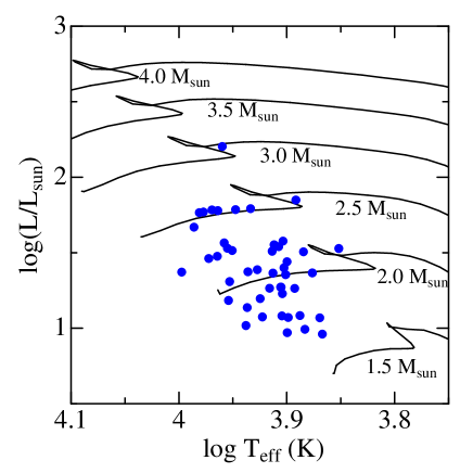
Fig. 1.—: Plots of 46 program stars on the theoretical HR diagram ($\log(L/L_{\odot})$ vs. $\log T_{\rm eff}$ ), where the bolometric luminosity ($L$) was evaluated from the apparent visual magnitude with the help of Hipparcos parallax (ESA 1997) and Flower’s (1996) bolometric correction. Theoretical evolutionary tracks corresponding to the solar metallicity computed by Girardi et al. (2000) for six different initial masses are also depicted for comparison.

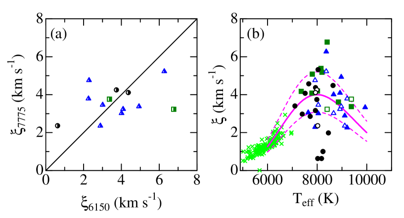
Fig. 2.—: (a) Comparison of the microturbulence derived from the 7775 region ($\xi_{7775}$) with that from the 6150 region ($\xi_{6150}$). (b) Microturbulences plotted against the effective temperature, where $\xi_{6150}$ and $\xi_{7775}$ are denoted by filled and open symbols, respectively. The results for F–G–K dwarfs taken from Takeda et al. (2005b) are also shown by crosses for comparison. In both panels, three groups of projected rotational velocity are discerned by the symbol shape: Triangles $\cdots$ slow rotators (0 km s${}^{-1}<v_{\rm e}\sin i<$ 50 km s^-1), squares $\cdots$ moderate rotators (50 km s${}^{-1}<v_{\rm e}\sin i<$ 100 km s^-1), and circles $\cdots$ rapid rotators (100 km s${}^{-1}<v_{\rm e}\sin i$). The adopted $\xi$ vs. $T_{\rm eff}$ relation [cf. Equation (1)] is depicted by solid line, while its reasonable upper and lower limits (perturbations by $\pm 30\%$ as possible range of errors) are shown by two dashed lines.

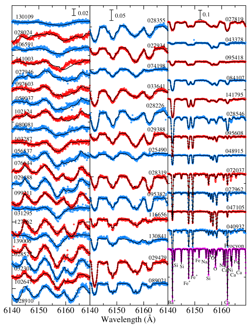
Fig. 3.—: Synthetic spectrum fitting at the 6150 region (6140–6170 $\rm\AA$) for determining the projected rotational velocity ($v_{\rm e}\sin i$) and the abundances of O, Si, Ca, Fe, and Ba. The best-fit theoretical spectra are shown by solid lines, while the observed data are plotted by symbols. Left panel $\cdots$ rapid rotators (100 km s${}^{-1}<v_{\rm e}\sin i$), middle panel $\cdots$ moderate rotators (50 km s${}^{-1}<v_{\rm e}\sin i<$ 100 km s^-1), and right panel $\cdots$ slow rotators (0 km s${}^{-1}<v_{\rm e}\sin i<$ 50 km s^-1). In each panel, the spectra are arranged in the descending order of $v_{\rm e}\sin i$, and an appropriate offset is applied to each spectrum (indicated by the HD number) relative to the adjacent one. The case of Procyon (standard star) is displayed at the bottom of the right panel.

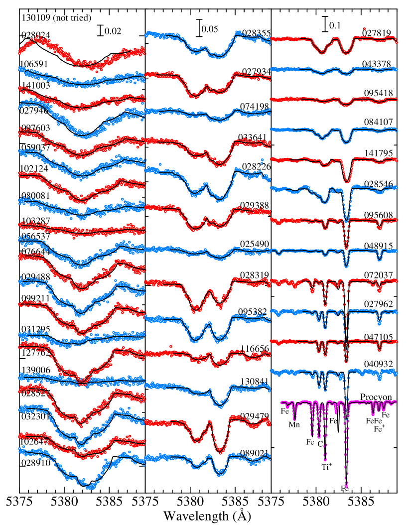
Fig. 4.—: Synthetic spectrum fitting at the 5380 region (5375–5390 $\rm\AA$) for determining $v_{\rm e}\sin i$ and the abundances of C, Ti, and Fe. Otherwise, the same as in Fig. 3.

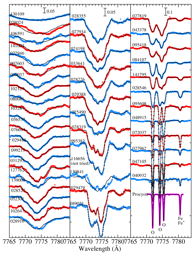
Fig. 5.—: Synthetic spectrum fitting at the 7775 region (7765–7785 $\rm\AA$) for determining $v_{\rm e}\sin i$ and the abundances of O (with the non-LTE effect taken into account) and Fe. Otherwise, the same as in Fig. 3.

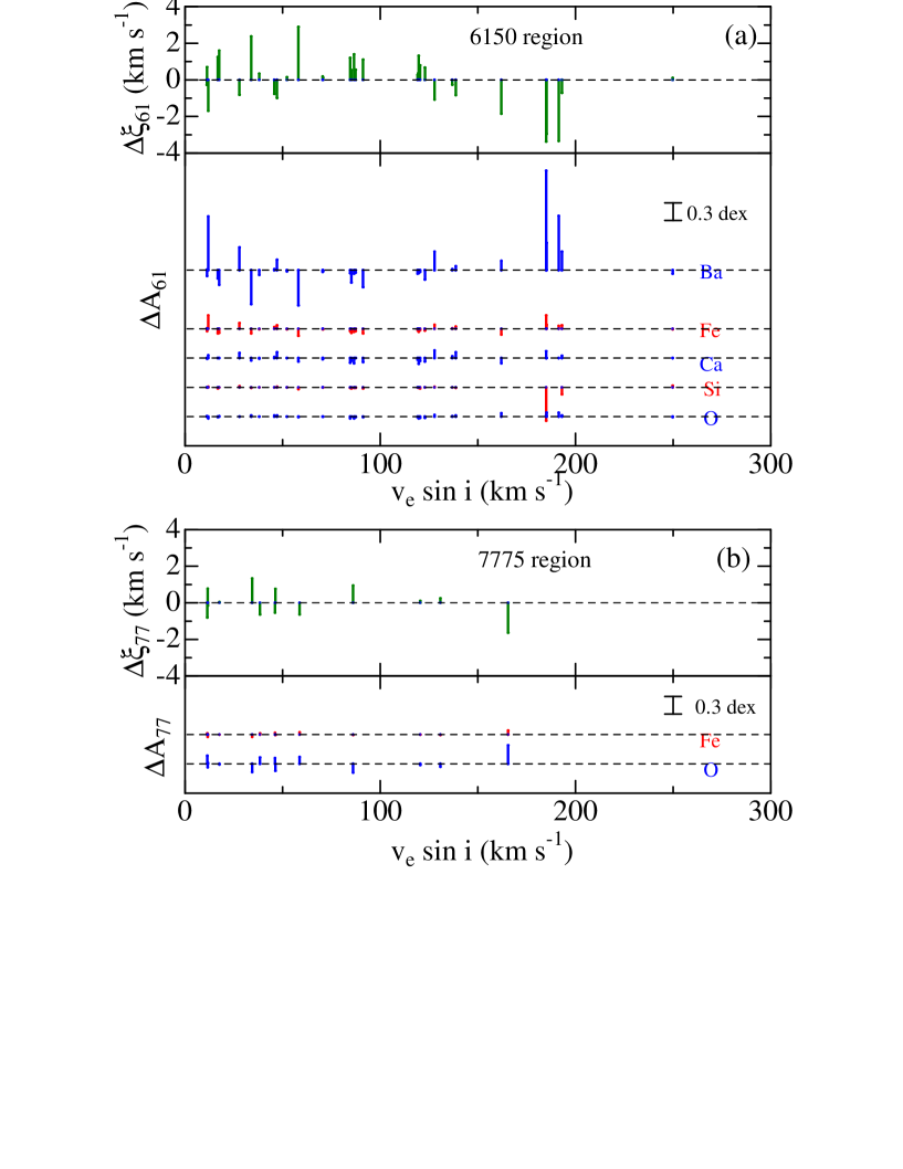
Fig. 6.—: Abundance changes between the two cases of $\xi^{\rm fit}$ and $\xi^{\rm std}$ [$\Delta A\equiv A(\xi^{\rm fit})-A(\xi^{\rm std})$] plotted as functions of $v_{\rm e}\sin i$. (a) 6150 region (33 stars) and (b) 7775 region (13 stars). In each figure, the upper and lower panels show $\Delta\xi\equiv(\xi^{\rm fit}-\xi^{\rm std})$ and $\Delta A$ (for each element), respectively.

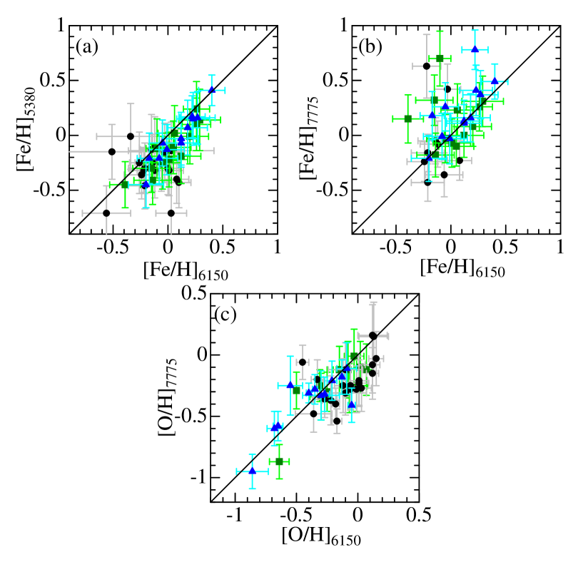
Fig. 7.—: Comparisons of the abundances derived from different regions (cf. Table 1). (a) [Fe/H]₅₃₈₀ vs. [Fe/H]₆₁₅₀, (b) [Fe/H]₇₇₇₅ vs. [Fe/H]₆₁₅₀, and (c) [O/H]₇₇₇₅ vs. [O/H]₆₁₅₀. The error bars attached in [X/H] represent the values of $\Delta A^{\rm X}$ (see Sect. IV-c). Three groups of different $v_{\rm e}\sin i$ ranges are discriminated by the symbol shape in the same manner as in Fig. 2.

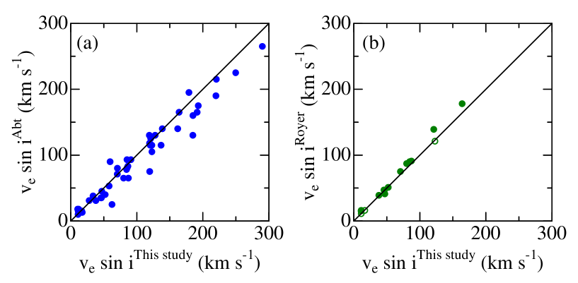
Fig. 8.—: Comparison of the $v_{\rm e}\sin i$ results derived in this study (determined from the fitting in the 6150 region; cf. Table 1). with the literature values: (a) Abt & Morrell (1995), (b) Royer et al. (2002a; open symbols; southern hemisphere) and Royer et al. (2002b; filled symbols; northern hemisphere).

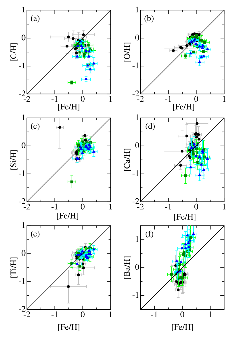
Fig. 9.—: [X/H] values plotted against [Fe/H] (6150 region). (a) [C/H], (b) [O/H] (6150 region), (c) [Si/H], (d) [Ca/H], (e) [Ti/H], and (f) [Ba/H]. The error bars attached in [X/H] represent the values of $\Delta A^{\rm X}$ (see Sect. IV-c). See the caption of Fig. 2 for the meanings of the symbols.

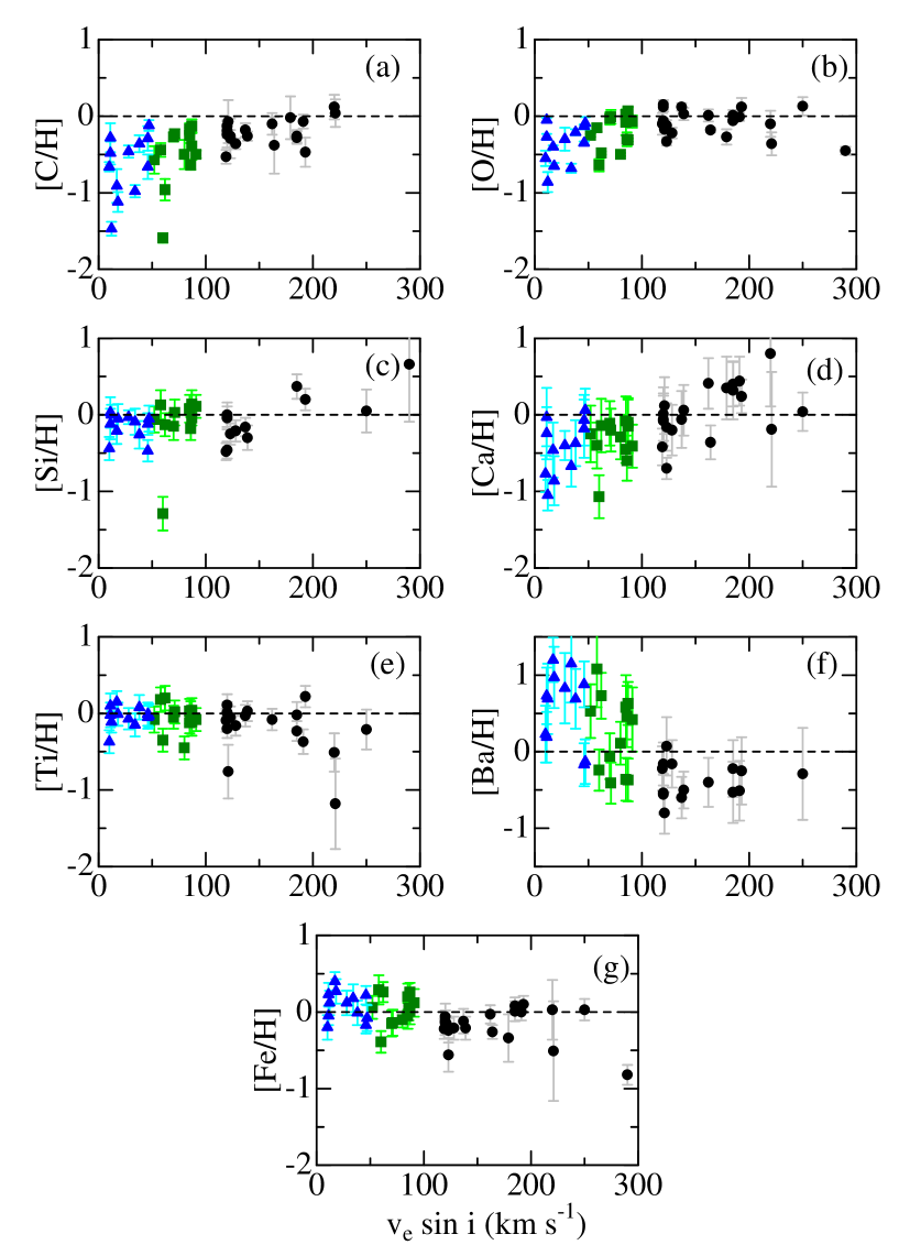
Fig. 10.—: [X/H] values plotted against $v_{\rm e}\sin i$ (6150 region). (a) [C/H], (b) [O/H] (6150 region), (c) [Si/H], (d) [Ca/H], (e) [Ti/H], (f) [Ba/H], and (g) [Fe/H] (6150 region). The error bars attached in [X/H] represent the values of $\Delta A^{\rm X}$ (see Sect. IV-c). See the caption of Fig. 2 for the meanings of the symbols.

References

- Abt, H. A., & Morrell, N. I. 1995, ApJS, 99, 135
- Allende Prieto, C., Barklem, P. S., Lambert, D. L., & Cunha, K. 2004, A&A, 420, 183
- Andrievsky, S. M., et al. 2002, A&A, 396, 641
- Asplund, M., Grevesse, N., Sauval, A. J., Allende Prieto, C., & Kiselman, D. 2004, A&A, 417, 751
- Cayrel de Strobel, G., Soubiran, C., & Ralite, N. 2001, A&A, 373, 159
- Coupry, M. F., & Burkhart, C. 1992, A&AS, 95, 41
- Dunkin, S. K., Barlow, M. J., & Ryan, S. G. 1997, MNRAS, 286, 604
- Edvardsson, B., Andersen, J., Gustafsson, B., Lambert, D. L., Nissen, P. E., & Tomkin, J. 1993, A&A, 275, 101
- ESA 1997, The Hipparcos and Tycho Catalogues, ESA SP-1200, available from NASA-ADC or CDS in a machine-readable form (file name: hip_main.dat)
- Flower, P. J. 1996, ApJ, 469, 355
- Fossati, L., Bagnulo, S., Landstreet, J., Wade, G., Kochukhov, O., Monier, R., Weiss, W., & Gebran, M. 2008, A&A, 483, 891
- Gebran, M., Monier, R., & Richard, O. 2008, A&A, 479, 189
- Gebran, M., & Monier, R. 2007, in Convection in Astrophysics, ed. F. Kupka, I. W. Roxburgh, & K. L. Chan, Proc. IAU Symp. 239 (Cambridge: Cambridge University Press), 160
- Gebran, M., & Monier, R. 2008, A&A, 483, 567
- Gies, D. R., & Lambert, D. L. 1992, ApJ, 387, 673
- Girardi, L., Bressan, A., Bertelli, G., & Chiosi, C. 2000, A&AS, 141, 371
- Hauck, B., & Mermilliod, M. 1980, A&AS, 40, 1
- Kang, D.-I., Park, H.-S., Han, I.-W., Valyavin, G., Lee, B.-C., & Kim, K.-M. 2006, PKAS, 21, 101
- Kato, K., & Sadakane, K. 1982, A&A, 113, 135
- Kilian, J. 1992, A&A, 262, 171
- Kilian, J. 1994, A&A, 282, 867
- Kurucz, R. L. 1993, Kurucz CD-ROM, No. 13 (Harvard-Smithsonian Center for Astrophysics)
- Kurucz, R. L., & Bell, B. 1995, Kurucz CD-ROM, No. 23 (Harvard-Smithsonian Center for Astrophysics)
- Kurucz, R. L., & Peytremann, E. 1975, Smithsonian Astrophys. Obs. Spec. Rept., No. 362
- Lemke, M. 1990, in The Atmospheres of Early-Type Stars, ed. U. Heber & C. S. Jeffery (Berlin: Springer), p.54
- Lemke, M. 1993, in Peculiar versus Normal Phenomena in A-type and Related Stars, eds. M.M. Dworetsky, F. Castelli, & R. Faraggiana (San Francisco: Astronomical Society of the Pacific), p.407
- Luck, R. E., & Lambert, D. L. 1985, ApJ, 298, 782
- Moon, T. T. 1985, Commun. Univ. London Obs., No. 78
- Napiwotzki, R., Schönberner, D., & Wenske, V. 1993, A&A, 268, 653
- Niemczura, E. 2003, A&A, 404, 689
- Nissen, P. E. 1993, in Inside the stars, ASP Conf. Ser. 40, eds. W. W. Weiss & A. Baglin, (San Francisco: Astronomical Society of the Pacific), p. 108
- Royer, F., Gerbaldi, M., Faraggiana, R., & Gómez, A. E. 2002a, A&A, 381, 105
- Royer, F., Grenier, S., Baylac, M.-O., Gómez, A. E., & Zorec, J. 2002b, A&A, 393, 897
- Sadakane, K. 1990, in Accuracy of element abundances from stellar atmospheres, Lecture Note in Physics, No. 356, ed. R. Wehrse (Berlin and New York: Springer), 57
- Sadakane, K., & Okyudo, M. 1989, PASJ, 41, 1055
- Savanov, I. S. 1995a, Astron. Rep., 39, 653
- Savanov, I. S. 1995b, Astron. Lett., 21, 684
- Steffen, M. 1985, A&AS, 59, 403
- Takeda, Y. 1995, PASJ, 47, 287
- Takeda, Y. 2003, A&A, 402, 343
- Takeda, Y., et al. 2005a, PASJ, 57, 13
- Takeda, Y., & Honda, S. 2005, PASJ, 57, 65
- Takeda, Y., Ohkubo, M., Sato, B., Kambe, E., & Sadakane, K. 2005b, PASJ, 57, 27 [Erratum: PASJ, 57, 415]
- Takeda, Y., & Sadakane, K. 1997, PASJ, 49, 367
- Takeda, Y., Sato, B., & Murata, D. 2008, PASJ, 60, 781
- Takeda, Y., & Takada-Hidai, M. 1998, PASJ, 50, 629
- Takeda, Y., Takada-Hidai, M., Jugaku, J., Sakaue, A., & Sadakane, K. 1999, PASJ, 51, 961
- Varenne, O., & Monier, R. 1999, A&A, 351, 247
- Young, P. R. 2005, A&A, 444, L45