Orbital Selective Superconductivity in Two-Orbital Asymmetric t-J Models

Abstract

We present the zero-temperature superconducting (SC) ground states of the two-orbital asymmetric $t-J$ model on a square lattice by means of the auxiliary-boson approach. Besides the two-gap SC phase, we find an orbital selective SC (OSSC) phase, which is simultaneously SC in one orbit and normal in another orbit. The novel OSSC phase is stable only for sufficient asymmetric degree in orbital space and doping concentration. The pairing symmetry of the SC phase is $s$-wave-like in most doping regime, against the $d$-wave symmetry of the single-orbital $t-J$ model in a square lattice. The implication of the present scenario on the iron-based and other multi-orbital superconductors is also discussed.

I Introduction

Searching high-T_c superconducting states in correlated electron systems has been one of the central topics in condensed matter physics for several decades Lee0 . With the development of synthesis technique, more and more new superconducting (SC) compounds have been discovered, such as UGe₂ Saxena ; Huxley and URhGe Aoki with the coexistence of ferromagnetism and SC, and LaO_0.9F_0.1FeAs with the anomalous Hall coefficient and magnetoresistance in the SC Hosono ; Yang , etc. Among the fantastic properties of these compounds, the multi-gap SC nature is one of the most interested. The multi-gap SC characters have been found in a number of compounds, for example, in nodal structure Sr₂RuO₄Maeno ; Mackenzie , in $s$-wave SC NbSe₂Yokoya ; Boaknin and MgB₂ Canfield ; Blumberg ; Iavarone , in heavy-fermion SC Ce_1-xLa_xCoIn₅ Tanatar ; Flouquet , and in d-wave SC PbBi₂Sr₂CuO_6+xBoyer and Bi2212 Lee . Recently, a generic two-gap hypothesis is also proposed for the cuprate SC Sawatzky . Further, in the iron-based SC discovered recently Hosono , some experiments also showed that LaO_1-xF_xFeAs is two-gap SC Mandrus ; Zhenggq . On the other hand, in the heavy-fermion SC Ce_1-xLa_xCoIn₅ Tanatar ; Flouquet , it is found recently that there coexist uncondensed carriers and the SC carriers, and a fraction of electrons on the Fermi surfaces does not participate in SC, displaying unusual SC characteristics in Ce_1-xLa_xCoIn₅. Since these compounds share the same properties in the electronic structures, i.e., the multi-orbital or multi-band character Agterberg ; Liu2 ; Barzykin , it naturally arises the question that whether the condensed and the uncondensed phases generally coexist in the multi-orbital SC compounds ?

In the past decade, it has been found that numerous correlated electron compounds are multi-orbital, and many unique features are contributed from the orbital degree of freedom, such as colossal magnetoresistance and complex orbital ordered phases in doped manganitesImada , the exotic magnetism in the $f$-electron systems Santini , and the debated orbital selective Mott transition (OSMT) in Sr_2-xCa_xRuO₄ Anisimov ; Nakatsuji ; Lee2 ; Wang ; Dai , $etc.$ The orbital degree of freedom on the SC plays an important role in the SC pairing symmetry of the multi-orbital systems Takimoto ; Takimoto2 ; Mochizuki ; Kubo . On the other hand, Liu $et$ $al.$Liu proposed that there may exist an interior gap superfluidity in a two-orbital system, in which the pairing interaction carves out a gap within the interior of a large Fermi ball, while the exterior surface remains gapless; and it is a simultaneously SC and normal state at zero temperature. Nevertheless, the role of orbital degree of freedom on the pairing symmetry and SC condensation is far from well understood. So, much effort is still needed to uncover the SC nature in strongly correlated multi-orbital compounds.

With this motivation, and stimulated by searching for a new state of matter, we study the SC properties of the strongly correlated multi-orbital systems in this paper. We extend the single-orbital $t-J$ model to the two-orbital $t-J$ model, and utilize the auxiliary-boson method Coleman to obtain the phase diagram of the system on a square lattice. We find that for given strong interactions between electrons, the electrons may bind as many paired quasiparticles as possible in one orbit due to the symmetry breaking in the orbital space. These quasiparticles condense into a coherent state at low temperature, and the residual unpaired electrons in the other orbit constitute a separated normal fluid, forming the orbital selective SC (OSSC) phase. The OSSC phase is the stablest, against to the normal phase and the full-gapped SC ones, in proper parametric and doping regime. We also obtain the critical points of the formation of OSSC phase for various parameters of the two-orbital $t-J$ model, which may shed light on finding this phase in the strongly correlated compounds. The possible application of the present theory on the Fe-based SC LaO_1-xF_xFeAs is also discussed.

The rest of this paper is organized as follows. In Sec.II, we describe the two-orbital $t-J$ model and the framework of the auxiliary-boson mean field approach. And then we present the detailed formulation of the two-orbital SC. In Sec.III, we present the phase diagram of the SC in the two-orbital system. The conditions for the formation of the OSSC phase and its possible application on Ce_1-xLa_xCoIn₅ and Fe-based SC are discussed. The last part is devoted to the summary.

II HAMILTONIAN AND METHOD

The Hubbard model effectively describes the electronic correlations in the strongly interacting systems. In the single-orbital situation and in the strong correlation limit, the Hubbard model is reduced to an effective model describing the low-energy processes, i.e. the single-orbital $t-J$ modelAnderson ; Baskaran . In the strongly correlated multi-orbital systemCastellani , we naturally extend the single-orbital $t-J$ model to the multi-orbital t-J model described by the Hamiltonian

$$H = P[H_{t}+H_{J}]P.$$

with a kinetic energy part $H_{t}$

$$H_{t} = \sum_{<ij>mm^{\prime}\sigma}t_{ij}^{mm^{\prime}}(c^{\dagger}_{im\sigma}c_{jm\sigma}+h.c)+\sum_{i\sigma}E_{m}n_{im\sigma}$$

and a general superexchange coupling $H_{J}$ Castellani .

$$H_{J} =-\sum_{<ij>\sigma}\sum_{nn^{\prime}m}c^{\dagger}_{in\sigma}c_{in^{\prime}\sigma}[J^{nmn^{\prime}m}_{1}(n_{jm\bar{\sigma}}+c^{\dagger}_{jm\bar{\sigma}}c_{jm\sigma})$$

$$+(J^{nmn^{\prime}m}_{2}n_{j\bar{m}\bar{\sigma}}+J^{nmn^{\prime}\bar{m}}_{2}c^{\dagger}_{j\bar{m}\bar{\sigma}}c_{jm\sigma})$$

$$+(J^{nmn^{\prime}m}_{3}n_{j\bar{m}\sigma}+J^{nmn^{\prime}\bar{m}}_{3}c^{\dagger}_{j\bar{m}\sigma}c_{jm\sigma})$$

$$-(J^{nmn^{\prime}m}_{4}c^{\dagger}_{j\bar{m}\bar{\sigma}}c_{j\bar{m}\sigma}-J^{nmn^{\prime}\bar{m}}_{4}c^{\dagger}_{j\bar{m}\bar{\sigma}}c_{jm\bar{\sigma}})$$

$$+(J^{nmn^{\prime}\bar{m}}_{5}c^{\dagger}_{jm\bar{\sigma}}c_{j\bar{m}\bar{\sigma}}-J^{nmn^{\prime}\bar{m}}_{5}c^{\dagger}_{jm\bar{\sigma}}c_{j\bar{m}\sigma})],$$

where $c^{\dagger}_{im\sigma}(c_{im\sigma})$ is the creation (annihilation) operator of the electron at site $i$ with orbit-m and spin $\sigma(=\uparrow,\downarrow)$; and $\bar{m}$ ($\bar{\sigma}$) denotes the orbit (spin) other than m ($\sigma$). $n_{im\sigma}(=c^{\dagger}_{im\sigma}c_{im\sigma})$ is the electron number operator. E_m denotes the crystalline field level of the orbit-$m$. The operator $P$ projects out the states of multiple occupancy at each site. Therefore, every site is either spin 1/2 or a vacancy. $t_{ij}^{nm}$ denotes the hopping integral from the $m$ orbit at site j to the $n$ orbit at site i, and only the nearest-neighbor hopping is taken into account. In this paper, we define $t_{ij}^{11}=t=1$ as the energy unit. The parameter J${}^{nmn^{\prime}m^{\prime}}$ is associated with the hopping integrals t^nm, the on-site and inter-orbital Coulomb interactions $U$ and $U^{\prime}$, and the Hund’s coupling via, $J^{nmn^{\prime}m^{\prime}}_{1}={t_{ij}^{nm}t_{ij}^{n^{\prime}m^{\prime}}U}/{(U^{2}-J^{2})}$, $J^{nmn^{\prime}m^{\prime}}_{2}={t_{ij}^{nm}t_{ij}^{n^{\prime}m^{\prime}}U^{\prime}}/{(U{{}^{\prime}}^{2}-J^{2})}$, $J^{nmn^{\prime}m^{\prime}}_{3}={t_{ij}^{nm}t_{ij}^{n^{\prime}m^{\prime}}}/{(U{{}^{\prime}}-J)}$, $J^{nmn^{\prime}m^{\prime}}_{4}={t_{ij}^{nm}t_{ij}^{n^{\prime}m^{\prime}}J}/{(U{{}^{\prime}}^{2}-J^{2})}$, $J^{nmn^{\prime}m^{\prime}}_{5}={t_{ij}^{nm}t_{ij}^{n^{\prime}m^{\prime}}J}/{(U^{2}-J^{2})}$. In what follows, considering the spin rotational symmetry, we adopt the relationship $U=U^{\prime}+2J$Castellani , and the system is on a square lattice.

Eq.(1) is a general multi-orbital $t-J$ Hamiltonian with the electron/hole filling not far from 1/4. In the absence of the Hund’s coupling and let the hopping integrals be isotropic for all of the orbits, Eq.(1) reduces to a supersymmetric SU(4) $t-J$ model Fujii ; Schlottmann . If the crystalline field splitting, $E_{\Delta}$=$E_{2}-E_{1}$, is sufficiently large, only the orbit/band m=1 is occupied, and Eq.(1) reduces to the traditional single-orbital $t-J$ model. For clarify, we concentrate on the two-orbital situation (m=1,2) without only the off-diagonal hoppings (t¹²=0) and the Hund’s coupling ($J=0$). Thus the effective Hamiltonian $H_{eff}$ in Eq.(1) becomes,

$$H_{t} = \sum_{<ij>m\sigma}t_{ij}^{mm}(c^{\dagger}_{im\sigma}c_{jm\sigma}+h.c)+E_{\Delta}\sum_{i\sigma}(n_{i1\sigma}-n_{i2\sigma})$$

$$H_{J} = -\sum_{<ij>\sigma}[J_{1}n_{i1\sigma}n_{j1\bar{\sigma}}+J_{2}n_{i2\sigma}n_{j2\bar{\sigma}}+(J_{1}+J_{2})$$ (4)

$$(n_{i1\sigma}n_{j2\bar{\sigma}}+n_{i1\sigma}n_{j2\sigma})-J_{1}c^{\dagger}_{i1\sigma}c_{i1\bar{\sigma}}c^{\dagger}_{j1\bar{\sigma}}c_{j1\sigma}$$

$$-J_{2}c^{\dagger}_{i2\sigma}c_{i2\bar{\sigma}}c^{\dagger}_{j2\bar{\sigma}}c_{j2\sigma}-2J_{3}(c^{\dagger}_{i1\sigma}c_{i2\sigma}c^{\dagger}_{j2\sigma}c_{j1\sigma}$$

$$-c^{\dagger}_{i1\sigma}c_{i2\bar{\sigma}}c^{\dagger}_{j2\bar{\sigma}}c_{j1\sigma})],$$

with $J_{1}=(t^{11})^{2}/U$, $J_{2}=(t^{22})^{2}/U$ and $J_{3}=t^{11}t^{22}/U$. To enforce the single occupation constraint at each site, we employ the auxiliary-boson mean-field approximation Kotliar on Eq.(4).

Within the slave-boson representation, the Hamiltonian (4) is rewritten in terms of the projected fermion operators $Pc^{\dagger}_{im\sigma}P$ and $Pc_{im\sigma}P$, which rule out the double and multiple fermion occupancies at every site, as well as the slave boson operators. The constrained Hilbert space ($S$) of each site $i$ is

$$S_{i}=\{{\mid 1,\uparrow>},{\mid 1,\downarrow>},{\mid 2,\uparrow>},{\mid 2,\downarrow>},{\mid 0,0>}\},$$ (5)

including the states of spin-up, spin-down in the orbit-1, and those in the orbit-2, together with vacancy state, respectively. The present constrained spin-orbital formulation resembles to the 4-fold degenerate state of pseudo-angular momentum $j$=$3/2$ proposed by ColemanColeman , if we define $\mid f^{0}>$=$\mid 0,0>$, ${\mid f^{1}:3/2,-3/2>}$=${\mid 1,\uparrow>}$, ${\mid f^{1}:3/2,-1/2>}$=${\mid 1,\downarrow>}$, ${\mid f^{1}:3/2,1/2>}$=${\mid 2,\uparrow>}$, and ${\mid f^{1}:3/2,3/2>}$=${\mid 2,\downarrow>}$. One obtains $Pc^{\dagger}_{im\sigma}P=f^{\dagger}_{im\sigma}.$ The boson operator $b_{i}^{\dagger}$ creates an empty occupation state at the $i$th site, and the fermion operator $f_{im\sigma}^{\dagger}(f_{im\sigma})$ creates (annihilates) a slaved electron at site $i$ with orbit-m and spin $\sigma(=\uparrow,\downarrow)$.

In the present situation, we define the SC order parameters as

$$\Delta^{\sigma,m}_{x/y} = <f^{\dagger}_{im\sigma}f^{\dagger}_{jm\bar{\sigma}}-f^{\dagger}_{im\bar{\sigma}}f^{\dagger}_{jm\sigma}>,(j=i\pm\hat{x}/\hat{y})$$

$${P_{m\sigma}} = <f^{\dagger}_{im\sigma}f_{jm\sigma}>,~{}{\bar{n}_{im\sigma}}=<f^{\dagger}_{im\sigma}f_{im\sigma}>$$ (6)

Considering the asymmetry of the orbital space and the Fermi surface topology, the $p$-wave SC order parameters vanish. In the mean-field or saddle-point approximation, we have $<b^{\dagger}_{i}b_{j}>=\mid b\mid^{2}=\delta$, and the electron filling n=1-$\delta$. Thus, we obtain the slave-boson mean-field Hamiltonian

$$H =E_{0}+\sum_{{\bf k}\sigma}\epsilon_{{\bf k}1\sigma}f^{\dagger}_{{\bf k}1\sigma}f_{{\bf k}1\sigma}-\sum_{{\bf k}\sigma}(\Delta^{\sigma 1}_{\bf k}f^{\dagger}_{{\bf k}1\sigma}f^{\dagger}_{{\bf-k}1\bar{\sigma}}+h.c)$$ (7)

$$+\sum_{{\bf k}\sigma}\epsilon_{{\bf k}2\sigma}f^{\dagger}_{{\bf k}2\sigma}f_{{\bf k}2\sigma}-\sum_{{\bf k}\sigma}(\Delta^{\sigma 2}_{\bf k}f^{\dagger}_{{\bf k}2\sigma}f^{\dagger}_{{\bf-k}2\bar{\sigma}}+h.c)$$

with the constant energy

$$E_{0} = N\sum_{\sigma}[2J_{1}\bar{n}_{1\sigma}\bar{n}_{1\bar{\sigma}}+\genfrac{}{}{}{}{J_{1}}{2}(\mid\Delta^{\sigma 1}_{x}\mid^{2}+\mid\Delta^{\sigma 1}_{y}\mid^{2})$$ (8)

$$+2J_{1}P_{1\sigma}P_{1\bar{\sigma}}+2J_{2}\bar{n}_{2\sigma}\bar{n}_{2\bar{\sigma}}+\genfrac{}{}{}{}{J_{2}}{2}(\mid\Delta^{\sigma 2}_{x}\mid^{2}+\mid\Delta^{\sigma 2}_{y}\mid^{2})$$

$$+2J_{2}P_{2\sigma}P_{2\bar{\sigma}}+2(J_{1}+J_{2})(\bar{n}_{1\sigma}\bar{n}_{2\sigma}+\bar{n}_{1\sigma}\bar{n}_{2\bar{\sigma}})$$

$$+4J_{3}(P_{1\sigma}P_{2\sigma}+P_{1\sigma}P_{2\bar{\sigma}})]$$

and the notations

$$\epsilon_{{\bf k}m\sigma} = -2[t_{m}\delta+(J_{m}P_{m\bar{\sigma}}+J_{3}P_{\bar{m}\sigma}+J_{3}P_{\bar{m}\bar{\sigma}})]\gamma_{\bf k}-\mu$$

$$-2[2J_{m}\bar{n}_{m\bar{\sigma}}+(J_{1}+J_{2})(\bar{n}_{\bar{m}\sigma}+\bar{n}_{\bar{m}\bar{\sigma}})]+E_{\Delta},$$

$$\Delta^{\sigma m}_{\bf k} = J_{m}[\Delta^{\sigma m}_{x}cos(k_{x}a)+\Delta^{\sigma m}_{y}cos(k_{y}a)],$$

$$\gamma_{\bf k} = cos(k_{x}a)+cos(k_{y}a).$$ (9)

Diagonalizing Eq.(8) through the Valatin transformation Valatin ; Callaway .

$$f_{{\bf k}m\uparrow} = U_{{\bf k}m}{\alpha}_{{\bf k}m}+V_{{\bf k}m}\beta^{\dagger}_{{\bf k}m},$$

$$f_{{\bf-k}m\downarrow} = U_{{\bf k}m}{\beta}_{{\bf k}m}-V_{{\bf k}m}\alpha^{\dagger}_{{\bf k}m},$$ (10)

with $U_{{\bf k}m}^{2}+V_{{\bf k}m}^{2}=1$, here $U_{{\bf k}m}$ and $V_{{\bf k}m}$ (m=1,2) are real and positive. The slave-boson mean-field Hamiltonian becomes

$$H = \sum_{\bf k}[\xi_{{\bf k}1}(\alpha^{\dagger}_{{\bf k}1}\alpha_{{\bf k}1}+\beta^{\dagger}_{{\bf k}1}\beta_{{\bf k}1})+\xi_{{\bf k}2}(\alpha^{\dagger}_{{\bf k}2}\alpha_{{\bf k}2}+\beta^{\dagger}_{{\bf k}2}\beta_{{\bf k}2})]$$ (11)

$$+E_{0}+\sum_{\bf k}[(\epsilon_{{\bf k}1}-\xi_{{\bf k}1})+(\epsilon_{{\bf k}2}-\xi_{{\bf k}2})],$$

with the quasiparticle excitation spectrum,

$$\xi_{{\bf k}m\sigma}=\sqrt{\epsilon^{2}_{{\bf k}m\sigma}+4\mid\Delta^{\sigma m}_{\bf k}\mid^{2}},$$ (12)

and the chemical potential $\mu$ is determined by $1-\delta=1/N\sum_{im\sigma}<f^{\dagger}_{im\sigma}f_{im\sigma}>$. The order parameters P_mσ and $\Delta^{\sigma m}$ satisfy the self-consistent equations:

$$1 = \genfrac{}{}{}{}{t^{2}_{m}}{UN}\sum_{\bf k}\genfrac{}{}{}{}{(cos(k_{x}a)+cos(k_{y}a))^{2}}{\xi_{{\bf k}m}}$$

$$P_{m\sigma} = \genfrac{}{}{}{}{1}{4N}\sum_{\bf k}(1-\genfrac{}{}{}{}{\epsilon_{{\bf k}m\sigma}}{\xi_{{\bf k}m\sigma}})\gamma_{\bf k}$$ (13)

for the $s$-wave SC. In the d-wave SC situation, these equations are slightly different.

III RESULTS AND DISCUSSION

In this section, we present the essential properties of the SC and the phase diagram of the two-orbital $t-J$ model. Provided the two-orbital model is SU(2) symmetric in the spin space, we would have the relations for the single occupation amplitude $P_{m\uparrow}=P_{m\downarrow}=P_{m}$ and for the SC order parameters, $\Delta^{\uparrow,m}_{x}=-\Delta^{\downarrow,m}_{x}=\Delta_{m}$, and $\Delta^{\uparrow,m}_{y}=-\Delta^{\downarrow,m}_{y}$ (m=1,2). This will greatly simplify our discussion in what follows.

III.1 Stable SC Phase and its Pairing Symmetry

We firstly determine the stablest ground state of the two-orbital $t-J$ model with n=1-$\delta$ in a square lattice through comparing the groundstate energy of the possible GS candidates: the normal state with $\Delta_{m}$=0, the $d$-wave symmetric SC phase with $\Delta^{\uparrow,m}_{x}=-\Delta^{\uparrow,m}_{y}$, or the $s$-wave-like symmetric SC phase with $\Delta^{\uparrow,m}_{x}=\Delta^{\uparrow,m}_{y}$. Throughout this paper, we adopt the relationship $J_{1}=0.1$, $J_{2}=J_{1}R^{2}$ and $J_{1}=J_{3}R$, unless specific explanation. Here the ratio of the hopping integrals is defined as R = t₂₂/t₁₁. The larger R deviates from the unity, the larger asymmetry degree of the orbital space is. By minimizing the GS energy, we obtain phase diagrams of the systems for various parameters, such as the doping concentration $\delta$, the exchange parameters $J_{1}$ and the asymmetric ratio of the hopping integrals, R, and the orbital level splitting, $E_{\Delta}$. Our numerical results show that the energy of the $s$-wave-like SC state is lower than that of the $d$-wave state for all the situations we investigated. Out of this reason, we focus on the s-wave like symmetric order parameters of the multi-orbital $t-J$ model in the following. The ground state strongly depends on the doping, the orbital asymmetry ratio, the level splitting and the the superexchange coupling strength, as shown the following phase diagrams. These phase diagrams demonstrate that there exists a new SC phase that is simultaneously SC and normal at zero temperature, analogous to the interior gap superfluidity proposed by Liu $et$ $al.$ Liu .

III.2 Doping Dependence

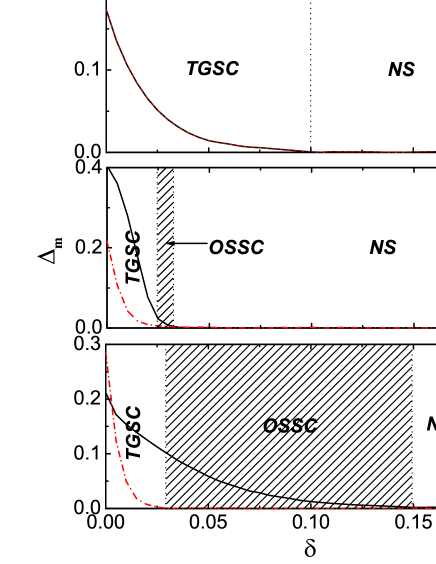
Figure 1: (Color online) The order parameters $\Delta_{m}$ (m=1,2) as functions of doping concentration $\delta$ for different situations, (a).$R=1$ and $\Delta=0$, (b).$R=0.3$ and $\Delta=0$, and (c).$R=1$ and $\Delta=0.1$, respectively.

We first present the evolution of the SC order parameters with the doping concentration. The order parameters $\Delta_{m}$ as the functions of doping $\delta$ in different parametric region are distinctly different, as shown in Fig. 1. When the system is SU(4) symmetric with $R=1$ and $E_{\Delta}=0$, it is clearly seen that the SC order parameters of the two orbits, $\Delta_{1}$ and $\Delta_{2}$, are equal. With the increase of doping $\delta$, the SC order parameters $\Delta_{1}$ and $\Delta_{2}$ simultaneously decrease and become zero at a critical value $\delta_{c}=0.09$, which is smaller than the critical value $\delta_{c}=0.32$ of the single-orbital $t-J$ model for SC phase. So, in the two-gap SC (TGSC) phase with SU(4) symmetry, the SC energy gaps of the two orbits are identical.

When the nearest-neighbor hoppings of the two orbits become asymmetric, such as, in the situation of $R=0.3$ and $E_{\Delta}=0$, we find that the order parameter of the orbit-1, $\Delta_{1}$, deviates from that of the orbit-2, $\Delta_{2}$. With the increase of $\delta$, the SC order parameter $\Delta_{2}$ in the narrow band firstly vanishes at a critical value, $\delta_{c}=0.025$. On the contrast, the SC order parameter $\Delta_{1}$ gradually decreases and becomes zero at $\delta_{c}=0.035$. Thus in the doping region $\delta<0.025$, the system is in the TGSC phase that both orbits/bands are SC. While in the region $0.025<\delta<0.035$, a novel phase appears, in which the wide orbit is SC, while the narrow orbit is in the normal phase. This new phase is called the orbital selective superconductive (OSSC) phase, as seen the shaded region in Fig. 1b. Since the degree of the broken symmetry is not large, such a phase, analogous to the interior gap superfluidityLiu , occurs only in a very narrow region in the phase diagram.

The symmetry breaking arising from the crystal field splitting E_Δ also leads to the stable OSSC phase. As shown in Fig.1c, the OSSC phase in the situation $R=1$ and $E_{\Delta}=0.1$ is more robust. In this situation, with the increase of $\delta$, both the SC order parameters $\Delta_{m\sigma}$ decrease asynchronously, as seen in Fig. 1c. $\Delta_{2}$ vanishes at $\delta_{c}=0.035$, and $\Delta_{1}$ vanishes at $\delta_{c}=0.14$. There also exist three different phases, the TGSC phase, the OSSC phase and the normal ones. Among these phases, the presence of crystalline field splitting favors the formation of the OSSC phase. We notice that in Fig.1, when the orbital rotational symmetry is broken, the SC order parameters at $\delta\rightarrow$ 0 are considerably larger than those with orbital rotational symmetry, demonstrating that the SC pairing strength may be enhanced by the orbital asymmetry, as we seen in next subsection.

III.3 Orbital Asymmetry Dependence

In fact, whether there exists the OSSC phase reflects the orbital symmetry of the systems. For $R=1$ and $E_{\Delta}=0$, the system has the SU(2) symmetry in the orbital space. In other words, there is no difference between the two orbits, their order parameters simultaneously decrease and vanish. Therefore, the TGSC and the normal phases are the stablest in this situation. Whilst, in the situations of $R=0.3$, $E_{\Delta}=0$ and $R=1$, $E_{\Delta}=0.1$, the rotation symmetry in the orbital space is broken because of the inequivalence of the two orbits for the case with $R=0.3$ and $E_{\Delta}=0$ or the case with $R=0$ and $E_{\Delta}=0.1$. The asymmetry of the two orbits leads to that the SC gaps of the two orbits are out of synchronization when approaching the critical points. For example, in the situation with $R=0.3$ and $E_{\Delta}=0$, due to the asymmetry of the two hopping integrals, the electrons in the narrow orbit feel weaker attractive interaction than those in the wide orbit, and forming a small SC gap. Thus, with the increasing of $\delta$, the electrons in the narrow orbit will first enter the normal state; at the same time, the electrons in the wide orbit may be still SC, as seen in Fig.1b and 1c.

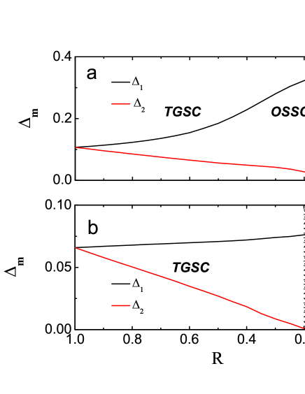
Figure 2: (Color online) The order parameters $\Delta_{m}$ (m=1,2) vs ratio of hopping integrals $R$ for different situations (a). $\delta=0.01$ and$\Delta=0$, and (b). $\delta=0.02$ and$\Delta=0$, respectively.

To get more insight to the behavior of the OSSC phase, we study how the phase diagram evolves with $R$, and the numerical result is shown in Fig. 2. In the system with $\delta=0.01$ and $E_{\Delta}=0$, it is clearly seen in Fig.2a that the difference between $\Delta_{1}$ and $\Delta_{2}$ increases with the deviation of $R$ from the unity. The SC order parameters exhibit different behavior: $\Delta_{2}$ monotonously increases and saturates at $R_{c}=0.08$; however, $\Delta_{1}$ monotonously decreases and vanishes at $R_{c}$, indicating the appearance of the OSSC phase. As the doping concentration increases to $\delta=0.02$ in Fig.2b, the two SC order parameters behave similar to the first situation. Finally, the TGSC-OSSC phase transition occurs at $R_{c}=0.22$. The critical value of the TGSC-OSSC phase transition becomes larger with the increase of $\delta$, in agreement with the results in Fig. 1. The asymmetric behavior of the SC order parameters arises from the symmetry breaking of the system in orbital space. Again, the asymmetry of the electron kinetic energy in two orbits favors the lift of the SC gap in the TGSC phase. When the hopping integral ratio R is greater than the unity, the behavior of $\Delta_{1}$ is inter-changed with that of $\Delta_{2}$.

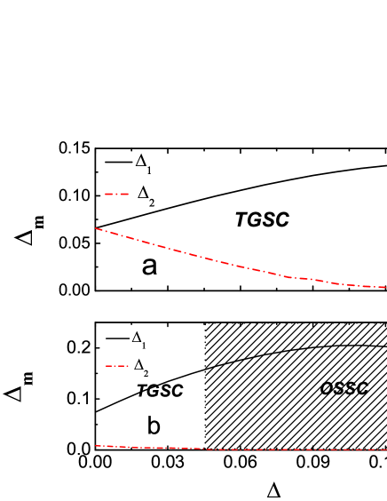
Figure 3: (Color online) Dependence of the SC order parameters $\Delta_{m}$ (m=1,2) on the level splitting $E_{\Delta}$ for (a). $R=1$ and $\delta=0.02$, and (b). $R=0.3$ and $\delta=0.02$, respectively.

III.4 Crystal Field Splitting Dependence of SC Phases

Not only the asymmetric hopping integrals, but also the crystalline field splitting $E_{\Delta}$ can break the orbital SU(2) symmetry of the system, leading to the formation of the OSSC phase, as seen in Fig.3. For the situation with $R=1$ and $\delta=0.02$ shown in Fig.3a, the positive crystalline field splitting $E_{\Delta}$ enhances the SC order parameter in orbit-1, $\Delta_{1}$, however, suppresses that in orbit-2, $\Delta_{2}$. The system is in the TGSC phase when $E_{\Delta}$ is lower than the critical value, $E_{\Delta}^{c}$=0.125. When the crystalline field splitting is greater than a critical value, $E_{\Delta}^{c}$=0.125, the order parameter $\Delta_{2}$ vanishes. The system enters the OSSC regime. For the situation with $R=0.3$, the phase diagram is shown in Fig.3b. Compared with the situation in Fig.3a, the difference between the SC order parameters $\Delta_{1}$ and $\Delta_{2}$ is so significant that $\Delta_{2}$ is negligible as $E_{\Delta}>$ 0.042, implying that the OSSC phase is more robust in the presence of the large level splitting and the orbital-rotational symmetry breaking.

For the situation with R=1, the negative crystalline field splitting E_Δ reverse the behavior of $\Delta_{1}$ and $\Delta_{2}$. We find that similar to the role of the rotation symmetry breaking in orbital space, the remove of the orbital level degeneracy by the crystalline field splitting also enhances the occurrence of the OSSC phase. Obviously, both of the cases break the symmetry of the orbital space. Therefore, the asymmetry of the two orbits favors the OSSC phase.

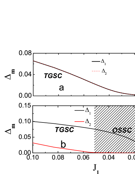
Figure 4: (Color online) The SC order parameters $\Delta_{m}$ (m=1,2) vs the superexchange coupling $J_{1}$ for different situations with $R=1$ and $\Delta=0$ (a), and $R=1$ and$\Delta=0.05$ (b), respectively, at $\delta=0.02$.

III.5 Superexchange Coupling Dependence

Similar to the single-orbital $t-J$ model Kotliar , when two superexchange pairing interactions $J_{1}$ and $J_{2}$ are too small, the normal state is stable against the SC phase, as shown in Fig.4a and Fig.4b. In the orbital SU(4) system with $R=1$ and $E_{\Delta}=0$, the SC order parameter of the orbit-1, $\Delta_{1}$, is equal to that of the orbit-2, $\Delta_{2}$, due to the symmetry in the orbital space. With the increase of the interaction strength $J_{1}$, the order parameters $\Delta_{m}$ (m=1,2) become finite at $J_{1c}=0.013$. The system lies in the TGSC regime. Under the situation of $R=1$ and $E_{\Delta}=0.05$, the order parameter $\Delta_{1}$ in the orbit-1 deviates from that in the orbit-2 due to the breaking of the orbital SU(2) symmetry. Compared with the case of the orbital SU(2) symmetry, a small crystal field splitting drives the narrow-band SC order parameter $\Delta_{2}$ to zero rapidly, and induces the occurrence of the OSSC-normal phase transition near the critical value $J_{1c}=0.05$.

From the discussion above, we have demonstrated that in proper parametric and doping regions, the OSSC phase is stablest, in comparison with the TGSC phase and the normal state in the multi-orbital $t-J$ model. The requirement condition for the occurrence of the OSSC phase is that the orbital SU(2) symmetry of the system is broken in the orbital space. Generally speaking, the larger the hopping integral ratio $R$ deviates from the unity, the larger the difference between two gaps is; so does the crystalline field splitting $E_{\Delta}$. Further, only in the proper doping and the interaction $J_{1}$ region, where the spin-fluctuation mediated pairing glue is strong enough, the system is stable in the OSSC state. One should recall that the present $s$-wave pairing symmetry is $cos(k_{x})+cos(k_{y})$-type, which exhibits nodes along the $k_{x}$=$k_{y}\pm\pi/2$, rather than the full-gapped BCS-type $s$-wave SC. Such a singlet pairing symmetry is also in agreement with Kubo’s result Kubo

The novelty of OSSC phase is the coexistence of the low-energy ”normal state” excitations and superconductivity. Such character could be manifested directly in the tunneling experiments, $i.e.$, the tunneling spectra may consist of those of the Cooper pairs and the normal electrons. To a certain extent, the OSSC phase is similar to the conventional SC with nodes, such as the $d$-wave SC cuprate, or the $p$-wave SC Sr₂RuO₄, $et$ $al.$ However, the OSSC phase differs from these states both quantitatively and qualitatively. Quantitatively, the DOS of OSSC phase is larger than those of the gapless modes; and qualitatively, the OSSC phase does not have the pairing symmetry of the $d$-wave or the $p$-wave SC. Although the OSSC state bears the resemblance to the interior gap superfluidity Liu , there is qualitative difference between these two states. Firstly, the microcosmic mechanisms of the superconductivity are different, since the present SC phases are mediated through the spin fluctuations, while the interior superfluid forms through the Bose-Einstein condensation. Secondly, the precondition of the interior gap superfluidity requires that the effective masses of the quasiparticle in the two branches is different; whilst, our theory predicts that the OSSC phase can exist even if the effective masses in both orbits are identical, providing that crystalline field splitting is large.

To date, no direct experimental observation about the novel OSSC phase is available. Nevertheless, we could find some hints in the anomalous properties of some unconventional SC. Recently, by measuring the thermal conductivity and the specific heat in the heavy-fermion SC Ce_1-xLa${}_{x}Co$In₅ Tanatar , Tanatar $et$ $al.$ proposed that in the doped compound, there coexist uncondensed electrons and nodal quasiparticles. And more recent thermal measurement Flouquet demonstrated that in undoped CeCoIn₅, there exists the multigap structure in the SC phase. From the present OSSC scenario, these two behaviors are consistent with each other, rather than contradict with each other. Since the number of orbits and the dispersion relation in CeCoIn₅ are different from the present simple model, more effort is needed to directly compare the present theory and experimental results in CeCoIn₅.

Furthermore, the Fe-based SC discovered recently may be another candidate of the OSSC phase. Some recent studies suggested that in undoped LaOFeAs, the electron correlation between Fe 3d electrons is strong and plays an important role in the ground state Kotliar2 ; Laad , and the first-principles electronic structure calculations suggest that two or more orbits are involved in the superconductivity, implying that the multi-orbital $t-J$ model is appropriate for describing the low-energy physics of the iron-based SC. With the increase of F-doping concentration, the system undergoes from the normal to the SC states. The two-gap character in sufficient F-doped LaOFeAs Mandrus ; Zhenggq suggests that in the some doping region, these may exist the unconventional SC phase. Surely, we expect that more elaborate experiments and the comparisons between the theory and the experiment can be performed to uncover the unconventional SC phase.

IV Conclusions

In summary, by using the extended auxiliary-boson approach, we have demonstrated that in the multi-orbital $t-J$ models, besides the two-gap superconducting phase, an orbital selective superconducting ground state may be stable, when the orbital SU(2) symmetry is broken in the correlated electronic systems. Such a new phase is s-wave like. The superconducting order parameters strongly depend on the asymmetry of the hopping $R$ and the crystal field splitting $E_{\Delta}$. The more the deviation from the orbital SU(2) symmetry is, the more robust the orbital selective superconducting phase is. Of course, the complicated dispersions relation of the multi-orbital systems in realistic compounds may lead to more interesting phenomena, and deserve further extensive investigation.

- (1) P. A. Lee, N. Nagaosa, and X. G. Wen, Rev. Mod. Phys. 78, 17 (2006).
- (2) S. S. Saxena, P. Agarwal, K. Ahilan, F. M. Grosche, R. K. W. Haselwimmer, M. J. Steiner, E. Pugh, I. R. Walker, S. R. Julian, P. Monthoux, G. G. Lonzarich, A. Huxley, I. Sheikin, D. Braithwaite, and J. Flouquet, Nature 406, 587 (2000).
- (3) A. Huxley, I. Sheikin, E. Ressouche, N. Kernavanois, D. Braithwaite, R. Calemczuk, and J. Flouquet, Phys. Rev. B 63, 144519 (2001).
- (4) D. Aoki, A. D. Huxley, E. Ressouche, D. Braithwaite, J. Flouquet, J. P. Brison, E. Lhotel, and C. Paulsen, Nature 413, 613 (2001).
- (5) H. Yang, X. Y Zhu, L. Fang, G. Mu, and H. H. Wen, cond-mat/08030623 (2008)
- (6) Y. Maeno, H. Hashimoto, K. Yoshida, S. Nishizaki, T. Fujita, J. G. Bednorz, and F. Lichtenberg, Nature 372, 532 (1994).
- (7) A. P. Mackenzie and Y. Maeno, Rev. Mod. Phys. 75, 657 (2003).
- (8) T. Yokoya et al, Science 294, 2518 (2001).
- (9) E. Boaknin et al, Phys. Rev. Lett. 90, 117003 (2003).
- (10) P. C. Canfield and G. W. Crabtree, Physics Today, 56, No.3, 34 (2003).
- (11) G. Blumberg, A. Mialitsin, B. S. Dennis, N. D. Zhigadlo, and J. Karpinski, Physica C 456 pp. 75-82 (2007).
- (12) M. Iavarone, G. Karapetrov, A. E. Koshelev, W. K. Kwok, G. W. Crabtree, and D. G. Hinks, cond-mat/0203329 (2002).
- (13) M. A. Tanatar, Johnpierre Paglione, S. Nakatsuji, D. G. Hawthorn, E. Boaknin, R. W. Hill, F. Ronning, M. Sutherland, Louis Taillefer, C. Petrovic, P. C. Canfield, Z. Fisk, Phys. Rev. Lett. 95, 067002 (2005)
- (14) G. Seyfarth, J. P. Brison, G. Knebel, D. Aoki, G. Lapertot and J. Flouquet, Phys. Rev. Lett. 101, 046401 (2008).
- (15) M. C. Boyer, W. D. Wise, Kamalesh Chatterjee, Ming Yi, Takeshi Kondo, T. Takeuchi, H. Ikuta, and E. W. Hudson, Nature Physics 3, 802 - 806 (2007)
- (16) W. S. Lee, I. M. Vishik, K. Tanaka, D. H. Lu, T. Sasagawa, N. Nagaosa, T. P. Devereaux, Z. Hussain, and Z.-X. Shen, Nature 450, 81 (2007).
- (17) S. Hufner, M. A. Hossain, A. Damascelli and G. A. Sawatzky, Rep. Prog. Phys. 71, 062501 (2008).
- (18) H. Takahashi, K. Igawa, K. Arii, Y. Kamihara, M. Hirano and H. Hosono, Nature 453, 376 (2008); X. H. Chen, T. Wu, G. Wu, R. H. Liu, H. Chen and D. F. Fang, Nature 453, 761 (2008).
- (19) F. Hunte, J. Jaroszynski, A. Gurevich, D.C. Larbalestier, R. Jin, A.S. Sefat, M.A. McGuire, B.C. Sales, D.K. Christen, D. Mandrus, Nature, 453, 903 (2008).
- (20) K. Matano, Z.A. Ren, X.L. Dong, L.L. Sun, Z.X. Zhao, Guo-qing Zheng, arXiv:0806.0249v1.
- (21) A. Y. Liu, I. I. Mazin, and J. Kortus, Phys. Rev. Lett. 87, 87005 (2001).
- (22) V. Barzykin and L. P. Gor’kov, cond-mat/0606191 (2006)
- (23) D. F. Agterberg, T. M. Rice, and M. Sigrist, Phys. Rev. Lett. 78, 3374 (1997).
- (24) V. Anisimov, I. Nekrasov, D. Kondakov, T. Rice and M. Sigrist, Eur. Phys. J. B 25, 191, (2002).
- (25) S. Nakatsuji and Y. Maeno, Phys. Rev. Lett. 84, 2666 (2000).
- (26) J. S. Lee, S. J. Moon, T.W. Noh, S. Nakatsuji, and Y. Maeno, Phys. Rev. Lett. 96, 057401 (2006).
- (27) S.-C. Wang et al., Phys. Rev. Lett. 93, 177007 (2004).
- (28) X. Dai et al., cond-mat/0611075v1 (2004).
- (29) M. Imada, A. Fujimori, and Y. Tokura, Rev. Mod. Phys. 70, 1039 (1998).
- (30) P. Santini, R. Lémanski, and P. Erdös, Adv. Phys. 48, 537 (1999).
- (31) W. Vincent Liu, and Frank Wilczek, Phys. Rev. Lett. 90, 047002 (2003).
- (32) T. Takimoto, Phys. Rev. B 62, R14641 (2000).
- (33) T. Takimoto, T. Hotta, and K. Ueda, Phys. Rev. B 69, 104504 (2004).
- (34) M. Mochizuki, Y. Yanase, and M. Ogata, Phys. Rev. Lett. 94, 147005 (2005).
- (35) K. Kubo, Phys. Rev. B 75, 224509 (2007).
- (36) P. W. Anderson, Nature 235, 1196 (1987).
- (37) G. Baskaran, Z. Zou, P. W. Anderson, Solid State Commun, 63, 973 (1987).
- (38) C. Castellani, C. R. Natoli and J. Ranninger, Phys. Rev. B. 18, 4945 (1978).
- (39) Feng Lu, Wei-Hua Wang and Liang-Jian Zou, Phys. Rev. B. 77, 125117 (2008).
- (40) Feng Lu, Dong-meng Chen and Liang-Jian Zou, cond-mat/0605379
- (41) T. Fujii, Y. Tsukamoto, and N. Kawakami, cond-mat/9811189
- (42) P. Schlottmann, Phys. Rev. Lett. 69, 2396 (1992).
- (43) G. Kotliar, and J, Liu, Phys. Rev. B. 38, 5142 (1988).
- (44) P. Coleman, Phys. Rev. B. 29, 3035 (1984), ibid 35, 5072 (1987)
- (45) D. G. Valatin, Nuovo Cimento 7, 843 (1958).
- (46) Joseph Callaway, Quantum theory of the solid state, Academic Press, (New York , 1976)
- (47) K. Haule, J. H. Shim and G. Kotliar, Phys. Rev. Lett. 100, 226402 (2008)
- (48) L. Craco, M. S. Laad, S. Leoni and H. Rosner, arXiv:0805.3636v1