Fluctuation-induced first-order transition in $p\,$-wave superconductors

Abstract

The problem of a fluctuation-induced first-order transition is considered for $p\,$-wave superconductors. Both an $\epsilon$-expansion about $d=4$ and a large-$n$ expansion conclude that the transition for the physical case $n=6$ in $d=3$ is of first order, as in the $s$-wave case.

I Introduction

BCS theory predicts that the phase transition from the normal state to the superconducting state in $s$-wave superconductors is continuous or second order. However, in 1974 Halperin, Lubensky, and Ma Halperin et al. (1974) argued, based on a $4-\epsilon$ expansion, that the coupling between the superconducting order parameter and the electromagnetic vector potential drives the transition first order. This conclusion is inevitable for extreme type-I superconductors where fluctuations of the order parameter are negligible and the vector potential can be integrated out exactly. The mechanism in this case is known as a fluctuation-induced first order transition, and it is analogous to the spontaneous mass generation known in particle physics as the Coleman-Weinberg mechanism.Coleman and Weinberg (1973) When order parameter fluctuations cannot be neglected, and especially for type-II superconductors, the problem cannot be solved exactly. The authors of Ref. Halperin et al., 1974 generalized the problem by considering an $n/2$-dimensional complex order parameter and conducting a renormalization-group (RG) analysis in $d=4-\epsilon$ dimensions. The physical case of interest is $n=2$ and $\epsilon=1$. To first order in $\epsilon$ they found that a RG fixed point corresponding to a continuous phase transition exists only for $n>365.9$, which suggests that for physical parameter values the transition is first order even in the type-II case. They corroborated this conclusion by performing a large-$n$ expansion for fixed $d=3$. To first order in $1/n$, the critical exponent $\nu$ is positive only for $n>9.72$, which again strongly suggests that the transition in the physical case $n=2$ is first order. For superconductors, due to the large correlation length and the correspondingly small size of the fluctuations, the size of the first order discontinuity is too small to be observable. For the analogous smectic-A to nematic transition in liquid crystals, on the other hand, it was predicted to be much larger, and, indeed, experimentally observable. In contrast to this theoretical prediction, experiments on liquid crystals showed, and continue to show to this day, a clear second order transition.Nounesis et al. (1993) This prompted a re-examination of the theory by Dasgupta and Halperin.Dasgupta and Halperin (1981) Using Monte Carlo data and duality arguments, these authors argued that a strongly type-II superconductor in $d=3$ should show a second order transition after all. A Monte-Carlo study of the intermediate region suggested that the transition is first order in the strongly type-I region and continuous in the strongly type-II region, with a tricritical point separating the two regimes.Bartholomew (1983) Why the continuous transition does not show as a critical fixed point in a $4-\epsilon$ expansion is not quite clear. One possible explanation is that the fixed point is not perturbatively accessible. Another is that the critical value of $n$ in the generalized model, which is close to 366 near $d=4$ where the $\epsilon$-expansion is controlled, decreases to a value less than 2 as the dimension is lowered to the physical value $d=3$. Herbut and TesanovicHerbut and Tesanovic (1996, 1997) have shown that the critical value of $n$, above which there is a second order transition, decreases rapidly with increasing $\epsilon$, and that a RG analysis in a fixed dimension $d=3$ to one-loop order does yield a critical fixed point for systems that are sufficiently strongly type II.

Recently there has been substantial interest in unconventional superconductivity. In particular, Sr₂RuO₄ has emerged as a convincing case of $p\,$-wave superconductivity,Nelson et al. (2004); Rice (2004) and UGe₂ is another candidate.Machida and Ohmi (2001) This raises the question whether for such systems the fluctuation-induced first order mechanism is also applicable, or whether the additional order parameter degrees of freedom allow for a critical RG fixed point, signalizing a second order transition, even though no such fixed point is found in the $s$-wave case. Here we investigate this problem. By conducting an analysis for $p\,$-wave superconductors analogous to the one of Ref. Halperin et al., 1974 we find that there is no critical fixed point, as in the $s$-wave case. This analysis thus also suggests a first order transition, as in the $s$-wave case, although the restrictions are somewhat less stringent. Presumably, the same reservations regarding non-perturbative fixed points that are suspected to be relevant for the $s$-wave case apply here as well.

This paper is organized as follows. In Sec. II we define our model and derive the mean-field phase diagram. In Sec. III we determine the nature of the phase transition. We do so first in a renormalized mean-field approximation that neglects fluctuations of the superconducting order parameter. We then take such fluctuations into account, first by means of a RG analysis in $d=4-\epsilon$ dimensions, and then by means of a $1/n$-expansion. In Sec. IV we summarize our results.

II Model

Let us consider a Landau-Ginzburg-Wilson (LGW) functional appropriate for describing spin-triplet superconducting order. The superconducting order parameter is conveniently written as a matrix in spin space, Vollhardt and Wölfle (1990) $\Delta_{\alpha\beta}({\bm{k}})=\sum_{\mu=1}^{3}d_{\mu}({\bm{k}})\left(\sigma_{\mu}i\sigma_{2}\right)_{\alpha\beta}$. Here $\sigma_{1,2,3}$ are the Pauli matrices, ${\bm{k}}$ is a wave vector, and the $d_{\mu}$ are the components of a complex $3$-vector ${\bm{d}}({\bm{k}})$. $p\,$-wave symmetry implies $d_{\mu}({\bm{k}})=\sum_{j=1}^{3}d_{\mu j}{\hat{k}}_{j}$, with $\hat{\bm{k}}$ a unit wave vector. The tensor field $d_{\mu j}({\bm{x}})$ is the general order parameter for a spin-triplet $p\,$-wave superconductor and it allows for a very rich phenomenology. For definiteness we will constrain our discussion to a simplified order parameter describing the so-called $\beta$-state,Vollhardt and Wölfle (1990) which has been proposed to be an appropriate description of UGe₂.Machida and Ohmi (2001) It is given by a tensor product $d={\bm{\psi}}\otimes{\bm{\phi}}$ of a complex vector ${\bm{\psi}}$ in spin space and a real unit vector ${\bm{\phi}}$ in orbital space. The ground state is given by ${\bm{\psi}}=\Delta_{0}(1,i,0)$, ${\bm{\phi}}=(0,0,1)$. In a weak-coupling approximation that neglects terms of higher than bilinear order in $\psi^{2}$, $\phi^{2}$, and $\nabla^{2}$ the action depends only on ${\bm{\psi}}$,

$$S = \int d{\bm{x}}\ \Bigl{[}t|{\bm{\psi}}|^{2}+c|{\bm{D}}{\bm{\psi}}|^{2}+u|{\bm{\psi}}|^{4}+v|{\bm{\psi}}\times{\bm{\psi}}^{*}|^{2}$$ (1)

$$\hskip 50.0pt+\frac{1}{8\pi\mu}({\bm{\nabla}}\times{\bm{A}})^{2}\Bigr{]}.$$

Here ${\bm{A}}$ is the vector potential, ${\bm{D}}={\bm{\nabla}}-iq{\bm{A}}$ is the gauge invariant gradient with $q=2e$ the Cooper pair charge (we use units such that Planck’s constant and the speed of light are unity), and $|{\bm{D}}{\bm{\psi}}|^{2}=(D_{i}\psi_{\alpha})(D_{i}^{*}\psi_{\alpha}^{*})$ with summations over $i$ and $\alpha$ implied. $\mu$ is the normal-state magnetic permeability, and $t$, $c$, $u$, and $v$ are the parameters of the LGW functional. The fields ${\bm{\psi}}$ and ${\bm{A}}$ are understood to be functions of the position ${\bm{x}}$.

For later reference we now generalize the vector ${\bm{\psi}}$ from a complex $3$-vector to a complex $m$-vector with components $\psi_{\alpha}$, so that the total number of order-parameter degrees of freedom is $n=2m$. In order to generalize the term with coupling constant $v$ we use of the following identity for $3$-vectors,

$$|{\bm{\psi}}\times{\bm{\psi}}^{*}|^{2}=\psi_{\alpha}\psi^{*}_{\alpha}\psi_{\beta}\psi^{*}_{\beta}-\psi_{\alpha}\psi_{\alpha}\psi^{*}_{\beta}\psi^{*}_{\beta}$$ (2)

and notice that the right-hand side is well defined for a complex $m$-vector. Our generalized action now reads

$$S = \int d{\bm{x}}\ \Bigl{[}t\,\psi_{\alpha}\psi^{*}_{\alpha}+c\,(D_{i}\psi_{\alpha})(D_{i}^{*}\psi^{*}_{\alpha})-v\,\psi_{\alpha}\psi_{\alpha}\psi^{*}_{\beta}\psi^{*}_{\beta}$$

$$\hskip-20.0pt+(u+v)\,\psi_{\alpha}\psi^{*}_{\alpha}\psi_{\beta}\psi^{*}_{\beta}+\frac{1}{8\pi\mu}\,\epsilon_{ijk}(\partial_{j}A_{k})\epsilon_{ilm}(\partial_{l}A_{m})\Bigr{]}\ ,$$

with $\alpha,\beta=1,\ldots m$; $i,j,\ldots=1,2,3$; and summation over repeated indices implied. In addition to the generalization of the order parameter to an $m$-vector we will also consider the system in a spatial dimension $d$ close to $d=4$. The physical case of interest is $m=d=3$.

III Nature of the phase transition

III.1 Mean-field approximation

The simplest possible approximation ignores both the fluctuations of the order parameter field ${\bm{\psi}}$ and the electromagnetic fluctuations described by the vector potential ${\bm{A}}$. The order parameter is then a constant, ${\bm{\psi}}({\bm{x}})\equiv{\bm{\psi}}$, and the free energy density $f$ reduces to

$$f=t\,|{\bm{\psi}}|^{2}+u\,|{\bm{\psi}}|^{4}+v\,|{\bm{\psi}}\times{\bm{\psi}}^{*}|^{2}\ .$$ (4)

In order to determine the phase diagram we parameterize the order parameter as follows,Knigavko et al. (1999)

$${\bm{\psi}}=\psi_{0}\,\left({\hat{n}}\cos\phi+i\,{\hat{m}}\sin\phi\right).$$ (5)

Here $\psi_{0}$ is a real-valued amplitude, ${\hat{n}}$ and ${\hat{m}}$ are independent real unit vectors, and $\phi$ is a phase angle. The free energy density can then be written

$$f=t\,\psi_{0}^{2}+u\,\psi_{0}^{4}+v\,\psi_{0}^{4}\,\left(1-({\hat{n}}\cdot{\hat{m}})^{2}\right)\,\sin^{2}2\phi\ .$$ (6)

We now need to distinguish between two cases.

Case 1: $v>0$. The free energy is minimized by ${\hat{n}}={\hat{m}}$, and $\psi_{0}^{2}=-t/2u$. The condition $u>0$ must be fulfilled for the system to be stable.

Case 2: $v<0$. The free energy is minimized by ${\hat{n}}\perp{\hat{m}}$ and $\phi=\pi/4$, and $\psi_{0}=-t/2(u+v)$. The condition $u+v>0$ must be satisfied for the system to be stable.

The first case implies ${\bm{\psi}}\times{\bm{\psi}}^{*}=0$. This is referred to as the unitary phase. In the second case, ${\bm{\psi}}\times{\bm{\psi}}^{*}\neq 0$, which is referred to as the non-unitary phase. In either case, mean-field theory predicts a continuous phase transition from the disordered phase to an ordered phase at $t=0$. The mean-field phase diagram in the $u$-$v$ plane is shown in Fig. 1.

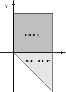
Figure 1: Mean-field phase diagram of a $p\,$-wave superconductor as described by Eq. (1). See the text for additional information.

III.2 Renormalized mean-field theory

A better approximation is to still treat the order parameter as a constant, ${\bm{\psi}}({\bm{x}})\equiv{\bm{\psi}}$, but to keep the electromagnetic fluctuations. The part of the action that depends on the vector potential then takes the form

$$S_{A}=\frac{1}{8\pi\mu}\int d{\bm{x}}\ \left[k_{\lambda}^{2}{\bm{A}}^{2}({\bm{x}})+\left({\bm{\nabla}}\times{\bm{A}}({\bm{x}})\right)\right],$$ (7a)

where

$$k_{\lambda}=(8\pi\mu cq^{2}|{\bm{\psi}}|^{2})^{1/2}$$ (7b)

is the inverse London penetration depth. Since ${\bm{A}}$ enters $S_{A}$ only quadratically, it can be integrated out exactly,gau and the technical development is identical to the $s$-wave case.Halperin et al. (1974); Chen et al. (1978) The result for the leading terms in powers of $|{\bm{\psi}}|^{2}$ in $d=3$ is

$$f=t\,|{\bm{\psi}}|^{2}+u\,|{\bm{\psi}}|^{4}-w\,(|{\bm{\psi}}|^{2})^{3/2}+v\,|{\bm{\psi}}\times{\bm{\psi}}^{*}|^{2}\ .$$ (8)

Here $w\propto\sqrt{\mu q^{2}}$ is a positive coupling constant whose presence drives the transition into either of the ordered phases first order.

There are several interesting aspects of this result. First, the additional term in the mean-field free energy, with coupling constant $w$, is not analytic in $|{\bm{\psi}}|^{2}$. This is a result of integrating out the vector potential, which is a soft or massless fluctuation. Second, the resulting first-order transition is an example of what is known as the Coleman-Weinberg mechanism in particle physics,Coleman and Weinberg (1973) or a fluctuation-induced first-order transition in statistical mechanics.Halperin et al. (1974)

Let us discuss the validity of the renormalized mean-field theory. The length scale given by the London penetration depth $\lambda=k_{\lambda}^{-1}$ needs to be compared with the second length scale that characterizes the action, Eq. (1), which is the superconducting coherence length $\xi=\sqrt{c/|t|}$. The ratio $\kappa=\lambda/\xi$ is the Landau-Ginzburg parameter. For $\kappa\to 0$, order parameter fluctuations are negligible (this is the limit of an extreme type-I superconductor), and the renormalized mean-field theory become exact. For nonzero values of $\kappa$ the fluctuations of the order parameter cannot be neglected, and the question arises whether or not they change the first-order nature of the transition. We will investigate this question next by means of two different technical approaches.

III.3 $\epsilon$-expansion about $d=4$

We first perform a momentum-shell renormalization-group (RG) analysis of the action, Eq. (LABEL:eq:2.3), in $d=4-\epsilon$ dimensions. The propagators can be read off the action, Eq. (LABEL:eq:2.3). For the $\psi$-propagator we have

$$\langle\psi_{\alpha}({\bm{k}})\,\psi^{*}_{\beta}(-{\bm{k}})\rangle=\frac{\delta_{\alpha\beta}}{t+ck^{2}}\ .$$ (9a)

In Coulomb gauge, $${\bm{\nabla}}\cdot{\bm{A}}=0$$, one finds for the gauge field propagator

$$\langle A_{i}({\bm{k}})\,A_{j}(-{\bm{k}})\rangle=4\pi\mu\,\frac{\delta_{ij}-{\hat{k}}_{i}{\hat{k}}_{j}}{k^{2}}\ ,$$ (9b)

where ${\hat{k}}_{i}$ denotes the components of the unit vector ${\hat{\bm{k}}}={\bm{k}}/k$. $\langle\ldots\rangle$ denotes an average with respect to the Gaussian part of the action, Eq. (LABEL:eq:2.3). The vertices as given by the action, Eq. (LABEL:eq:2.3), are shown graphically in Fig. 2,

Figure 2: Interaction vertices as given by the action, Eq. (LABEL:eq:2.3). Solid and dashed lines denote the electron fields ${\bm{\psi}}$ and ${\bm{\psi}}^{*}$, respectively, and wavy lines denote the gauge field ${\bm{A}}$. The dotted lines serve to separate different components of the electron fields.

and the one-loop diagrams that renormalize the various coupling constants in the action are shown in Fig. 3.

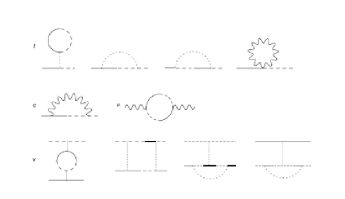
Figure 3: One-loop diagrams that renormalize the coupling constants $t$, $c$, $u$, $v$, $q$, and $\mu$ in Eq. (LABEL:eq:2.3).

The calculation is now a straightforward generalization of the one for the s-wave case, Ref. Halperin et al., 1974. We define the scale dimension of a length $L$ to be $[L]=-1$, and exponents $\eta$ and $\eta_{A}$ by choosing the scale dimensions of the fields ${\bm{\psi}}$ and ${\bm{A}}$ to be $[{\bm{\psi}}({\bm{x}})]=(d-2+\eta)/2$ and $[{\bm{A}}({\bm{x}})]=(d-2+\eta_{A})/2$, respectively. We find RG recursion relations

$$\frac{dt}{dl} = (2-\eta)\,t+3\,c\,q^{2}\mu+\frac{(n+2)u+4v}{t+c}\ ,$$ (10a)

$$\frac{du}{dl} = (\epsilon-2\eta)\,u-\frac{(n+8)u^{2}+8uv+8v^{2}}{(t+c)^{2}}-3\,c^{2}q^{4}\mu^{2},$$

(10b)

$$\frac{dv}{dl} = (\epsilon-2\eta)\,v-\frac{nv^{2}+12uv}{(t+c)^{2}}\ ,$$ (10c)

$$\frac{dc}{dl} = -\eta\,c-3\frac{c^{2}q^{2}\mu}{t+c}\ ,$$ (10d)

$$\frac{d\mu}{dl} = \eta_{A}\,\mu-\frac{n}{6}\,\frac{(3t+c)c^{3}q^{2}\mu^{2}}{(t+c)^{4}}\ ,$$ (10e)

$$\frac{dq}{dl} = \frac{1}{2}\,(\epsilon-\eta_{A})\,q.$$ (10f)

Here $l=\ln b$ with $b$ the length rescaling parameter, we have redefined $4\pi\mu\to\mu$, and we have absorbed a common geometric factor in the coupling constants $u$, $v$, and $\mu$. For $v=0$, these flow equations reduce to those of Ref. Halperin et al., 1974, as they should.

We now look for fixed points (FPs) of the Eqs. (10). Since we are interested in superconductors (as opposed to superfluids), we are looking for a FP where the charge is nonzero. Equation (10f) immediately yields

$$\eta_{A}=\epsilon.$$ (11a)

Anticipating a FP value $$t^{*} t O(\epsilon) (q^{2}\mu)^{*}=6\epsilon/n+O(\epsilon^{2}) \eta c$$ of that is of , Eq. (10e) then implies . If we choose such that is not renormalized, Eq. (10d) in turn yields

$$\eta=-18\epsilon/n+O(\epsilon^{2}).$$ (11b)

We now look for FP values of $u$ and $v$ that are of $O(\epsilon)$. Equation (10a) then indeed yields $t^{*}=O(\epsilon)$, so the remaining task is to consider Eqs. (10b, 10c). Let us define $x=u^{*}/\epsilon c^{2}$ and $y=v^{*}/\epsilon c^{2}$. The remaining FP equations then read

$$(n+8)x^{2}+8xy+8y^{2}-\left(1+\frac{36}{n}\right)x+\frac{108}{n^{2}} = 0,$$

$$ny^{2}+12xy-\left(1+\frac{36}{n}\right)y = 0.$$

This set of two coupled quadratic equations has four solutions. Two of these are given by

$$y=0,$$ (13a)

and $$x$$ a solution of

$$(n+8)x^{2}-\left(1+\frac{36}{n}\right)x+\frac{108}{n^{2}}=0.$$ (13b)

Equation (13b) is the same condition as in the s-wave case, Ref.  Halperin et al., 1974. It has a real positive solution for $n>n_{\text{c}}^{\text{s}}\approx 365.9$. In this case, $v_{0}^{*}=0$, and $u_{0}^{*}=c^{2}x\epsilon+O(\epsilon^{2})>0$. We will refer to these as the s-wave FPs. The only other real solutions of Eq. (13b) occur in the unphysical region $n\lesssim-5.9$.

For $y\neq 0$, we have

$$x=\frac{1}{12}\left(1+\frac{36}{n}-ny\right),$$ (14a)

and $$y$$ a solution of

$$\hskip-20.0ptn^{2}(n^{3}+8n^{2}-96n+1152)y^{2}$$

$$\hskip 0.0pt-2n(n^{3}+38n^{2}+24n-1728)y$$

$$\hskip 0.0pt+(n^{3}+68n^{2}+1008n+10368)=0.$$ (14b)

For positive values of $n$, this equation has real solutions only for $n>n_{\text{c}}^{\text{p}}\approx 420.9$, which leads to two FPs that we refer to as the p-wave FPs. A stability analysis shows that of the four FPs found, the only stable one is the p-wave FP with the larger value of $y$. Linearizing about his FP yields the critical exponent $\nu$ for the corresponding continuous phase transition. For general $n$, the expression is very complicated. In the limit of large $n$, one finds

$$1/\nu=2-(1-1/n+O(1/n^{2}))\epsilon+O(\epsilon^{2}).$$ (15)

We conclude that for large $n$, and close to $d=4$, the phase transition in p-wave superconductors is continuous, as it is in the s-wave case, and that the p-wave case is in a different universality class. The analysis also suggests that for physical parameter values, $n=6$ and $d=3$, the transition is unlikely to be continuous. Of course, the same caveats as in the s-wave case apply with respect to the interpretation of this result. As was shown in Ref. Halperin et al., 1974, additional information can be obtained by means of an expansion in $1/n$ in $d=3$, and we perform such an analysis in the next subsection.

III.4 $1/n$-expansion in $d=3$

The technique of the $1/n$ expansion in a fixed dimension was developed by MaMa (1973) for an neutral $n$-component vector field, and it was generalized to the presence of a gauge field in Ref. Halperin et al., 1974. The basic idea is as follows. Consider the fully dressed or renormalized counterpart $G$ of the Gaussian propagator given in Eq. (9a). Its inverse can be written in terms of a self energy $\Sigma$,

$$G^{-1}(t,k)=t+ck^{2}+\Sigma(t,k).$$ (16)

At zero wave number, we have

$$G^{-1}(t,0)=t+\Sigma(t,0)\equiv t_{\text{R}},$$ (17a)

where $$t_{\text{R}} t t t_{\text{c}}$$ is the renormalized counterpart of . For approaching its critical value , it vanishes according to a power law

$$t_{\text{R}}\propto(t-t_{\text{c}})^{\gamma},$$ (17b)

characterized by the critical exponent $\gamma$. This implies $t_{\text{c}}=-\Sigma(t=t_{\text{c}},0)=-\Sigma(t_{\text{R}}=0,0)$, which allows to determine $t_{\text{c}}$ order by order in some perturbative scheme. At criticality, Eq. (16) can thus be rewritten

$$G^{-1}(t=t_{\text{c}},k) = ck^{2}+\Sigma(t=t_{\text{c}},k)-\Sigma(t=t_{\text{c}},0)$$

$$\propto k^{2-\eta}=k^{2}\left[1-\eta\ln k+O(\eta^{2})\right],$$

(18)

with the critical exponent $\eta$. Now consider a perturbative expansion for $\Sigma$ with $1/n$ as the small parameter. Assuming that $\eta$ is small, it thus can be determined perturbatively from the wave number dependence of $\Sigma(t=t_{\text{c}},k)-\Sigma(t=t_{\text{c}},0)$. To zeroth order in this expansion, there is no contribution, so $G^{-1}(t=t_{\text{c}},k)\propto k^{2}$, and $\eta=0$. To first order in $1/n$, there is a contribution, as one would expect from the result of the $\epsilon$ expansion, Eq. (11b).

Similarly, $\gamma$ can be obtained perturbatively from the behavior of the self energy at $k=0$. From Eqs. (16, 17) we have

$$t_{\text{R}}+\Sigma(t_{\text{R}}=0,0)-\Sigma(t_{\text{R}},0)=t-t_{\text{c}}\propto t_{\text{R}}^{1/\gamma}.$$ (19)

To zeroth order in $1/n$ one finds, in $d=3$, $\Sigma(t_{\text{R}}=0,0)-\Sigma(t_{\text{R}},0)\propto t_{\text{R}}^{1/2}$. That is, $\gamma=2$, which is result for the spherical model. If we write corrections to this result in terms of an exponent $\zeta$, $1/\gamma=1/2-\zeta$, we have

$$\Sigma(t_{\text{R}}=0,0)-\Sigma(t_{\text{R}},0)\propto t_{\text{R}}^{1/2-\zeta}=t_{\text{R}}^{1/2}[1-\zeta\ln t_{\text{R}}+O(\zeta^{2})].$$ (20)

$\zeta$ can just be obtained as the prefactor of a dependence of the self energy on $t_{\text{R}}^{1/2}\ln t_{\text{R}}$.

For s-wave superconductors, this calculation has been performed in Ref. Halperin et al., 1974. For the current problem, the calculation is straightforward. This calculation yields

$$\eta = \frac{-104}{3\pi^{2}}\,\frac{1}{n}+O(1/n^{2}),$$ (21a)

$$\gamma = 2\left(1-\frac{100}{\pi^{2}}\,\frac{1}{n}+O(1/n^{2})\right).$$ (21b)

All other static critical exponents can be obtained from these two by means of scaling relations. In particular, for the correlation length exponent $$\nu$$ we have

$$\nu=1-\frac{352}{3\pi^{2}}\,\frac{1}{n}+O(1/n^{2}).$$ (21c)

To this order, $\nu$ is positive for $n>352/3\pi^{2}\approx 11.9$, which suggests again that the transition is first order for the physical case $n=6$ in $d=3$.

IV Summary

In summary, we have considered the critical behavior of a p-wave superconductor in both an $\epsilon$ expansion about $d=4$, and in a $1/n$ expansion in $d=3$, in analogy to the analysis of s-wave superconductors in Ref. Halperin et al., 1974. We have found that the results are qualitatively the same: both methods suggest that, for physical parameter values, the superconducting transition is fluctuation-induced first order in nature. For a model with an $n$-component order parameter, the suppression of fluctuations for sufficiently large $n$ leads to a continuous transition that is in a different universality class than the corresponding transition in the s-wave case. To first order in $\epsilon=4-d$, the critical value of $n$ that separates the first-order and second-order cases is $n_{\text{c,p}}=420.9$ for the p-wave case, whereas in the s-wave case one has $n_{\text{c,s}}=365.9$. In a $1/n$ expansion in $d=3$, the critical $n$-value in the p-wave case is equal to $11.9$, compared to $9.72$ in the s-wave case. These values have to be compared to the physical values $n=2$ and $n=6$ in the s-wave and p-wave cases, respectively. The caveats related to critical fixed points that are not accessible by either perturbative method that have been discussed for the s-wave caseDasgupta and Halperin (1981); Bartholomew (1983) apply to the p-wave case as well.

V acknowledgments

This work was supported by the NSF under grant No. DMR-05-29966.

References

- Halperin et al. (1974) B. I. Halperin, T. C. Lubensky, and S.-K. Ma, Phys. Rev. Lett. 32, 292 (1974).
- Coleman and Weinberg (1973) S. Coleman and E. Weinberg, Phys. Rev. D 7, 1888 (1973).
- Nounesis et al. (1993) G. Nounesis, K. I. Blum, M. J. Young, C. W. Garland, and R. J. Birgeneau, Phys. Rev. E. 47, 1910 (1993).
- Dasgupta and Halperin (1981) C. Dasgupta and B. I. Halperin, Phys. Rev. Lett. 47, 1556 (1981).
- Bartholomew (1983) J. Bartholomew, Phys. Rev. B 28, 5378 (1983).
- Herbut and Tesanovic (1996) I. Herbut and Z. Tesanovic, Phys. Rev. Lett. 76, 4588 (1996).
- Herbut and Tesanovic (1997) I. Herbut and Z. Tesanovic, Phys. Rev. Lett. 78, 980 (1997).
- Nelson et al. (2004) K. D. Nelson, Z. Q. Mao, Y. Maeno, and Y. Liu, Science 306, 1151 (2004).
- Rice (2004) M. Rice, Science 306, 1142 (2004).
- Machida and Ohmi (2001) K. Machida and T. Ohmi, Phys. Rev. Lett. 86, 850 (2001).
- Vollhardt and Wölfle (1990) D. Vollhardt and P. Wölfle, The Superfluid Phases of Helium 3 (Taylor & Francis, 1990).
- Knigavko et al. (1999) A. Knigavko, B. Rosenstein, and Y. F. Chen, Phys. Rev. B 60, 550 (1999).
- (13) The -vertex as given by has a zero eigenvalue, and hence the -propagator does not exist. This problem, which reflects gauge invariance, is readily solved by adding a gauge fixing term to the action that enforces a particular choice of gauge, see, e.g., Ref. Ryder, 1985.
- Chen et al. (1978) J. H. Chen, T. C. Lubensky, and D. R. Nelson, Phys. Rev. B 17, 4274 (1978).
- Ma (1973) S.-K. Ma, Phys. Rev. A 7, 2172 (1973).
- Ryder (1985) L. H. Ryder, Quantum Field Theory (Cambridge University Press, Cambridge, 1985).