Controlling soliton interactions in Bose-Einstein condensates by synchronizing the Feshbach resonance and harmonic trap

Abstract

We present how to control interactions between solitons, either bright or dark, in Bose-Einstein condensates by synchronizing Feshbach resonance and harmonic trap. Our results show that as long as the scattering length is to be modulated in time via a changing magnetic field near the Feshbach resonance, and the harmonic trapping frequencies are also modulated in time, exact solutions of the one-dimensional nonlinear Schrödinger equation can be found in a general closed form, and interactions between two solitons are modulated in detail in currently experimental conditions. We also propose experimental protocols to observe the phenomena such as fusion, fission, warp, oscillation, elastic collision in future experiments.

I I. Introduction

Observation of Bose-Einstein condensates (BECs) in gases of weakly interacting alkali-metal atoms has stimulated intensive studies of the nonlinear matter waves. One of the central questions in this field is how to explore properties of BECs. It is known that interatomic interactions greatly affect a number of properties of BECs, including both static (such as the size, shape and stability) and dynamic ones (like the collective excitation, soliton, and vortex behavior, etc.). A common practice to change the interaction strength, even its sign, is to modulate the $s$-wave scattering length, $a_{s}$, by using the Feshbach resonance with a tunable time-dependent magnetic field $B(t)$ Moerdijk ; Roberts ; Stenger ; Inouye ; Cornish ; Donley ; Regal ; Volz03 : $a_{s}(t)=a_{\infty}[1-\triangle/(B(t)-B_{0})]$, where $a_{\infty}$ is the off-resonance scattering length, $t$ is the time, $B_{0}$ and $\triangle$ are the resonance position and width, respectively. This offers a good opportunity for manipulation of atomic matter waves and nonlinear excitations in BECs. In real experiments, various forms of the time dependence of $B(t)$ have been explored K. E. Strecker ; C. A. Regal ; M. Greiner , observation of dark and bright solitons have been reported. In theoretical studies, several forms of time-varying scattering lengths have been proposed and treated separately, such as the exponential function $e^{\lambda t}$ F. Kh. Abdullaev ; V. M. Perez-Garcia ; Z. X. Liang , or the periodic function $g_{0}+g_{1}\sin(\Omega t)$ H. Saito ; D. E. Pelinovsky ; G. D. Montesinos ; Konotop95 ; M. Matuszewski , and so on.

In the present paper, we will consider the general case with arbitrary, time-varying scattering length $a_{s}(t)$, and discuss how to control dynamics of solitons in BECs by synchronizing the Feshbach resonance and harmonic trap in current experimental conditions. We first obtain a family of exact solutions to the general nonlinear Schrödinger equation with an external potential and arbitrary time-varying scattering length $a_{s}(t)$, then further discuss how to control the interaction of solitons including the bright and dark solitons. We observe several interesting phenomena such as fusion, fission, warp, oscillation, elastic collision in BECs with different kinds of scattering length correspond to different real experimental cases.

II II. the model and soliton solutions

Consider condensates in a harmonic trap $V({\bf r})=m\omega^{2}_{\bot}(y^{2}+z^{2})/2+m\omega^{2}_{1}x^{2}/2$, where $m$ is atomic mass, $\omega_{\bot}$ and $\omega_{1}$ the transversal and axial frequency, respectively. Such a trap can be realized, for instance, as a dipole trap formed by a strong off-resonant laser field. In the mean-field theory, the dynamics of BEC at low temperature is governed by the so-called Gross-Pitaevskii (GP) equation in three-dimensions. If $\omega_{\bot}\gg|\omega_{1}|$, it is reasonable to reduce the GP equation for the condensate wave function to the quasi-one-dimensional (quasi-1D) nonlinear Schrödinger equation K. D. Moll ; G. Fibich ; Garcia98 ; Kevrekidis04 ; Brazhnyi04 ,

$$i\frac{\partial\psi}{\partial t}=-\frac{1}{2}\frac{\partial^{2}\psi}{\partial x^{2}}+\frac{a_{s}(t)}{a_{B}}|\psi|^{2}\psi+\frac{\omega^{2}_{1}}{2\omega^{2}_{\bot}}x^{2}\psi,$$ (1)

where the time $t$ and coordinate $x$ are measured, respectively, in units of $\omega^{-1}_{\bot}$ and $a_{\bot}$, with $a_{\bot}\equiv\sqrt{\hbar/m\omega_{\bot}}$; $\psi$ is measured in units of $1/(\sqrt{2\pi a^{2}_{\bot}a_{B}})$, with $a_{B}$ as the Bohr radius. The key observation of the present paper is that if we allow the axial frequency of the harmonic trap becomes also time dependent $\omega_{1}=\omega_{1}(t)$, and require it to satisfy the following integrability relation with the scattering length $a_{s}(t)$, we have

$$-\frac{1}{a_{s}(t)}\frac{d^{2}a_{s}(t)}{dt^{2}}+\frac{2}{a_{s}^{2}(t)}(\frac{da_{s}(t)}{dt})^{2}+\frac{\omega^{2}_{1}(t)}{\omega^{2}_{\bot}}=0.$$ (2)

Then, the nonlinear GP equation (1) with time-varying coefficients can be reduced to the standard nonlinear Schrödinger equation and exactly solved, with the following general solution:

$$\psi(x,t)=exp[-\int\limits^{t}_{t_{0}}\Gamma(t)dt]\phi(X,T)\exp[i\Gamma(t)x^{2}],$$ (3)

where $\phi$ is an arbitrary function of $X$ and $T$, with new spatial and temporal variables $X=A_{1}\exp[-2\int\limits^{t}_{t_{0}}\Gamma(t)dt]x$, $T=\frac{A^{2}_{1}}{2}\int\limits^{t}_{t_{0}}\exp[-4\int\limits^{t}_{t_{0}}\Gamma(t^{\prime})dt^{\prime}]dt$. $A_{1}$ is a real constant, which together with $\Gamma(t)$ are determined by

$$a_{s}(t)=\pm a_{B}A^{2}_{1}\exp[-2\int\limits^{t}_{t_{0}}\Gamma(t)dt].$$ (4)

Meanwhile, the trapping frequency can also be expressed in terms of $\Gamma(t)$ given by

$$\frac{\omega_{1}^{2}(t)}{\omega_{\bot}^{2}}=-2\Gamma_{t}-4\Gamma(t)^{2}.$$ (5)

From Eqs. (4) and (5), we see that both the scattering length and the trapping frequency can be expressed in terms of the $\Gamma$ function. It shows that the trapping potential can become repulsive, we will give a detailed exposition of this situation in the following section. Since the trapping potential we consider here is the cigar-shaped harmonic potential (here-after, the frequency $\omega_{\bot}$ is not varying), once the function of scattering length is determined, the $\Gamma$ function and the function of the trap potential can also be determined. Note that the exact solution $\psi(x,t)$ can be obtained for arbitrary time dependence of $a_{s}(t)$, since we can always choose an appropriate time-dependent axial frequency, $\omega_{1}(t)$, to satisfy the integrability relation.

When the interatomic interaction is attractive, i.e., $a_{s}(t)<0$, Eq. (1) has bright $N$-soliton solutions. The simplest case for studying soliton interactions is the two bright solitons solution, for which $\psi(x,t)$ is expressed by Eq. (3) with $\phi(X,T)$ given by

$$\begin{array}[]{ll}\phi(X,T)=2b\exp\{i[cX-(c^{2}-b^{2})T-\varphi]\}\times\\ \frac{(2b^{2}T-i)\cosh[b(X-2cT-X_{0})]+ib(X-2cT)\sinh[b(X-2cT-X_{0})]}{\cosh^{2}[b(X-2cT-X_{0})]+b^{2}[(X-2cT)^{2}+4b^{2}T]},\end{array}$$ (6)

where $b,c$, $\varphi$, $X_{0}$ are arbitrary constants.

When the interatomic interaction is repulsive, i.e., $a_{s}(t)>0$, there are dark $N$-soliton solutions to Eq. (1). For the two dark solitons solution, $\psi(x,t)$ is again expressed by Eq. (3), but with $\phi(X,T)$ given by

$$\phi(X,T)=\tau_{1}\exp\{i[l_{1}X-(l^{2}_{1}-2|\tau_{1}|^{2})T+\delta_{1}]\}\times$$

$$\frac{1+\epsilon[Z_{1}\exp(\xi_{1})+Z_{2}\exp(\xi_{2})]+\epsilon^{2}A_{12}Z_{1}Z_{2}\exp(\xi_{1}+\xi_{2})}{1+\epsilon[\exp(\xi_{1})+\exp(\xi_{2})]+\epsilon^{2}A_{12}\exp(\xi_{1}+\xi_{2})},$$ (7)

where $Z_{1}=(-\Omega_{1}+i\sqrt{4|\tau_{1}|^{2}-\Omega^{2}_{1}})/(\Omega_{1}+i\sqrt{4|\tau_{1}|^{2}-\Omega^{2}_{1}})$, $Z_{2}=(-\Omega_{2}+i\sqrt{4|\tau_{1}|^{2}-\Omega^{2}_{2}})/(\Omega_{2}+i\sqrt{4|\tau_{1}|^{2}-\Omega^{2}_{2}})$, $A_{12}=[(\Omega_{1}-\Omega_{2})^{2}+(\sqrt{4|\tau_{1}|^{2}-\Omega_{1}^{2}}-\sqrt{4|\tau_{1}|^{2}-\Omega_{2}^{2}})^{2}]/[(\Omega_{1}+\Omega_{2})^{2}+(\sqrt{4|\tau_{1}|^{2}-\Omega_{1}^{2}}-\sqrt{4|\tau_{1}|^{2}-\Omega_{2}^{2}})^{2}]$, $\xi_{1}=(\sqrt{4|\tau_{1}|^{2}-\Omega^{2}_{1}}-2l_{1})\Omega_{1}T+\Omega_{1}X+\xi^{(0)}_{1}$, $\xi_{2}=(\sqrt{4|\tau_{1}|^{2}-\Omega^{2}_{2}}-2l_{1})\Omega_{2}T+\Omega_{2}X+\xi^{(0)}_{2}$, $l_{1}$, $\delta_{1}$, $\Omega_{1}$, $\Omega_{2}$, $\xi^{(0)}_{1}$, $\xi^{(0)}_{2}$, $\epsilon$ are real constants, and $\tau_{1}$ is complex constants.

III III. effects of the time-dependent magnetic fields on the solitons

Now we consider the elementary applications of solutions (3) with (6) and (7) respectively, with linear, exponential and sinusoidal time dependence of the magnetic field via Feshbach resonance, and propose how to control dynamics of solitons in BECs by synchronizing Feshbach resonance and harmonic trap in future experiments.

IV A. Magnetic field ramped linearly with time

In real experiments Volz03 ; C. A. Regal , the magnetic field is linearly ramped down with time $t$. We can design an experimental protocol to control the soliton interaction in BECs near Feshbach resonance with the following steps: (i) In real experiment of ⁸⁷Rb atoms, the scattering length can be chosen as a function of magnetic field, i.e., $a_{s}(t)=a_{\infty}[1-\triangle/(B(t)-B_{0})]$ Volz03 , where the off-resonant scattering length $a_{\infty}=108a_{B}$, $a_{B}$ is the Bohr radius, $B_{0}$ is the Feshbach resonance position, and $\triangle$ is the resonance width, respectively. The best-fit value for the width is $\triangle=0.20$ G, resulting in $B_{0}=1007.40$ G. Near the Feshbach resonance, the field $B(t)$ varies linearly with the rate 0.02 G/ms. For a better understanding, we plot Fig. 1, which shows the scattering length and the trapping frequency vary with time when the field $B(t)$ approaches the Feshbach resonance position $B_{0}$. (ii) The realistic experimental parameters for a quasi-1D repulsive condensate can be chosen $N\sim 10^{3}$ atoms and with peak atomic density $n_{0}=10^{5}cm^{-1}$. Then the scattering length $a_{s}$ is of order of nanometer, e.g., $|a_{s}|=5.8$ nm for a ⁸⁷Rb condensate, and $\omega_{\bot}=2\pi\times 400$ Hz, with the ratio $\omega_{1}/\omega_{\bot}$ being very close to zero.

The validity of the GP equation relies on the condition that the system be dilute and weakly interacting: $n|a_{s}|^{3}\ll 1$, where $n$ is the average density of the condensate. Applying the above conclusions to real experiments, we need to examine whether the validity condition for the GP equation can be satisfied or not. In the ground state for ⁸⁷Rb condensate, the scattering length is known to be $|a_{s}|=5.8$ nm Volz03 ; the typical value of the density ranges from $10^{13}-10^{15}$ cm^-3. So $n|a_{s}|^{3}<10^{-3}\ll 1$ is satisfied. Moreover, the experimental data agree reasonably well with the mean-field results D. S. Jin , which further proves the validity of the GP equation with $|a_{s}|=5.8$nm. Another important issue is quantum depletion of the condensate, which is ignored in the derivation of the GP equation. The physics beyond the GP equation should also be very rich, and we will work on more rigorous solutions beyond the GP equation in the future.

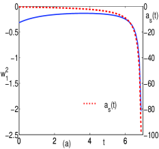
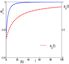
Figure 1: (color online) The scattering length (red dotted line) and the trapping potential (blue solid line) vary with time when the magnetic field ramps linearly with time $t$. (a) The selected field $B(t)$ varies from 1007.54 G to 1007.42 G, corresponding to the attractive interaction between atoms. (b) The selected field $B(t)$ varies from 1007.70 G to 1008.50 G, corresponding to the repulsive interaction between atoms. The scattering length is measured in units of $a_{\infty}$, the axial frequency is measured in units of $w_{\bot}^{2}$, and the field $B(t)$ varies linearly with the rate 0.02 G/ms.

Figure 2(a) shows the bright solitons interaction in BECs near the Feshbach resonance. In this case, the $s$-wave scattering length $a_{s}<0$. According to the integrability relation, the time-dependent axial frequency is imaginary which indicates a repulsive potential. As shown in Fig. 1(a), when the field $B(t)$ approaches the Feshbach resonance position $B_{0}$, the absolute value of the scattering length increases, but the time-dependent axial frequency decrease linearly. With the increasing of the absolute of the scattering length, the interactions between atoms become stronger, the peak of each soliton increases and its width decreases. Meanwhile, under the expulsive potential, the two bright solitons will be set into motion. As a result, the left bright soliton feels two forces which come from the right bright soliton and the trapping potential, it drives the left bright soliton to the right-hand side. The right-hand one moves slower than the left-hand one. Finally, the distance between the solitons becomes smaller. When the field $B(t)$ infinitely approaches $B_{0}$, the absolute value of the scattering length and axial frequency become infinite. The two solitons interact very strongly and almost merge into one with a very high peak and the narrowest width. After at least close to 1007.50 G, the absolute value of the atomic scattering length becomes $|a_{s}(t)|=5.7$ nm $<5.8$ nm for quasi-1D ⁸⁷Rb gas mentioned above. This means that the stability of soliton and the validity of 1D approximation is maintained from 1007.54 G to 1007.50 G. With further increasing of $|a_{s}|$ [for example, while $B(t)=1007.46$G, $|a_{s}|$ should be $13.3$nm], the system may be beyond the validity of the GP equation. Therefore, the phenomena discussed in Fig. 2(a) should be observable within the current experimental condition from 1007.54 G to 1007.50 G. With synchronized Feshbach resonance and harmonic trap to change the scattering length and axial frequency, we can easily control matter wave soliton interactions and obtain a new type of atom laser with manipulatable intensity.

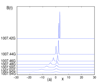
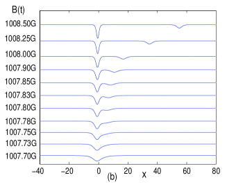
Figure 2: (color online) Controlling matter wave bright and dark soliton interaction near the Feshbach resonance ($B_{0}=1007.40$ G) when the magnetic field ramps linearly with time $t$. (a) The selected field $B(t)$ varies from 1007.54 G to 1007.42 G. The parameters are given as follows: $b=0.01$, $X_{0}=3000$, $c=0.002$ in Eq. (3) with Eq. (6). (b) The selected field $B(t)$ varies from 1007.70 G to 1008.50 G. The parameters are given as follows: $|\tau_{1}|^{2}=0.0001$, $\Omega_{1}=0.01$, $\Omega_{2}=-0.02$, $\xi^{(0)}_{1}=112$, $\xi^{(0)}_{2}=0$, $\epsilon=1$ in Eq. (3) with Eq. (7).

Figure 2(b) shows the interaction of dark solitons with magnetic field being selected in the range from 1007.70 G to 1008.50 G. In this case, as shown in Fig. 1(b), the $s$-wave scattering length $a_{s}>0$, and is in proportion to the magnetic field, the axial time-dependent decrease linearly and asymptotic approaches to zero, it means that the system becomes a self-confined condensate. Initially, there is only one dark soliton in BECs. Repulsive interaction between atoms becomes stronger when the absolute value of $a_{s}$ increases. This causes the dark soliton to split and finally become two dark solitons, meanwhile, each soliton increases its peak and compresses its width. However, contrary to the bright soliton shown in Fig. 2(a), one dark soliton moves away from the other. After at least close to 1008.50 G, the absolute value of the atomic scattering length becomes $|a_{s}(t)|=4.67$ nm, which is safely smaller than 5.8 nm for quasi-1D ⁸⁷Rb condensate, thus the stability of the soliton and validity of the 1D approximation are maintained. We conclude that the dark soliton fission phenomenon revealed here can be realized under the current experimental condition.

V B. magnetic field varying exponentially with time

When the field is exponentially ramped down as $\exp(-t/\tau)$ to a selected field between 545 G and 630 G K. E. Strecker , where $\tau=40$ ms, $a_{s}$ small and negative or small and positive, the interaction parameter $g(t)$ near the resonance varies exponentially with time: $g(t)\equiv a_{s}/a_{B}=\pm 0.01\exp(\lambda t)$, where $\lambda=|\omega_{1}|/\omega_{\bot}\ll 1$. The integrability relation reads $-\lambda^{2}=\frac{w_{1}^{2}}{w_{\bot}{2}}$, and can be satisfied automatically as long as the time-dependent axial frequency is imaginary which indicates a repulsive trapping potential. With the same parameters as in the experiment L. Khaykovich , i.e., $N\approx 10^{3}$, $\omega_{\bot}=2\pi\times 700$ Hz, $\omega_{1}=2i\pi\times 21$ Hz, and $\lambda=0.03$, the interactions between the two bright solitons is shown in Fig. 3. It is interesting to observe that in the expulsive parabolic potential, the bright solitons are set into motion and propagate in the axial direction. With time going on, $|a_{s}(t)|$ increases. We could observe an increase in their peaking values and a compression in widths, besides that the spacing between them decreases after they are initially generated on different positions in the trap, which is evidence for a short-range attractive interaction between solitons. Finally, they almost merge and fusion. This phenomena is different from the case of K. E. Strecker ; L. Khaykovich . There, the bright solitons are set in motion by off setting the optical potential and propagate in the potential for many oscillatory cycles with the period 310 ms, the spacing between the solitons increase near the center of oscillation and bunches at the end points. The difference is mainly caused by two factors: one is the time-varying scattering length strongly affect the interaction between the solitons, and the other reason is the repulsive force provided by the potential. Meanwhile, with the increasing of the scattering length, the attractive interaction between atoms become stronger, this will leads to an attractive interaction between solitons. Eventually, the outcome of these two forces will determine the motion of the two bright solitons.

Fusion is very interesting phenomenon and it comes from the interatomic attractive interaction. In other words, with time going on, both bright solitons change their positions, warp in a certain radian, and almost merge into one single soliton. Such morphology has been observed in coronal plasma L. Golub . We hope that such morphology would be detected in BEC experiments too in the near future.

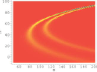
Figure 3: (color online) Controlling matter wave bright soliton interaction when field varying exponentially with time. The parameters are given as follows: $\lambda=0.03$, $b=0.5$, $X_{0}=20$, $c=7$ in Eq. (3) with Eq. (6). The color corresponds to the BEC density, with yellow (gray) being the smallest and blue (dark) being the largest.

In real experiments K. E. Strecker , the length of the background of BECs can reach at least $2L=370$ $\mu$m. At the same time, in Fig. 3, solitons travel from $x=$ 50 to 200, i.e., $150\times 1.4$ $\mu$m$=210$ $\mu$m. [The dimensionless unit of the coordinate, $\Delta x=1$, corresponds to $a_{\bot}=(\hbar/m\omega_{\bot})^{1/2}=1.4$ $\mu$m]. We indeed have $210$ $\mu$m $<370$ $\mu$m, a necessary condition for observing the morphology in BEC experiments Z. X. Liang . Additionally, after at least up to 100 dimensionless units of time, $|a_{s}(t)|$ reaches the value $0.2a_{B}$, which is less than $|a_{final}|=4a_{B}$. This means that during the time evolution, the stability of solitons and the validity of 1D approximation can be maintained as displayed in Fig. 3. Therefore, the phenomena discussed in this case are also expected to be observable within the current experimental capability.

The interactions between two dark solitons are also intriguing. The first experimental evidence of attraction between dark solitons in nonlocal nonlinear media has been presented A. Dreischuh . Our results (3), (5), and (7) also indicated that attraction between dark solitons should be observable in BECs with repulsive long-range interatomic interaction. In a previous case, the field is linearly ramped down as time, leading to the trap axial frequency $\omega_{1}\cong 0$ and external potential vanishing. It means that the system becomes a self-confined condensate. So the repulsion between the dark solitons is observed in BEC with repulsive interatomic interaction [seen in Fig. 2(b)]. However, in the present case, the field varies exponentially with time, the trap axial potential is not vanishing and time independent, the system is in an expulsive parabolic potential. Following the experimental setup in L. Khaykovich , we can first create a BEC in the quasi-one-dimensional potential. Second, the trap potential is tuned to the value in our paper, meanwhile, the scattering length varies exponentially with time to a small and positive value. The potential provides an attractive force which counters the natural repulsion of the solitons. Finally, the competition between these two forces will determine the outcome of the interaction between solitons. If the attractive force which is caused by the potential is stronger than the natural repulsion of the solitons, the two dark solitons will move towards the other, which is the evidence for a short-range attractive interaction between dark solitons. However, the lifetime of a BEC in current experiments is of the order of 1 s and the region of a BEC is small, the solitons will be dissipation in their motion before reaching the edge of the condensate.

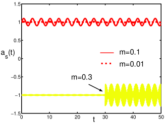
Figure 4: (color online) The scattering length varies with time when field varying periodically with time $t$. The yellow curve (gray) denotes the attractive interaction case, at $t=30$ (marked by an arrow), the amplitude of the scattering length is larger than before by suddenly jumping the amplitude of the ac drive $m$ to $m=0.3$, $w=30$. The red curve denotes the repulsive interaction for $m=0.1$ (dark solid line) and $m=0.01$ (dark dotted line), $w=2$. All of the lengths are measured in units of $a_{B}$.

VI C. magnetic field varying periodically with time

It was observed that a small sinusoidal modulation of the magnetic field close to the Feshbach resonance gave rise to a modulation of the interaction strength, $g(t)\equiv a_{s}(t)/a_{B}=\pm[1+m\sin(\omega t)]$ M. Greiner , where the amplitude $m$ of the ac drive was small and satisfied $0<m<1$. According to the integrability condition, the axial frequency of the harmonic potential should be

$$\omega^{2}_{1}(t)=-\frac{m\omega^{2}\omega^{2}_{\bot}}{[1+m\sin(\omega t)]^{2}}[\sin(\omega t)+m+m\cos^{2}(\omega t)].$$ (8)

Now, we investigate how the amplitude of the ac drive can be used to control the bright soliton interactions. As shown in Fig. 6, for the case with atomic attractive interaction, when the amplitude is small, $m=0.01$ ($0<t<30$). The periodically varying of the scattering length and the trapping frequency are small as shown in Figs. 4 and 5, the repulsive and attractive force between solitons can become balanced. Two bright solitons will move in parallel with their separation keeping constant. This property would be interesting for optical communication with low bit-error rates. In BEC, this effect may play an important role in potential application of matter wave communication with atom lasers. If the amplitude is increased to the value $m=0.3$ ($30<t<50$), the solitons begin to oscillate due to the temporal periodic modulation of the $s$-wave scattering and trapping potential are both stronger than before. This phenomena is very similar to the evolution of optical solitons.

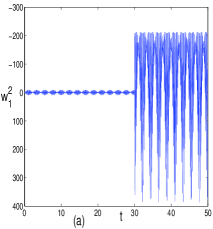
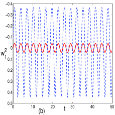
Figure 5: (color online) The trapping frequency varies with time when field varying periodically with time $t$. (a) $m=0.01$ ($0<t<30$), $m=0.3$ ($30<t<50$), and $w=30$ for the case with atomic attractive interaction. (b) $m=0.01$ (red solid line), $m=0.1$ (blue dashed line), and $w=2$ for the case with atomic repulsive interaction. The frequency is measured in units of $w_{\bot}^{2}$.

We also studied the effect of ac drive on interactions between the dark solitons. First, the amplitude $m$ of the ac drive is chosen small, $m=0.01$, this leads to a small periodical modulation of the scattering length and the trapping frequency. The repulsive interaction between atoms mainly leads to the formation of the dark solitons, this force cannot lead to a oscillation of the dark solitons due to the small change in the scattering length. As shown in Fig. 7(a), a faster soliton is generated behind a slower one in the mutual moving direction, after an interval of time, the faster one pulls up to the slower one and their elastic collision happens. After the collision, the faster one passes through the slower one and their parameters did not change, which remarkably indicates no energy exchange between the two dark solitons. For larger ac drive, for example, $m=0.1$, which is 10 times of the value of the previous $m$, with the same initial condition, because of the stronger modulation of the scattering length and the trapping frequency, both solitons move forward, meanwhile, they will oscillate back and forth, as shown in Fig. 7(b). In all of the above cases, the trap potential can become repulsive during the entire process, but the attractive potential is stronger than the repulsive one during a period, the outcome of the potential is an attractive one which can be seen in Fig. 5. It shows that a BEC with repulsive interaction between atoms is confined in the trap, this is different from the case B.

Another important problem is the atom loss. As the external magnetic field is driven close to the resonant value, the rate of loss of atoms is increasing rapidly in the vicinity of the Feshbach resonance, while only a small fraction of atoms remain as soliton. In all of the above cases, the scattering length is small, the validity of the GP equation is satisfied. Meanwhile, when the trapping potential is modulated according to the integrability relation, both the rate of the untrapped atom and the collective excitations will be further discussed.

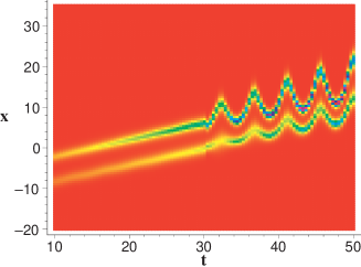
Figure 6: (color online) Controlling matter wave bright soliton interaction when field varying periodically with time, where (a) $m=0.01$ ($0<t<30$), (b) $m=0.3$ ($30<t<50$). The other parameters are as follows: $\omega=30$, $b=1$, $X_{0}=-9$, $c=0.4$ in Eq. (3) with Eq. (6).

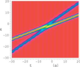
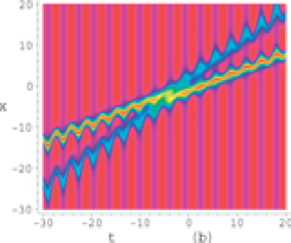
Figure 7: (color online) Controlling matter wave dark soliton interaction when field varying periodically with time, where (a) $m=0.01$, (b) $m=0.1$. The other parameters are as follows: $\omega=2$, $|\tau_{1}|^{2}=1$, $\Omega_{1}=1.2$, $\Omega_{2}=-1.8$, $l_{1}=0.02$, $\xi^{(0)}_{1}=-0.01$, $\xi^{(0)}_{2}=-0.2$, $\epsilon=1$ in Eq. (3) with Eq. (7).The red (with smaller slope) and blue correspond to the slower one and the faster one respectively.

VII IV. conclusion

In summary, we express how to control soliton interaction in BECs with arbitrary time-varying scattering length in a synchronized time-dependent harmonic trap. When the integrability condition is satisfied, we obtained the exact solutions analytically, and explored the interaction of the bright and dark solitons in BECs with Feshbach resonance magnetic field linearly, exponentially, and periodically dependent on time. In these typical examples, we find several interesting phenomena involving soliton interactions, such as fusion, fission, warp, oscillation, elastic collision, etc. F. K. Abdullaev ; G. Theocharis . We further discussed how to control interactions between bright or dark solitons, in BECs in realistic situations, which allows for experimental test of our predictions in the future. These phenomena open possibilities for future applications in coherent atom optics, atom interferometry, and atom transport.

This work was supported by NSFC Grants Nos. 90406017, 60525417 and 10740420252 and NKBRSFC Grants Nos. 2005CB724508 and 2006CB921400.

References

- (1) A. J. Moerdijk, B. J. Verhaar, and A. Axelsson, Phys. Rev. A 51, 4852 (1995).
- (2) J. L. Roberts, N. R. Claussen, James P. Burke, Jr., C. H. Greene, E. A. Cornell, and C. E. Wieman, Phys. Rev. Lett. 81, 5109 (1998).
- (3) J. Stenger, S. Inouye, M. R. Andrews, H. -J. Miesner, D. M. Stamper-Kurn, and W. Ketterle, Phys. Rev. Lett. 82, 2422 (1999).
- (4) S. Inouye, M. R. Andrews, J. Stenger, H. -J. Miesner, D. M. Stamper-Kurn, and W. Ketterle, Nature (london) 392, 151 (1998).
- (5) S. L. Cornish, N. R. Claussen, J. L. Roberts, E. A. Cornell, and C. E. Wieman, Phys. Rev. Lett. 85, 1795 (2000).
- (6) E. A. Donley, N. R. Claussen, S. L. Cornish, J. L. Roberts, E. A. Cornell, and C. E. Wieman, Nature (London) 412, 295 (2001).
- (7) C. A. Regal, and D. S. Jin, Phys. Rev. Lett. 90, 230404 (2003).
- (8) T. Volz, S. Drr, S. Ernst, A. Marte, and G. Rempe, Phys. Rev. A 68, 010702(R) (2003).
- (9) K. E. Strecker, G. B. Partridge, A. G. Truscoff, and R. G. Hulet, Nature (London) 417, 150 (2002).
- (10) C. A. Regal, M. Greiner, and D. S. Jin, Phys. Rev. Lett. 92, 040403 (2004).
- (11) M. Greiner, C. A. Regal, and D. S. Jin, Phys. Rev. Lett. 94, 070403 (2005).
- (12) F. K. Abdullaev, A. M. Kamchatnov, V. V. Konotop, and V. A. Brazhnyi, Phys. Rev. Lett. 90, 230402 (2003).
- (13) V. M. Pérez-García, V. V. Konotop, and V. A. Brazhnyi, Phys. Rev. Lett. 92, 220403 (2004).
- (14) Z. X. Liang, Z. D. Zhang, and W. M. Liu, Phys. Rev. Lett. 94, 050402 (2005).
- (15) H. Saito, and M. Ueda, Phys. Rev. Lett. 90, 040403 (2003).
- (16) D. E. Pelinovsky, P. G. Kevrekidis, and D. J. Frantzeskakis, Phys. Rev. Lett. 91, 240201 (2003).
- (17) G. D. Montesinos, V. M. Perez-Garcia, and H. Michinel, Phys. Rev. Lett. 92, 133901 (2004).
- (18) V. V. Konotop, and P. Pacciani, Phys. Rev. Lett. 94, 240405 (2005).
- (19) M. Matuszewski, E. Infeld, B. A. Malomed, and M. Trippenbach, Phys. Rev. Lett. 95, 050403 (2005).
- (20) K. D. Moll, A. L. Gaeta, and G. Fibich, Phys. Rev. Lett. 90, 203902 (2003).
- (21) G. Fibich, B. Ilan, and S. Schochet, Nonlinearity 16, 1809 (2003).
- (22) V. M. Pérez-García, H. Michinel, H. Herrero, Phys. Rev. A 57, 3837 (1998).
- (23) P. G. Kevrekidis and D. J. Frantzeskakis, Mod. Phys. Lett. B 18, 173 (2004).
- (24) V. A. Brazhnyi, and V. V. Konotop, Mod. Phys. Lett. B 18, 627 (2004).
- (25) D. S. Jin, J. R. Ensher, M. R. Matthews, C. E. Wieman, and E. A. Cornell, Phys. Rev. Lett. 77, 420 (1996).
- (26) L. Khaykovich, F. Schreck, G. Ferrari, T. Bourdel, J. Cubizolles, L. D. Carr, Y. Castin, and C. Salomon, Science 296, 1290 (2002).
- (27) L. Golub, J. Bookbinder, E. DeLuca, M. Karovska, and H. Warren, Phys. Plasmas 6, 2205 (1999).
- (28) A. Dreischuh, D. N. Neshev, D. E. Petersen, O. Bang, and W. Krolikowski, Phys. Rev. Lett. 96, 043901 (2006).
- (29) F. K. Abdullaev, and M. Salerno, J. Phys. B 36, 2851 (2003).
- (30) G. Theocharis, P. Schmelcher, P. G. Kevrekidis, and D. J. Frantzeskakis, Phys. Rev. A 72, 033614 (2005).