Optimizing the Double Description Method for
Normal Surface Enumeration

Abstract

Many key algorithms in 3-manifold topology involve the enumeration of normal surfaces, which is based upon the double description method for finding the vertices of a convex polytope. Typically we are only interested in a small subset of these vertices, thus opening the way for substantial optimization. Here we give an account of the vertex enumeration problem as it applies to normal surfaces, and present new optimizations that yield strong improvements in both running time and memory consumption. The resulting algorithms are tested using the freely available software package Regina.

AMS Classification 52B55 (57N10, 57N35)

1 Introduction

Some of the most fundamental problems in 3-manifold topology are algorithmic, such as determining the structure of a given space, or deciding whether two spaces are topologically equivalent. Much progress has been made on these problems; notable examples include the unknot recognition algorithm of Haken [13], the 3-sphere recognition algorithm of Rubinstein and Thompson [29, 30, 31], the connected sum and JSJ decomposition algorithms of Jaco and Tollefson [22], and the solution to the homeomorphism problem for Haken manifolds, developed by Haken [14] and completed by Jaco and Oertel [19] and Hemion [16].

Several recurring themes are found in these and many other topological algorithms: (i) they are extremely slow, (ii) they are extremely difficult to implement, and (iii) they are all based on normal surface theory.

The reason normal surface theory is so prevalent is because it allows topological existence problems to be converted into vertex enumeration problems on polytopes, which (being numerical and discrete) are far simpler to work with algorithmically.

Unfortunately this very technique that makes these problems approachable also makes the resulting algorithms impractically slow for all but the smallest 3-manifolds. This is because vertex enumeration can grow exponentially slow in the dimension of the polytope [11], which equates to exponentially slow in the complexity of the 3-manifold.

Any practical implementation therefore requires a highly optimized vertex enumeration algorithm. Vertex enumeration algorithms fall into two broad categories: those based on the double description method of Motzkin et al. [28], and those based on pivoting, as described for example by Dyer [11]. Both classes of algorithm have been analyzed and optimized in the literature; see for instance the optimized double description methods of Fukuda and Prodon [12], or the recent lexicographic pivoting method of Avis [1].

If we restrict our focus to topological problems, there are further gains to be had. Essentially, we can exploit the fact that normal surface algorithms typically require only a small number of polytope vertices, namely those that correspond to embedded surfaces in the underlying 3-manifold. We therefore have permission to ignore “most” of the vertices of the polytope, which opens the door to substantial improvements in efficiency.

The purpose of this paper is twofold. First we give a full description of the standard normal surface enumeration algorithm, which combines the double description method with the filtering method of Letscher—although well known, there is no account of this algorithm in the present literature. We then improve this algorithm by combining techniques from the literature with new ideas, cutting both running time and memory usage by orders of magnitude as a result.

We focus only on the double description method in this paper. Pivoting algorithms are certainly appealing, particularly because of their extremely low memory footprint [1, 3]. However, it is difficult to exploit the embedded surface constraints with these algorithms. We discuss this in more detail in Section 3.

On a practical note, there are two well-known implementations for the enumeration of normal surfaces: FXrays [9], by Culler and Dunfield, and Regina [4, 5], by the author. Both are freely available under the GNU General Public License. David Letscher wrote a proof-of-concept program Normal in 1999 that preceded both implementations, but his software is no longer available.

Each implementation has different design goals. FXrays uses highly streamlined code and data structures, and is very fast for the problems that it is designed for. Regina on the other hand is more failsafe and applicable to a wider range of problems, but pays a penalty in both time and memory usage. As an example, FXrays uses native integers where Regina uses arbitrary precision arithmetic, which makes FXrays faster and smaller but also at risk of integer overflow (which it detects but cannot overcome). Regina also uses slower filtering methods, but these generalize well to the sister problem of almost normal surface enumeration, which appears in some of the high-level topological algorithms mentioned earlier.

Since our concern here is the underlying algorithms, we focus on a single implementation (in this case, Regina). All of the improvements described here have been built into Regina version 4.5.1, released in October 2008, and it is pleasing to see that this new code enjoys significantly better time and memory performance than has been seen in either software package in the past.

The remainder of this paper is structured as follows. Section 2 begins with an outline of normal surface theory, focusing on its connections to polytope vertex enumeration. In Section 3 we describe the double description method, and explain how the filtering method of Letscher allows us to concentrate only on embedded surfaces. Section 4 presents a series of implementation techniques and algorithmic improvements that further optimize these core algorithms. These optimizations are put to the test in Section 5 with experimental measurements of running time and memory consumption, and Section 6 concludes with a summary of our findings.

The author is indebted to Bernard Blackham for his helpful suggestions regarding micro-optimization, and for highlighting the excellent references [10, 34] on this topic. Thanks must also go to the University of Melbourne for their continued support of the development of Regina.

2 Normal Surface Theory

Normal surfaces were introduced by Kneser [25], and further developed by Haken [13, 14] for use with the unknot recognition problem and the homeomorphism problem. They are now commonplace in recognition and decomposition algorithms, and more recently have found applications in simplification algorithms [20].

From a practical perspective, many of these algorithms are extremely messy and difficult to implement, due to the complex geometric operations involved and the myriad of problematic cases. Some have only recently been implemented in practice, such as the 3-sphere recognition and connected sum decomposition algorithms in Regina; others, such as JSJ decomposition or Haken’s homeomorphism algorithm, have never been implemented at all. Recent techniques have been developed to reduce both the difficulty and inefficiency of these algorithms; examples include Tollefson’s quadrilateral space [33], the crushing method of Jaco and Rubinstein [20], and the “guts” analysis of Jaco et al. [18].

Since the focus of this paper is on the double description method, we offer very little topological background, concentrating instead on the linear programming aspects of normal surface theory. For a more extensive review of normal surfaces, the reader is referred to [15] or [16].

2.1 Triangulations and Normal Surfaces

The key topological structures that we work with in this paper are triangulations and normal surfaces. We proceed to define each of these in turn.

Triangulations are representations of 3-manifolds that are ideal for computation. They are discrete structures, and they are very general—it is usually a simple matter to convert some other description of a 3-manifold (such as a Heegaard splitting or a Dehn filling) into a triangulation, whereas the other direction is often more difficult. Each of the high-level topological algorithms listed in the introduction takes a 3-manifold triangulation as input.

Definition 2.1 (Triangulation)

A 3-manifold triangulation of size $n$ is a finite collection of $n$ tetrahedra, where some or all of the $4n$ tetrahedron faces are affinely identified in pairs, and where the resulting topological space forms a 3-manifold. We allow identifications between different faces of the same tetrahedron, and likewise with edges and vertices. By a face, edge or vertex of the triangulation, we refer to an equivalence class of tetrahedron faces, edges or vertices under these identifications.

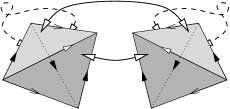
Figure 1: A two-tetrahedron triangulation of $S^{2}\times S^{1}$

As an example, Figure 1 shows a size two triangulation of the product space $S^{2}\times S^{1}$. In each tetrahedron the two rear faces are identified with a twist, and the two front faces of one tetrahedron are identified with the two front faces of the other. The triangulation only has one vertex (since all eight tetrahedron vertices are identified) and it has three distinct edges, indicated in the diagram by three different styles of arrowhead.

Normal surfaces are two-dimensional surfaces within a triangulation that intersect individual tetrahedra in a well-controlled fashion. These well-controlled intersections, defined in terms of normal discs, make it easier to analyze and search for surfaces that tell us about the topology of the underlying manifold.

Definition 2.2 (Normal Disc)

Let $\Delta$ be a tetrahedron in a 3-manifold triangulation. A normal disc in $\Delta$ is a topological disc embedded in $\Delta$ which does not touch any vertices of $\Delta$, whose interior lies in the interior of $\Delta$, and whose boundary consists of either (i) three arcs, running across the three faces surrounding some vertex, or (ii) four arcs, running across all four faces of the tetrahedron. Discs with three or four boundary arcs are called triangles or quadrilaterals respectively. Several normal discs are illustrated in Figure 2.

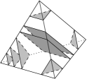
Figure 2: Normal discs inside a tetrahedron

There are seven different types of normal disc within a tetrahedron, defined by the choice of tetrahedron edges that a disc intersects. In particular, there are four triangle types (each meeting three edges) and three quadrilateral types (each meeting four edges), as illustrated in Figure 3.

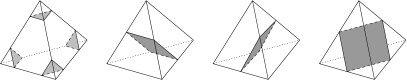
Figure 3: The seven different types of normal disc in a tetrahedron

Definition 2.3 (Normal Surface)

Let $\mathcal{T}$ be a 3-manifold triangulation. An embedded normal surface in $\mathcal{T}$ is a properly embedded surface in $\mathcal{T}$ that meets each tetrahedron in a collection of disjoint normal discs. Here we also allow disconnected surfaces (i.e., disjoint unions of smaller surfaces).

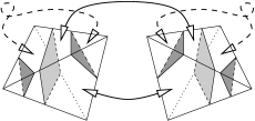
Figure 4: An embedded normal surface inside the triangulation of $S^{2}\times S^{1}$

To illustrate, Figure 4 shows an embedded normal surface inside the triangulation of $S^{2}\times S^{1}$ that was discussed earlier. The identifications of tetrahedron faces cause the six normal discs to join together to form a 2-sphere (which turns out to be a 2-sphere at one “level” of the product $S^{2}\times S^{1}$).

2.2 The Projective Solution Space

A key strength of normal surfaces is their ability to bridge the worlds of 3-manifold topology and linear algebra. We do this through the vector representation of a normal surface, which is defined below.

Throughout this section, we assume that $\mathcal{T}$ is a triangulation with $n$ tetrahedra, labelled $\Delta_{1},\ldots,\Delta_{n}$. For each tetrahedron, we arbitrarily number its triangular normal disc types $1,2,3,4$ and its quadrilateral normal disc types $1,2,3$.

Definition 2.4 (Vector Representation)

Let $S$ be an embedded normal surface within triangulation $\mathcal{T}$. For each tetrahedron $\Delta_{i}$, let $t_{i,j}$ be the number of triangular discs of the $j$th type contained in $S$ ($j=1,2,3,4$), and let $q_{i,k}$ be the number of quadrilateral discs of the $k$th type contained in $S$ ($k=1,2,3$). Then the vector representation of the surface $S$ is the $7n$-dimensional vector

$$(\ t_{1,1},t_{1,2},t_{1,3},t_{1,4},\ q_{1,1},q_{1,2},q_{1,3}\ ;\ t_{2,1},t_{2,2},t_{2,3},t_{2,4},\ q_{2,1},q_{2,2},q_{2,3}\ ;\ \ldots,q_{n,3}\ ).$$

Essentially the vector representation merely counts the number of normal discs of each type in each tetrahedron. As shown by Haken [13], this gives enough information to uniquely identify the surface, since there is only one way to glue the normal discs together without causing the surface to intersect itself:

Lemma 2.5

Let $S_{1}$ and $S_{2}$ be embedded normal surfaces in triangulation $\mathcal{T}$. If the vector representations of $S_{1}$ and $S_{2}$ are identical, then the surfaces $S_{1}$ and $S_{2}$ are ambient isotopic.

While every normal surface has a vector representation, there are of course $7n$-dimensional vectors that do not correspond to any embedded normal surface at all. It is therefore useful to pin down necessary and sufficient conditions on the vector representation.

Definition 2.6 (Admissible Vector)

Let $\mathbf{v}=(\ t_{1,1},t_{1,2},t_{1,3},t_{1,4},\ q_{1,1},q_{1,2},q_{1,3}\ ;\ \ldots,q_{n,3}\ )$ be a $7n$-dimensional vector of integers. This vector is admissible if it satisfies the following constraints:

• Non-negativity: Every coordinate of $\mathbf{v}$ is non-negative.

• Matching equations: Consider any two tetrahedron faces that are identified in the triangulation; suppose that the relevant tetrahedra are $\Delta_{i}$ and $\Delta_{j}$ (where $i=j$ is allowed). Let $F$ denote the resulting face of the triangulation, and let $e$ be any one of the three edges surrounding face $F$. We obtain an equation from $F$ and $e$ as follows.

  Precisely one of the four triangle types and one of the three quadrilateral types in each of $\Delta_{i}$ and $\Delta_{j}$ meets $F$ in arcs parallel to $e$. Let $t_{i,a}$, $q_{i,b}$, $t_{j,c}$ and $q_{j,d}$ be the corresponding coordinates of $\mathbf{v}$. Then it is true that $t_{i,a}+q_{i,b}=t_{j,c}+q_{j,d}$.

• Quadrilateral constraints: For each $i\in\{1,\ldots,n\}$, at most one of the coordinates $q_{i,1}$, $q_{i,2}$ and $q_{i,3}$ is non-zero.

It is straightforward to see that the vector representation of any embedded normal surface must be admissible:

• Non-negativity is clear because the vector representation counts discs.

• The matching equations express the fact that we must be able to glue together discs from adjacent tetrahedra. This is illustrated in Figure 5, where we see one triangle and one quadrilateral from $\Delta_{i}$ meeting two triangles from $\Delta_{j}$. The corresponding matching equation, derived from face $F$ and edge $e$, states that $t_{i,a}+q_{i,b}$ ($1+1$) equals $t_{j,c}+q_{j,d}$ ($2+0$).

  

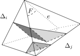
  Figure 5: The matching equations at work

• The quadrilateral constraints arise because any two quadrilaterals of different types in the same tetrahedron must intersect; this would make the resulting surface non-embedded.

A more interesting result of Haken [13] is that this implication works both ways:

Theorem 2.7

Let $\mathbf{v}$ be a $7n$-dimensional integer vector that is not the zero vector. Then $\mathbf{v}$ is the vector representation of an embedded normal surface in the triangulation $\mathcal{T}$ if and only if $\mathbf{v}$ is admissible.

It follows that, if we can characterize the non-negative solutions to the matching equations and the quadrilateral constraints, then we can completely characterize the space of embedded normal surfaces. That is, we can effectively convert topological questions into algebraic questions, granting us access to a wealth of knowledge in linear algebra and linear programming.

Definition 2.8 (Projective Solution Space)

Let $N\subseteq\mathbb{R}^{7n}$ be the set of vectors whose coordinates are non-negative and which satisfy the matching equations of Definition 2.6. Since the matching equations define a linear subspace of $\mathbb{R}^{7n}$, it follows that $N$ is a convex polyhedral cone with the origin as its vertex.

Let $P\subseteq N$ be the set of vectors in $N$ whose coordinates sum to one, that is, the intersection of the cone $N$ with the hyperplane $\sum t_{i,j}+\sum q_{i,k}=1$. Then $P$ is a (bounded) convex polytope in $\mathbb{R}^{7n}$, and is called the projective solution space for the original triangulation $\mathcal{T}$.

The importance of the projective solution space comes from the following observation: For many definitions of “interesting”, if a 3-manifold contains an interesting surface, then (with some rescaling) such a surface must appear at a vertex of the projective solution space. For instance, this is true of essential discs and spheres [22], and of two-sided incompressible surfaces [19]. This immediately yields an algorithm for testing whether an “interesting” surface exists:

• Enumerate the (finitely many) vertices of the projective solution space;

• For each vertex that satisfies the quadrilateral constraints, reconstruct the corresponding normal surface and test whether it is interesting.

This fundamental process sits at the core of every high-level topological algorithm described in the introduction, and many more besides.

As an implementation note, Tollefson [33] shows that in many scenarios the much smaller space $\mathbb{R}^{3n}$ can be used, where we define vectors that have only quadrilateral coordinates. The matching equations look different, but the overall procedure is much the same. The results presented in this paper apply equally well to both Tollefson’s quadrilateral space and the standard framework described above, and so we direct the reader to papers such as [20] or [33] for further details.

3 The Double Description Method

As described in the previous section, many high-level topological algorithms have at their core a polytope vertex enumeration procedure. Specifically, we must enumerate the vertices of the projective solution space. If we let $d$ denote the dimension of the surrounding vector space (so $d=7n$ in the framework of the previous section, or $3n$ in Tollefson’s quadrilateral space), then the projective solution space is a convex polytope formed by the intersection of:

• the non-negative orthant in $\mathbb{R}^{d}$, defined as $O=\{\mathbf{x}\in\mathbb{R}^{d}\,|\,x_{i}\geq 0\ \mbox{for all $i$}\}$;

• the projective hyperplane, defined as $J=\{\mathbf{x}\in\mathbb{R}^{d}\,|\,\sum x_{i}=1\}$;

• the matching hyperplanes $H_{1},\ldots,H_{g}$, where each hyperplane $H_{i}$ contains all solutions to the $i$th matching equation. We write the $i$th matching equation as $\mathbf{m}^{(i)}\cdot\mathbf{x}=0$ for some coefficient vector $\mathbf{m}^{(i)}\in\mathbb{R}^{d}$, and we assume there are $g$ matching equations in total.

Here we have replaced the triangle and quadrilateral coordinates $t_{i,j}$ and $q_{i,k}$ of the previous section with generic coordinates $\mathbf{x}=(x_{1},\ldots,x_{d})$. This becomes convenient from here onwards, reflecting the fact that we have stepped out of the world of topology and into the world of linear programming.

The one glaring omission from the list above is the quadrilateral constraints. They do not feature in the definition of the projective solution space because they break desirable properties such as convexity and even connectedness. Nonetheless, they play a critical role in the enumeration algorithm; we return to this shortly.

This section is structured as follows. We begin in Section 3.1 with an overview of the classical double description method as it applies to the projective solution space. In Section 3.2 we incorporate the quadrilateral constraints using the filtering method of Letscher, and Section 3.3 follows with a discussion of how bad the performance can become and why we do not consider alternative pivoting methods instead.

3.1 A Simple Implementation

The double description method, devised by Motzkin et al. [28] in the 1950s and refined by many authors since, is an incremental vertex enumeration algorithm. The input is a polytope described as an intersection of half-spaces and/or hyperplanes, and the output is this same polytope described as the convex hull of its vertices. It takes on many guises; the flavour we describe here is the one most convenient for the problem at hand.

Algorithm 3.1 (Double Description Method)

Recall that the projective solution space is defined to be the intersection $P=O\cap J\cap H_{1}\cap H_{2}\cap\ldots\cap H_{g}$, where $O$ is the non-negative orthant in $\mathbb{R}^{d}$, $J$ is the projective hyperplane $\sum x_{i}=1$, and each $H_{i}$ is a matching hyperplane.

Define a series of “working polytopes” $P_{0},P_{1},\ldots,P_{g}$, where $P_{0}=O\cap J$ and $P_{i}=O\cap J\cap H_{1}\cap H_{2}\cap\ldots\cap H_{i}$ for each $i>0$. The following inductive algorithm computes the vertices of each polytope $P_{i}$ in turn:

1. Fill the set $V_{0}$ with the $d$ unit vectors in $\mathbb{R}^{d}$. Note that $V_{0}$ is the vertex set for the polytope $P_{0}=O\cap J$, which is merely the unit simplex in $\mathbb{R}^{d}$.

2. For each $i=1,2,\ldots,g$ in turn, construct a new set $V_{i}$ containing the vertices of the polytope $P_{i}$ as follows:

   1. Note that $V_{i-1}$ already contains the vertices of the previous polytope $P_{i-1}$. Partition these old vertices into three temporary sets $S_{0}$, $S_{+}$ and $S_{-}$, containing those $\mathbf{v}\in V_{i-1}$ for which $\mathbf{m}^{(i)}\cdot\mathbf{v}=0$, $\mathbf{m}^{(i)}\cdot\mathbf{v}>0$ and $\mathbf{m}^{(i)}\cdot\mathbf{v}<0$ respectively. In other words, $S_{0}$, $S_{+}$ and $S_{-}$ contain those vertices in $V_{i-1}$ that lie in, above and below the hyperplane $H_{i}$ respectively.

   2. Put the contents of $S_{0}$ directly into the new vertex set $V_{i}$.

   3. For each pair $\mathbf{u}\in S_{+}$ and $\mathbf{w}\in S_{-}$, if $\mathbf{u}$ and $\mathbf{w}$ are adjacent in the old polytope $P_{i-1}$ then add the intersection point $\overline{\mathbf{u}\mathbf{w}}\cap H_{i}$ to the new vertex set $V_{i}$.

   Once steps (a)–(c) are complete, $V_{i}$ is the vertex set for the polytope $P_{i}$ as required. Increment $i$ and proceed to the next iteration of the loop.

Upon completion of this algorithm, the vertices of the projective solution space $P=P_{g}$ can be found in the final set $V_{g}$.

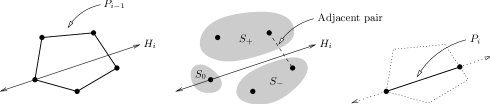
Figure 6: The inductive step of the double description method

The double description method is so named because at each stage it creates a “double description” of the working polytope $P_{i}$, both as the intersection $O\cap J\cap H_{1}\cap\ldots\cap H_{i}$ and as the convex hull of the vertex set $V_{i}$. The key inductive process of step 2 is depicted graphically in Figure 6.

There is one critical detail missing from this algorithm—we need some way of deciding whether two vertices $\mathbf{u},\mathbf{w}\in V_{i}$ are adjacent in the working polytope $P_{i}$. There are two primary methods, one algebraic and one combinatorial. Both methods are described by Fukuda and Prodon [12, Proposition 7]; we translate them here into the language of the projective solution space.

Definition 3.2 (Zero Set)

Consider any point $\mathbf{x}\in\mathbb{R}^{d}$. The zero set of $\mathbf{x}$, denoted $Z(\mathbf{x})$, is the set of indices at which $\mathbf{x}$ has zero coordinates. That is, $Z(\mathbf{x})=\{k\,|\,x_{k}=0\}$.

Zero sets are important because the non-negative orthant is bounded by the hyperplanes $x_{k}=0$. Thus $Z(\mathbf{x})$ indicates which facets of the non-negative orthant the point $\mathbf{x}$ belongs to.

Lemma 3.3 (Algebraic Adjacency)

Consider some polytope $P_{i}$ with vertices $\mathbf{u},\mathbf{w}$ in Algorithm 3.1. Then $\mathbf{u}$ and $\mathbf{w}$ are adjacent in $P_{i}$ if and only if the intersection of $H_{1}\cap\ldots\cap H_{i}$ with the hyperplanes $\{x_{k}=0\,|\,k\in Z(\mathbf{u})\cap Z(\mathbf{w})\}$ forms a subspace of dimension two.

Lemma 3.4 (Combinatorial Adjacency)

Consider some polytope $P_{i}$ with vertices $\mathbf{u},\mathbf{w}$ in Algorithm 3.1. Then $\mathbf{u}$ and $\mathbf{w}$ are adjacent in $P_{i}$ if and only if there is no other vertex $\mathbf{z}$ of $P_{i}$ for which $Z(\mathbf{z})\supseteq Z(\mathbf{u})\cap Z(\mathbf{w})$.

Neither condition is fast to test; the algebraic condition requires the rank of a matrix, and the combinatorial condition requires yet another loop through the vertices in $V_{i}$. The algebraic test is appealing, since it is not sensitive to the size of $V_{i}$ (which can grow very large). On the other hand, Fukuda and Prodon report better results with the combinatorial test, and argue that it should terminate early much of the time [12]. With regards to existing software, FXrays and Regina use the algebraic and combinatorial tests respectively.

We finish with a final implementation note. Although we define the problem in terms of vertices of the projective solution space, it is easier to work with extremal rays of the polyhedral cone $N=O\cap H_{1}\cap\ldots\cap H_{g}$, as defined in Definition 2.8. Abandoning the projective hyperplane allows us to use integer arithmetic instead of rational arithmetic, which is both faster and easier to implement. Both FXrays and Regina exploit this technique.

3.2 Filtering for Embedded Surfaces

One critical problem with polytope vertex enumeration is that the number of vertices can grow extremely large (this is quantified more precisely in Section 3.3). It is therefore in our interests to avoid generating “uninteresting” vertices if at all possible. The constraints of normal surface theory allow us to do just this, yielding spectacular improvements in running time.

Recall from Section 2 that we are only interested in vertices that represent embedded normal surfaces, and that every such vertex must satisfy the quadrilateral constraints (Definition 2.6). Each of these constraints identifies three coordinates $x_{i},x_{j},x_{k}$ (representing the three quadrilateral types in some tetrahedron), and insists that at most one of these coordinates is non-zero.

A naïve implementation might generate all vertices of the projective solution space and then discard those that do not satisfy the quadrilateral constraints. However, this does not make vertex enumeration any faster. Here we describe a filtering technique that discards such vertices at every intermediate stage of the double description method, thereby reducing the size of each set $V_{i}$ and speeding up the subsequent stages of the algorithm.

This filtering method is due to David Letscher, and was used in his proof-of-concept program Normal in 1999. It does not appear in the current literature, and so we describe it in detail here.

Definition 3.5 (Compatibility)

Two vectors $\mathbf{u},\mathbf{w}\in\mathbb{R}^{d}$ are said to be compatible if their sum $\mathbf{u}+\mathbf{w}$ satisfies the quadrilateral constraints.

It is useful to characterize compatibility and the quadrilateral constraints in terms of zero sets. The following results are both immediate consequences of Definitions 2.6 and 3.2:

Lemma 3.6

A vector $\mathbf{v}\in\mathbb{R}^{d}$ satisfies the quadrilateral constraints if and only if, for each tetrahedron of the underlying 3-manifold triangulation, $Z(\mathbf{v})$ is missing at most one quadrilateral coordinate for that tetrahedron.

Lemma 3.7

If vectors $\mathbf{u},\mathbf{w}\in\mathbb{R}^{d}$ contain only non-negative elements, then for any $\alpha,\beta>0$ we have $Z(\alpha\mathbf{u}+\beta\mathbf{w})=Z(\mathbf{u})\cap Z(\mathbf{w})$. In particular, $\mathbf{u}$ and $\mathbf{w}$ are compatible if and only if, for each tetrahedron of the underlying 3-manifold triangulation, $Z(\mathbf{u})\cap Z(\mathbf{w})$ is missing at most one quadrilateral coordinate for that tetrahedron.

It should be observed that all intermediate vertices obtained throughout the double description method are non-negative, since each intermediate polytope $P_{i}$ lies inside the non-negative orthant. Therefore Lemma 3.7 can be used in practice as a fast compatibility test. We return to this implementation detail in Section 4; in the meantime we proceed with the main filtering algorithm.

Algorithm 3.8 (Vertex Filtering)

Consider the double description method as outlined in Algorithm 3.1. Suppose we alter step 2(c), so that a pair $\mathbf{u}\in S_{+}$, $\mathbf{w}\in S_{-}$ is considered only if vectors $\mathbf{u}$ and $\mathbf{w}$ are compatible.

Then, in the resulting algorithm, each intermediate set $V_{i}$ will contain only those vertices of polytope $P_{i}$ that satisfy the quadrilateral constraints. In particular, the final set $V_{g}$ will contain only those vertices of the projective solution space $P=P_{g}$ that satisfy the quadrilateral constraints.

This algorithm is mostly easy to implement, though there is one important difficulty. Step 2(c) of the double description method requires us to determine whether two vectors are adjacent in the polytope $P_{i-1}$; however, since we have filtered out some vertices, we no longer have access to a complete description of $P_{i-1}$. Happily this turns out not to be a problem—we return to this adjacency issue after proving the main algorithm correct.

Proof.

Algorithm 3.8 is simple to prove by induction. To avoid confusion, let $V_{i}^{D}$ denote the vertex sets obtained using the original double description method, and let $V_{i}^{F}$ denote the new sets obtained using vertex filtering. Our claim is that $V_{i}^{F}$ contains precisely those vectors $\mathbf{v}\in V_{i}^{D}$ that satisfy the quadrilateral constraints.

To begin, we can observe that $V_{i}^{F}\subseteq V_{i}^{D}$ for each $i$, since filtering cannot create new vertices that were not there originally. It suffices therefore to consider the fate of each original vertex $\mathbf{v}\in V_{i}^{D}$. We proceed now with the main induction.

Our claim is certainly true for $V_{0}^{F}=V_{0}^{D}$, since these initial sets contain only unit vectors. Suppose the claim is true at stage $i-1$, and consider some original vertex $\mathbf{v}\in V_{i}^{D}$. There are two possible ways in which the original double description method could insert $\mathbf{v}$ into $V_{i}^{D}$:

1. Vector $\mathbf{v}$ is inserted during step 2(b). That is, $\mathbf{v}$ comes from the previous vertex set $V_{i-1}^{D}$ and is found to belong to the matching hyperplane $H_{i}$.

   Since vertex filtering does not affect step 2(b) of the double description method, the filtering algorithm inserts $\mathbf{v}$ into $V_{i}^{F}$ if and only if $\mathbf{v}$ is found in $V_{i-1}^{F}$. By our inductive hypothesis, this is true if and only if $\mathbf{v}$ satisfies the quadrilateral constraints.

2. Vector $\mathbf{v}$ is inserted during step 2(c). That is, $\mathbf{v}$ does not belong to the previous set $V_{i-1}^{D}$, but is instead created as the intersection $\overline{\mathbf{u}\mathbf{w}}\cap H_{i}$, where $\mathbf{u},\mathbf{w}\in V_{i-1}^{D}$ lie on opposite sides of the hyperplane $H_{i}$.

   We begin by noting that $\mathbf{v}=\alpha\mathbf{u}+\beta\mathbf{w}$ for some $\alpha,\beta>0$. There are two cases to consider:

   • If either $\mathbf{u}$ or $\mathbf{w}$ does not satisfy the quadrilateral constraints, then the combination $\mathbf{v}=\alpha\mathbf{u}+\beta\mathbf{w}$ cannot satisfy the quadrilateral constraints. By our inductive hypothesis, the pair $\mathbf{u},\mathbf{w}$ is not found in $V_{i-1}^{F}$ and so $\mathbf{v}$ is (correctly) not added to the new set $V_{i}^{F}$.

   • If both $\mathbf{u}$ and $\mathbf{w}$ satisfy the quadrilateral constraints then, by Lemmas 3.6 and 3.7, the new vertex $\mathbf{v}$ satisfies the quadrilateral constraints if and only if $\mathbf{u}$ and $\mathbf{w}$ are compatible. Here the filtering algorithm also acts correctly—the inductive hypothesis ensures that both $\mathbf{u},\mathbf{w}\in V_{i-1}^{F}$, and so the filtering algorithm adds $\mathbf{v}$ to $V_{i}^{F}$ if and only if $\mathbf{u}$ and $\mathbf{w}$ are compatible.

In each case we find that $\mathbf{v}$ is inserted into $V_{i}^{F}$ if and only if it satisfies the quadrilateral constraints, and so the induction is complete. ∎

We finish with a discussion of the different adjacency tests. The algebraic adjacency test (Lemma 3.3) does not rely on the vertex set $V_{i}$, and so we can use it unchanged with the filtering algorithm.

The combinatorial test (Lemma 3.4) is more of a problem, since it requires us to examine every vertex of the intermediate polytope $P_{i}$. This is impossible with the filtering method, where we deliberately throw away uninteresting vertices of $P_{i}$ to make the algorithm faster. Happily this does not matter, as seen in the following result.

Lemma 3.9 (Filtered Combinatorial Adjacency)

Consider some intermediate polytope $P_{i}$ in the vertex filtering algorithm, and let $V_{i}$ contain those vertices of $P_{i}$ that satisfy the quadrilateral constraints. If vertices $\mathbf{u},\mathbf{w}\in V_{i}$ are compatible, then they are adjacent in the polytope $P_{i}$ if and only if there is no other $\mathbf{z}\in V_{i}$ for which $Z(\mathbf{z})\supseteq Z(\mathbf{u})\cap Z(\mathbf{w})$.

Proof.

Suppose $\mathbf{u}$ and $\mathbf{w}$ are adjacent in $P_{i}$. By Lemma 3.4 there is no vertex $\mathbf{z}$ of $P_{i}$ for which $Z(\mathbf{z})\supseteq Z(\mathbf{u})\cap Z(\mathbf{w})$, and in particular there is no such $\mathbf{z}\in V_{i}$.

Alternatively, suppose $\mathbf{u}$ and $\mathbf{w}$ are not adjacent. By Lemma 3.4 there is some other vertex $\mathbf{z}$ of $P_{i}$ for which $Z(\mathbf{z})\supseteq Z(\mathbf{u})\cap Z(\mathbf{w})$. Because $\mathbf{u}$ and $\mathbf{w}$ are compatible, each tetrahedron has at most one quadrilateral coordinate missing from the set $Z(\mathbf{u})\cap Z(\mathbf{w})$ (Lemma 3.7). The same thing can therefore be said about the superset $Z(\mathbf{z})$, and so $\mathbf{z}$ satisfies the quadrilateral constraints (Lemma 3.6). Thus $\mathbf{z}\in V_{i}$, and the proof is complete. ∎

Vertex filtering is essential for any serious implementation of normal surface enumeration (and is used by all of the implementations discussed earlier). The only cost is the new compatibility test in step 2(c) of the double description method. On the other hand, vertex filtering can dramatically reduce the size of the vertex sets $V_{i}$, which cuts down both running time and memory usage as the double description method loops through these vertex sets.

As a final note, vertex filtering can also be applied to the sister problem of almost normal surface enumeration, where we introduce new “disc” types such as octagons and tubes. Embedded almost normal surfaces have additional rules, such as at most one quadrilateral or octagonal disc type per tetrahedron, and at most one octagon or tube in the entire surface. These rules yield new constraints of the form “at most one of the following coordinates may be non-zero”, whereupon similar filtering methods can be applied. The reader is referred to [20] for further discussion of almost normal surfaces.

3.3 Worst Cases and Pivoting Algorithms

Although the double description method is simple and elegant, it is unfortunately also very slow and very memory-hungry. We finish this overview with a discussion of just how bad things can get.

In many ways the double description method is not at fault—the difficulties are rooted in the problem it aims to solve. Dyer shows that counting the vertices of an arbitrary polytope is NP-hard [11], and Khachiyan et al. show that vertex enumeration over a polyhedron is NP-hard [24]; these results do not bode well.

At the very least, the running time is bounded below by the number of vertices (i.e., the size of the output), which for bounded polytopes can grow exponentially large in the polytope dimension. Specifically, for a polytope of dimension $p$ with $f$ facets, the upper bound theorem of McMullen [27] shows the worst case to be

number of vertices $$\leq {f-\lceil\frac{1}{2}p\rceil\choose\lfloor\frac{1}{2}p\rfloor}+{f-\lfloor\frac{1}{2}p\rfloor-1\choose\lceil\frac{1}{2}p\rceil-1}.$$

As an exercise, we can estimate this upper bound in the context of normal surface enumeration. Consider a one-vertex triangulation of a closed 3-manifold containing $n$ tetrahedra. Extending a result of Kang and Rubinstein [23], Tillmann [32] shows that the matching equations have a solution space of dimension $2n+1$. Taking the intersection with the projective hyperplane and the non-negative orthant in $\mathbb{R}^{d}$, it follows that the projective solution space is at worst a $2n$-dimensional polytope with $d$ facets. In the standard framework of Section 2 where $d=7n$, McMullen’s upper bound becomes $\frac{7}{6}{6n\choose n}$; in Tollefson’s quadrilateral space where $d=3n$ this bound becomes $\frac{3}{2}{2n\choose n}$. Using Stirling’s approximation, these bounds simplify to:

number of vertices in standard space $$\lesssim \frac{7}{2\sqrt{15\pi n}}\cdot\left(\frac{6^{6}}{5^{5}}\right)^{n}\ \simeq\ \frac{7}{2\sqrt{15\pi n}}\cdot 15^{n}$$

number of vertices in quadrilateral space $$\lesssim \frac{3}{2\sqrt{\pi n}}\cdot 4^{n}$$

Thus even in quadrilateral space, the number of vertices can potentially grow as $4^{n}$.

One critical weakness of the double description method is its memory consumption—since it involves looping through vertices of the intermediate polytopes $P_{i}$, its memory usage is linear in the number of such vertices (we return to this in detail in Section 4.4). Pivoting methods for polytope vertex enumeration are superior in this respect. In particular, Avis and Fukuda describe a pivoting algorithm that requires virtually no additional memory beyond storage of the input data [3]; this algorithm is further refined by Avis [1].

Although pivoting methods are appealing for the general vertex enumeration problem, they make it difficult to exploit the quadrilateral constraints. Pivoting methods essentially map out the vertices of a polytope by tracing out the simplex algorithm in reverse, moving from vertex to vertex using different styles of pivot. The difficulty is in finding a pivot that can “avoid” uninteresting vertices but still map out the remainder of the polytope. Indeed, there is no guarantee that the region of the polytope that satisfies the quadrilateral constraints is even connected, and in quadrilateral space it is easy to build examples where this is not the case.

Since even the fastest pivoting method remains bounded by the size of the output, it is essential that the quadrilateral constraints can be woven directly into the algorithm—one cannot afford to construct $4^{n}$ vertices in the worst case if the quadrilateral constraints are able to make this number orders of magnitude smaller. For this reason we focus on the double description method with vertex filtering, and leave pivoting methods for future work.

4 Optimizations

The algorithms of Section 3 describe a “vanilla” implementation of normal surface enumeration, as implemented for instance by older versions of the software package Regina. In this section we describe a series of optimizations that, as observed experimentally, yield substantial improvements in both running time and memory consumption. The relevant experiments and their results are summarized in Section 5.

The improvements presented here are offered as a guide for researchers seeking to code up their own implementations. Section 4.1 begins with a discussion of well-known but important implementation techniques, including bitmasks and cache optimization. Section 4.2 focuses on ordering the matching hyperplanes in a way that exploits the structure of the matching equations and quadrilateral constraints. In Section 4.3 we extend a technique of Fukuda and Prodon [12] that combines features of both the algebraic and combinatorial adjacency tests. Finally, Section 4.4 presents a technique in which we store and manipulate only “essential” properties of the intermediate vertices rather than the vertices themselves.

Memory consumption deserves a particular mention here. As noted in Section 3.3, both the running time and memory usage for the double description method are exponential in the worst case. Whilst running time is in theory an unbounded resource (as long as you are patient enough), memory is not—a typical personal computer has only a couple of gigabytes of fast memory. Once this is exhausted (which has happened to the author many times during normal surface enumeration), the computer borrows additional “virtual memory” from the hard drive. This virtual memory is much, much slower, and can have a severe impact not only on the performance of the algorithm but also on the entire operating system.

It is prudent therefore to give memory consumption just as high a priority as running time when working on the double description method. We address memory indirectly in Section 4.2, and focus on it explicitly with the techniques of Section 4.4.

4.1 Implementation Techniques

We begin our catalogue of optimizations with some simple implementation tricks. Though they are well-known, we include them here for reference because they have been found to improve the running time significantly.

• Bitmasks:
  Several components of the double description method work with zero sets of vectors. These include:

  • the combinatorial adjacency test (Lemmas 3.4 and 3.9), where we only consider a pair $\mathbf{u},\mathbf{w}\in V_{i}$ if there is no other $\mathbf{z}\in V_{i}$ for which $Z(\mathbf{z})\supseteq Z(\mathbf{u})\cap Z(\mathbf{w})$;

  • the compatibility test (Lemma 3.7), where we only consider a pair $\mathbf{u},\mathbf{w}\in V_{i}$ if the set $Z(\mathbf{u})\cap Z(\mathbf{w})$ is missing at most one quadrilateral coordinate for each tetrahedron.

  It is therefore convenient to store the zero set alongside each vector as we run through the double description algorithm. This can be done with almost no memory overhead using bitmasks. For instance, in dimension $d\leq 64$, an entire zero set $S$ can be stored using a single 64-bit integer (where the $i$th bit is set if and only if $i\in S$). For $d\leq 128$ this can be done using two 64-bit integers, and so on.

  Bitmasks are advantageous because they make set operations extremely fast—by using bitwise arithmetic on integers, the computer can effectively work on all elements of a set in parallel. For instance, if $d\leq 64$ then set intersection can be computing using the single C/C++ instruction ans = x & y, and subset relationships can be tested using the single C/C++ test if (x & y == y). Computing the size of a set (as required by the compatibility test) is a little more complex, but still fast; Warren [34] describes several clever methods that are far more efficient than looping through and testing each individual bit.

  Finally, bitmasks are not only cheap to store but also fast to construct. As the double description algorithm progresses, new vectors $\mathbf{v}\in V_{i}$ are created from old vectors $\mathbf{u},\mathbf{w}\in V_{i-1}$ by forming intersections of the form $\overline{\mathbf{u}\mathbf{w}}\cap H_{i}$. Lemma 3.7 shows that $Z(\mathbf{v})=Z(\mathbf{u})\cap Z(\mathbf{w})$, which can be computed using the fast set operations described above.

  It should be noted that the highly streamlined FXrays has used bitmasks for compatibility testing for many years (though it optimizes their application for some coordinate systems at the expense of others).

• Cache optimization:
  In his article on optimizing memory access [10], Drepper offers programmers advice on how to best utilize the CPU caches. One simple rule is that data that is accessed sequentially should be stored sequentially; this allows the CPU to prefetch large chunks of data from memory and work with the (much faster) caches instead. To illustrate, Drepper makes a naïve implementation of the matrix product $A\times B$ run over four times as fast simply by storing $A$ and $B$ in row major and column major order respectively—this works because the data storage follows the sequential order in which elements must be accessed to compute the term $(A\times B)_{i,j}=\sum_{k}A_{i,k}B_{k,j}$.

  In the double description method, where the vertex sets $V_{i}$ can grow extremely large, there is a temptation to use techniques that avoid large-scale allocations and deallocations of memory. For instance, we might partition vertices into the sets $S_{0}$, $S_{+}$ and $S_{-}$ in-place, without allocating additional temporary memory for these sets. However, because Algorithm 3.1 repeatedly iterates through these sets, Drepper’s article suggests that we should allocate new blocks of memory to store these sets sequentially as simple arrays (or, in C++, contiguous std::vector types). Likewise, we should avoid storing vertices in linked list structures—although vector data types require occasional large reallocations of memory, they maintain sequential data storage where linked lists do not.

  In theory the benefits of sequential data access should be well worth the cost of the extra memory allocation and deallocation, and the experimental evidence of Section 5 agrees.

4.2 Hyperplane Sorting

It is well known that the performance of the double description method is highly sensitive to the order in which the hyperplanes are processed. This is because the ordering of hyperplanes affects the size of each intermediate vertex set $V_{i}$, which in turn directly affects both running time and memory consumption—running time because step 2(c) of the double description method involves two nested loops over subsets $S_{+},S_{-}\subseteq V_{i-1}$, and memory consumption because the entire vertex set $V_{i}$ must be computed and stored at each stage, ready for use in the subsequent iteration of the main loop.

Avis et al. [2] present a series of heuristic options for this ordering, and proceed to manufacture cases in which each of them performs poorly; Fukuda and Prodon [12] also experiment with different heuristic orderings, and obtain best results with a lexicographic ordering (in which hyperplanes are sorted lexicographically according to their coefficient vectors). However, Avis et al. highlight the fact that no one heuristic is “universally good”, and that any additional knowledge about the problem at hand should be exploited if this is possible.

In the context of normal surface enumeration, we can exploit the following facts:

1. Each hyperplane comes from a single matching equation of the form $\mathbf{m}^{(i)}\cdot\mathbf{x}=0$. These matching equations are sparse—we can see from Definition 2.6 that each coefficient vector $\mathbf{m}^{(i)}$ has at most four non-zero coordinates.

2. The vertex filtering method strips out any vertices with “incompatible” non-zero quadrilateral coordinates. If we can use the matching equations to relate different quadrilateral coordinates within the same tetrahedron (in particular, force them to be non-zero), we can thereby hope that many vertices will be filtered out (thus keeping the vertex sets $V_{i}$ as small as possible).

We use observation (ii) to define a new ordering of hyperplanes. Essentially we start with matching equations that only involve the final few tetrahedra; gradually we incorporate more and more tetrahedra into our equations until the entire triangulation is covered. Since the matching equations are sparse, we expect this to be feasible. The result is as follows:

Algorithm 4.1 (Ordering of Matching Hyperplanes)

Consider some hyperplane $H$ in $\mathbb{R}^{d}$, defined by the matching equation $\mathbf{m}\cdot\mathbf{x}=0$. We define the position vector $\mathbf{p}(H)$ to be a $(0,1)$-vector of length $d$, where the $k$th element of $\mathbf{p}(H)$ is 0 or 1 according to whether the $k$th element of $\mathbf{m}$ is zero or non-zero respectively.

We now insert an extra step at the beginning of the double description method, which is to reorder the hyperplanes so that $\mathbf{p}(H_{1})\leq\mathbf{p}(H_{2})\leq\ldots\leq\mathbf{p}(H_{g})$. Here we treat $\leq$ as a lexicographic ordering of position vectors (so in dimension $d=3$ for instance, we have $(0,1,0)<(0,1,1)<(1,0,0)$ and so on).

Order Matching equation Coefficient vector $\mathbf{m}^{(i)}$ Position vector $\mathbf{p}(H_{i})$ 1 $q_{1,3}=q_{1,2}$ $0,\phantom{-}0,\phantom{-}0,\phantom{-}0,\phantom{-}0,-1,\phantom{-}1$ $0,~{}0,~{}0,~{}0,~{}0,~{}1,~{}1$ 2 $t_{1,2}+q_{1,2}=t_{1,4}+q_{1,1}$ $0,\phantom{-}1,\phantom{-}0,-1,-1,\phantom{-}1,\phantom{-}0$ $0,~{}1,~{}0,~{}1,~{}1,~{}1,~{}0$ 3 $t_{1,3}+q_{1,1}=t_{1,2}+q_{1,3}$ $0,-1,\phantom{-}1,\phantom{-}0,\phantom{-}1,\phantom{-}0,-1$ $0,~{}1,~{}1,~{}0,~{}1,~{}0,~{}1$ 4 $t_{1,3}+q_{1,3}=t_{1,2}+q_{1,1}$ $0,-1,\phantom{-}1,\phantom{-}0,-1,\phantom{-}0,\phantom{-}1$ $0,~{}1,~{}1,~{}0,~{}1,~{}0,~{}1$ 5 $t_{1,1}+q_{1,1}=t_{1,3}+q_{1,2}$ $1,\phantom{-}0,-1,\phantom{-}0,\phantom{-}1,-1,\phantom{-}0$ $1,~{}0,~{}1,~{}0,~{}1,~{}1,~{}0$

Table 1: Ordering the matching hyperplanes for the Gieseking manifold

This ordering is illustrated in Table 1 for the one-tetrahedron triangulation of the Gieseking manifold; it can be seen that the position vectors (though not the coefficient vectors) are indeed sorted lexicographically. The original matching equations are also included in the table, using the notation of Definition 2.6.

In general, the reason we use position vectors is so that equations involving only the final few tetrahedra will be processed relatively early, since their position vectors will begin with long strings of zeroes. Likewise, equations that involve the first coordinate of the first tetrahedron will be processed very late because their position vectors will begin with a one. We are therefore able to exploit observation (ii) as outlined above.

Like any other hyperplane ordering, Algorithm 4.1 is merely a heuristic. However, experimentation shows that it performs very well. This is seen in Section 5.3, where we compare it against several standard heuristics from the literature.

4.3 Filtering Pairs by Dimension

Recall from Section 3 that we have two options for testing whether vertices $\mathbf{u},\mathbf{w}\in V_{i}$ are adjacent in the intermediate polytope $P_{i}$. These are the algebraic adjacency test (Lemma 3.3), and the combinatorial adjacency test (Lemmas 3.4 and 3.9).

Fukuda and Prodon compare these tests experimentally, and find in their examples that the combinatorial test yields better results [12]. However, recall that the combinatorial test declares vertices $\mathbf{u},\mathbf{w}\in V_{i}$ adjacent if and only if there is no other $\mathbf{z}\in V_{i}$ for which $Z(\mathbf{z})\supseteq Z(\mathbf{u})\cap Z(\mathbf{w})$. This means that, in the worst case, the combinatorial test requires looping through the entire (possibly very large) vertex set $V_{i}$ in search for such a $\mathbf{z}$.

Fortunately we can break out of this loop early when $\mathbf{u}$ and $\mathbf{w}$ are non-adjacent (which is expected in the majority of cases)—we simply exit the loop when such a $\mathbf{z}$ is found. However, Fukuda and Prodon take this further and identify cases in which there is no need to loop at all. Their idea is to use properties of the algebraic test that only rely upon combinatorial data. Their result, translated into our formulation of the double description method, is as follows:

Lemma 4.2 (Dimensional Filtering)

Consider some intermediate polytope $P_{i}\subseteq\mathbb{R}^{d}$ in the double description method (Algorithm 3.1), formed as the intersection $P_{i}=O\cap J\cap H_{1}\cap H_{2}\cap\ldots\cap H_{i}$. If $\mathbf{u}$ and $\mathbf{w}$ are adjacent vertices of $P_{i}$, then

$$|Z(\mathbf{u})\cap Z(\mathbf{w})|+i\geq d-2.$$ (1)

This is an immediate consequence of the algebraic test (Lemma 3.3), which describes the intersection of $|Z(\mathbf{u})\cap Z(\mathbf{w})|+i$ hyperplanes as a subspace of dimension two. The real strength of Lemma 4.2 is that it only requires knowledge of the set $Z(\mathbf{u})\cap Z(\mathbf{w})$. Therefore we can use it as a fast prefilter for adjacency testing—for any pair of vertices $\mathbf{u},\mathbf{w}\in V_{i}$ we first check (1), and only run the full combinatorial test if the inequality holds.

We proceed now to strengthen the original result of Fukuda and Prodon. Our aim is to replace $i$ with a smaller number in the inequality (1), thus filtering out even more non-adjacent pairs $\mathbf{u},\mathbf{w}$. A trivial way to do this is to not count redundant hyperplanes—we can easily change the inequality to $|Z(\mathbf{u})\cap Z(\mathbf{w})|+\mathrm{rank}(i)\geq d-2$, where $\mathrm{rank}(i)$ is the number of independent hyperplanes in the collection $H_{1},\ldots,H_{i}$.

What is perhaps less obvious is that we can also avoid counting any hyperplane $H_{j}$ that does not slice between vertices of the previous set $V_{j-1}$ (even if this hyperplane is linearly independent of the others) and that this works even if $V_{j-1}$ is a filtered vertex set. The full result is as follows:

Lemma 4.3 (Extended Dimensional Filtering)

Consider the double description method (Algorithm 3.1), with or without vertex filtering (Algorithm 3.8). Let $H_{k}$ be some matching hyperplane, defined by the matching equation $\mathbf{m}^{(k)}\cdot\mathbf{x}=0$. We say that $H_{k}$ is pseudo-separating if there exist vertices $\mathbf{v}^{\prime},\mathbf{v}^{\prime\prime}\in V_{k-1}$ for which $\mathbf{m}^{(k)}\cdot\mathbf{v}^{\prime}<0<\mathbf{m}^{(k)}\cdot\mathbf{v}^{\prime\prime}$ (in other words, there are vertices of the old set $V_{k-1}$ on both sides of the hyperplane $H_{k}$). This definition is illustrated in Figure 7.

Now consider some intermediate polytope $P_{i}\subseteq\mathbb{R}^{d}$, with two compatible vertices $\mathbf{u},\mathbf{w}\in V_{i}$. If $\mathbf{u}$ and $\mathbf{w}$ are adjacent vertices of $P_{i}$, then

$$|Z(\mathbf{u})\cap Z(\mathbf{w})|+\mathrm{sep}(i)\geq d-2,$$ (2)

where $\mathrm{sep}(i)$ is the number of pseudo-separating hyperplanes in the list $H_{1},H_{2},\ldots,H_{i}$.

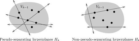
Figure 7: Illustrating pseudo-separating hyperplanes for a vertex set $V_{k-1}$

Before proving this result, we pause to make some observations. Not only is this result stronger than Lemma 4.2 (since it is clear that $\mathrm{sep}(i)\leq i$), but it is just as fast to test—we know when a hyperplane is pseudo-separating because the corresponding sets $S_{+}$ and $S_{-}$ are both non-empty in step 2(a) of the double description method.

It is again worth noting that Lemma 4.3 remains true even if we use vertex filtering. Because each filtered vertex set $V_{i}$ is potentially much smaller than the number of vertices of $P_{i}$, we can hope to see fewer pseudo-separating hyperplanes as a result (and thereby strengthen our dimensional filtering). Indeed, this behaviour is observed for many ideal triangulations in the cusped census of Callahan et al. [8].

We proceed with a proof of Lemma 4.3.

Proof.

The following argument assumes the double description method is used with vertex filtering. For the non-filtered case, simply remove all references to filtering in this proof.

Consider the polytope $P_{i}=O\cap J\cap H_{1}\cap\ldots\cap H_{i}$ as described in the statement of Lemma 4.3, and let $V_{i}$ be the filtered vertex set of $P_{i}$. In the list $H_{1},\ldots,H_{i}$, denote the pseudo-separating hyperplanes by $K_{1},\ldots,K_{p}$ and the non-pseudo-separating hyperplanes by $L_{1},\ldots,L_{q}$ (so that $p+q=i$). It is important that the hyperplanes in each new list be kept in the same order as in the original list $H_{1},\ldots,H_{i}$.

Define the new polytope $P_{i}^{\prime}$ to be the intersection $O\cap J\cap K_{1}\cap\ldots\cap K_{p}$ (i.e., the intersection of the unit simplex with only the pseudo-separating hyperplanes), and let $V_{i}^{\prime}$ be the filtered vertex set of $P_{i}^{\prime}$. Then the original polytope $P_{i}$ can be expressed as $P_{i}=P_{i}^{\prime}\cap L_{1}\cap\ldots\cap L_{q}$.

We can recover the original filtered vertices $V_{i}$ from $V_{i}^{\prime}$ using a “reordered” double description method. We begin with $P_{i}^{\prime}$ and its filtered vertices $V_{i}^{\prime}$, and then intersect each hyperplane $L_{1},\ldots,L_{q}$ in turn, as described by Algorithms 3.1 and 3.8.

In this reordered double description method, let $Q_{j}$ denote the intermediate polytope $Q_{j}=P_{i}^{\prime}\cap L_{1}\cap\ldots\cap L_{j}$, and let $W_{j}$ denote the filtered vertex set of $Q_{j}$ (in particular, $W_{0}=V_{i}^{\prime}$ and $W_{q}=V_{i}$). Then we can make the following observations:

1. Consider the stage of this new double description method where we intersect $Q_{j-1}$ with the hyperplane $L_{j}$ to form the polytope $Q_{j}$. Then one of the sets $S_{+}$ and $S_{-}$ as described in step 2(a) of Algorithm 3.1 is empty. That is, all of the vertices in the previous set $W_{j-1}$ lie on $L_{j}$ and/or to the same side of $L_{j}$.

   This can be seen as follows. Suppose $L_{j}$ appears as $H_{j^{\prime}}$ in the original list $H_{1},\ldots,H_{i}$. Then $Q_{j-1}=H_{1}\cap\ldots\cap H_{j^{\prime}-1}\cap K_{1}\cap\ldots\cap K_{p}$ (note that some hyperplanes might be repeated in this list). Therefore the filtered vertices of $Q_{j-1}$ are all convex combinations of the filtered vertices of $P_{j^{\prime}-1}=H_{1}\cap\ldots\cap H_{j^{\prime}-1}$, and since $H_{j^{\prime}}=L_{j}$ is not pseudo-separating, these vertices all lie on and/or to the same side of $L_{j}$.

2. From observation (i) above, the filtered vertex set $W_{j}$ of the intermediate polytope $Q_{j}$ is precisely $W_{j}=W_{j-1}\cap L_{j}$. That is, when we create $W_{j}$ in our reordered double description method, we simply keep those vertices of $W_{j-1}$ that lie in the hyperplane $L_{j}$ and throw the others away. In particular, because one of $S_{+}$ and $S_{-}$ is empty, no new vertices can be created.

3. Following observation (ii) to its conclusion, the vertex sets satisfy

   $$V_{i}^{\prime}=W_{0}\supseteq W_{1}\supseteq\ldots\supseteq W_{q}=V_{i}.$$

   As a side note, although $V_{i}^{\prime}\supseteq V_{i}$, it is not necessarily true that all unfiltered vertices of $P_{i}$ are also vertices of $P_{i}^{\prime}$. This is because pseudo-separation is defined only in terms of filtered vertices.

Now consider two compatible vertices $\mathbf{u},\mathbf{w}\in V_{i}$. Observation (iii) shows that $\mathbf{u}$ and $\mathbf{w}$ are vertices of each polytope $Q_{j}$. Let $F_{j}$ be the (unique) minimal-dimensional face of $Q_{j}$ containing both $\mathbf{u}$ and $\mathbf{w}$. We can make the following observations about each face $F_{j}$:

1. Every vertex of $F_{j}$ is in the filtered set $W_{j}$.

   This can be shown using zero sets. Let $X\subseteq\mathbb{R}^{d}$ be the subspace formed by setting every coordinate in $Z(\mathbf{u})\cap Z(\mathbf{w})$ equal to zero. That is,

   $$X=\{\mathbf{x}\,|\,x_{i}=0\ \mbox{for all}\ i\in Z(\mathbf{u})\cap Z(\mathbf{w})\}.$$

   Because $Q_{j}$ is a polytope in the non-negative orthant, each equation $x_{i}=0$ is a supporting hyperplane for $Q_{j}$. Therefore $X\cap Q_{j}$ is a face of $Q_{j}$, and moreover contains both $\mathbf{u}$ and $\mathbf{w}$. By minimality, $F_{j}$ is a subface of $X\cap Q_{j}$, and so every vertex of $F_{j}$ lies in $X$.

   Because $\mathbf{u}$ and $\mathbf{w}$ are compatible, Lemma 3.7 shows that $Z(\mathbf{u})\cap Z(\mathbf{w})$ is missing at most one quadrilateral coordinate per tetrahedron. This means that every point in $X$ satisfies the quadrilateral constraints, and in particular, so do the vertices of $F_{j}$. Thus the vertices of $F_{j}$ (which are also vertices of the enclosing polytope $Q_{j}$) belong to the filtered set $W_{j}$.

2. For each $j$, the faces $F_{j-1}$ and $F_{j}$ are identical.

   This follows from our earlier observations. From (iv) and (i) we see that $L_{j}$ is a supporting hyperplane for $F_{j-1}$, and so $F_{j-1}\cap L_{j}$ is a subface of $F_{j-1}$ containing $\mathbf{u}$ and $\mathbf{w}$; by minimality it follows that $F_{j-1}\cap L_{j}=F_{j-1}$.

   On the other hand, since $F_{j-1}$ is a face of the polytope $Q_{j-1}$, we see that $F_{j-1}\cap L_{j}$ is a face of $Q_{j-1}\cap L_{j}=Q_{j}$, again containing both $\mathbf{u}$ and $\mathbf{w}$. Thus $F_{j}$ is a subface of $F_{j-1}\cap L_{j}=F_{j-1}$, and by minimality again it follows that $F_{j}=F_{j-1}$.

3. Carrying observation (v) to its conclusion, we have $F_{0}=F_{1}=\ldots=F_{q}$.

We are finally ready to examine the problem of adjacency. Vertices $\mathbf{u}$ and $\mathbf{w}$ are adjacent in the polytope $Q_{j}$ if and only if the face $F_{j}$ is an edge. From observation (vi) it follows that $\mathbf{u}$ and $\mathbf{w}$ are adjacent in $P_{i}^{\prime}=Q_{0}$ if and only if they are adjacent in $P_{i}=Q_{q}$.

Our main result (Lemma 4.3) now follows immediately by applying the earlier Lemma 4.2 to the polytope $P_{i}^{\prime}$. ∎

We conclude with a note regarding further generalizations of Lemma 4.3. A key property of non-pseudo-separating hyperplanes is that, in the double description method, they do not create any new vertices (though they can remove old ones).

We might hope therefore to extend Lemma 4.3 to “avoid counting” all hyperplanes with this property; for instance, we might hope to avoid hyperplanes that are pseudo-separating but that do not produce any compatible pairs of vertices on either side. It turns out that this cannot be done—although counterexamples are extremely rare, they can be found.

4.4 Inner Product Representation

Recall from the opening notes of Section 4 that memory (unlike time) is often a resource with hard limits, and that the worst cases for the double description method are exponential in memory as well as time. In our final improvement to the double description method, we take aim directly at memory consumption.

The high memory usage of the double description method comes almost entirely from storing the intermediate vertex sets $V_{i}$. Traditionally each vertex is stored as a sequence of coordinates in $\mathbb{R}^{d}$, though in Section 4.1 we extend this marginally by adding a bitmask for the zero set. Therefore, if we are to reduce memory usage, we have one of two options:

• Find a way to reduce the sizes of the vertex sets $V_{i}$, which is the approach taken in Section 4.2;

• Find a way to avoid storing the full coordinates of each vertex, which is the approach that we take here.

Our strategy therefore is to discard the individual coordinates of each vertex $\mathbf{v}\in V_{i}$, and instead to store only “essential information” from which we can recover the full coordinates if we need to. In fact we already have this essential information—it is all contained in the zero set $Z(\mathbf{v})$.

Lemma 4.4

At any stage of the double description method, the zero set $Z(\mathbf{v})$ contains sufficient information to recover the entire vertex $\mathbf{v}\in V_{i}$. More precisely, the full coordinates of $\mathbf{v}$ can be recovered by solving the following simultaneous equations:

• the matching equations $\mathbf{m}^{(k)}\cdot\mathbf{v}=0$ for $k=1,\ldots,i$;

• the projective equation $\sum v_{j}=1$;

• the facet equations $v_{j}=0$ for each $j\in Z(\mathbf{v})$.

Proof.

This is an immediate consequence of the fact that a vertex of a polytope is the intersection of the facets that it belongs to. For each intermediate polytope $P_{i}$, the facets of $P_{i}$ are described by inequalities of the form $x_{j}\geq 0$ (deriving from the non-negative orthant). The facets that a vertex $\mathbf{v}$ belongs to are those for which $v_{j}=0$, that is, those corresponding to coordinate positions $j\in Z(\mathbf{v})$. ∎

What Lemma 4.4 shows is that we could store only the zero sets of our vertices, with no coordinates whatsoever. Because zero sets are stored as bitmasks that take very little space (Section 4.1), this would be a magnificent improvement in memory consumption. However, it could slow down our algorithm terribly, since we would need to solve the equations of Lemma 4.4 each time we wanted to analyze or manipulate any vertex $\mathbf{v}\in V_{i}$.

If we analyze the algorithms and improvements of Sections 3 and 4, we find that the only operations we need to perform on vertices are the following:

1. Creating $d$ unit vectors for the initial set $V_{0}$;

2. Testing the sign of $\mathbf{m}^{(i)}\cdot\mathbf{v}$ for $\mathbf{v}\in V_{i-1}$;

3. Creating a new vertex $\mathbf{v}=\overline{\mathbf{u}\mathbf{w}}\cap H_{i}$ from two old vertices $\mathbf{u},\mathbf{w}\in V_{i-1}$, which is done by computing

   $$\mathbf{v}=\frac{(\mathbf{m}^{(i)}\cdot\mathbf{u})\mathbf{w}-(\mathbf{m}^{(i)}\cdot\mathbf{w})\mathbf{u}}{(\mathbf{m}^{(i)}\cdot\mathbf{u})-(\mathbf{m}^{(i)}\cdot\mathbf{w})}\ ;$$

4. Manipulations involving zero sets (such as compatibility testing, the combinatorial adjacency test, or extended dimensional filtering);

5. Outputting the final solutions, as stored in the final vertex set $V_{g}$.

The only non-trivial operation in this list is the inner product $\mathbf{m}^{(i)}\cdot\mathbf{v}$, which suggests storing vectors using the following representation:

Definition 4.5 (Inner Product Representation)

Consider some vertex $\mathbf{v}\in V_{i}$ in the double description method (Algorithm 3.1). We define the inner product representation $I(\mathbf{v})$ to be the $(g-i)$-dimensional vector

$$\left(\mathbf{m}^{(i+1)}\cdot\mathbf{v},~{}\mathbf{m}^{(i+2)}\cdot\mathbf{v},~{}\ldots,~{}\mathbf{m}^{(g)}\cdot\mathbf{v}\right),$$

recalling that there are $g$ matching equations in total.

We use the inner product representation by storing $I(\mathbf{v})$ instead of the full coordinates for each intermediate vertex $\mathbf{v}\in V_{i}$. We continue to store the zero sets $Z(\mathbf{v})$ as bitmasks so that (by Lemma 4.4) no information is lost.

In general, the inner product representation is cheaper to store than the full coordinates of a vertex, and grows significantly cheaper still as the algorithm progresses. In the standard coordinate system of Section 2, we work in dimension $d=7n$ but have at most $g\leq 6n$ matching equations. In Tollefson’s quadrilateral coordinates we work in dimension $d=3n$ but (assuming a closed one-vertex triangulation) have a mere $n+1$ matching equations. As a result, our algorithm starts out using a modest $6/7$ or $1/3$ of the original storage respectively, and as $i\to g$ in the later stages of the algorithm our memory consumption shrinks almost to zero. By the time we reach $i=g$ the only storage remaining is the (very cheap) bitmasks for our zero sets.

It is important that the greatest benefits of the inner product representation arise in the later stages of the algorithm. Anecdotal evidence (observed time and time again) suggests that the worst explosions of vertex sets $V_{i}$ tend to occur in later stages of the algorithm. This means that our new representation focuses its optimizations where they are needed the most.

While the inner product representation gives a significant improvement in memory consumption, it is important to understand how it affects running time. We therefore consider each of the five vertex operations listed earlier:

1. Creating $d$ unit vectors for the initial set $V_{0}$ is easy. If $\mathbf{v}_{j}$ is the $j$th unit vector, then the elements of $I(\mathbf{v}_{j})$ are the $j$th coordinates of the matching equations $\mathbf{m}^{(1)},\ldots,\mathbf{m}^{(g)}$.

2. Testing the sign of $\mathbf{m}^{(i)}\cdot\mathbf{v}$ for $\mathbf{v}\in V_{i-1}$ is very easy; we simply look at the first element of $I(\mathbf{v})$.

3. Computing the intersection $\mathbf{v}=\overline{\mathbf{u}\mathbf{w}}\cap H_{i}$ for $\mathbf{u},\mathbf{w}\in V_{i-1}$ and $\mathbf{v}\in V_{i}$ is much the same as in the standard algorithm. Using

   $$\mathbf{v}=\frac{(\mathbf{m}^{(i)}\cdot\mathbf{u})\mathbf{w}-(\mathbf{m}^{(i)}\cdot\mathbf{w})\mathbf{u}}{(\mathbf{m}^{(i)}\cdot\mathbf{u})-(\mathbf{m}^{(i)}\cdot\mathbf{w})}$$

   it is easy to show that

   $$I(\mathbf{v})=\mathrm{trunc}\left[\frac{\mathrm{head}[I(\mathbf{u})]\,I(\mathbf{w})-\mathrm{head}[I(\mathbf{w})]\,I(\mathbf{u})}{\mathrm{head}[I(\mathbf{u})]-\mathrm{head}[I(\mathbf{w})]}\right],$$

   where $\mathrm{head}[\ldots]$ denotes the first element of a vector, and where $\mathrm{trunc}[\ldots]$ indicates removing the first element from a vector.

4. Manipulations involving zero sets are all done using bitmasks, and are not affected at all by the change in vector representation.

5. Outputting the final solutions requires us to solve the equations of Lemma 4.4 for each vertex in the final set $V_{g}$.

The running times for these operations under both old and new vertex representations are listed in Table 2 (excluding zero set manipulations, which are irrelevant here). Since $g<d$ in general, we find that most of these operations are in fact faster using the inner product representation.

Operation Full coordinate rep. Inner product rep. Creating $d$ unit vectors $O(d^{2})$ $O(gd)$ Testing sign of $\mathbf{m}^{(i)}\cdot\mathbf{v}$ $O(d)$ $O(1)$ Computing $\overline{\mathbf{u}\mathbf{w}}\cap H_{i}$ $O(d)$ $O(g)$ Outputting final solutions $O(|V_{g}|)$ $O(g^{2}d\cdot|V_{g}|)$

Table 2: Time complexities for various vertex operations

There is only one operation for which the inner product representation is slower, which is outputting the final solutions. Here we must solve a full system of equations for each vertex in $V_{g}$ (the complexity estimate in Table 2 assumes a simple implementation using matrix row operations). However:

• The output operation does not happen often. We only output solutions at the very end of the algorithm, unlike operations such as $\mathbf{m}^{(i)}\cdot\mathbf{v}$ or $\overline{\mathbf{u}\mathbf{w}}\cap H_{i}$ which we perform many times at every stage of the double description method.

• The number of systems of equations we must solve is $|V_{g}|$, which is not large. Experimental evidence suggests that the final solution set $V_{g}$ is typically small, often orders of magnitude smaller than the worst intermediate vertex sets $V_{i}$ (see for instance Table 3 in the following section). This is likely due to the quadrilateral constraints—as we enforce more matching equations, we are forced to make more quadrilateral coordinates non-zero, and we can filter out more vertices as a result.

We hope therefore that this extra cost in outputting the final solutions is insignificant, and indeed this is seen experimentally in Section 5.1—the losses in the output operation are far outweighed by the other gains described above, and the inner product representation yields better performance in both memory usage and running time.

5 Experimentation

Having developed several improvements to the normal surface enumeration algorithm, we now road-test these improvements using a collection of real examples, measuring both running time and memory consumption.

In the following tests, we enumerate surfaces in both the standard coordinate system of Section 2 and the quadrilateral coordinates of Tollefson [33]. We include both systems because they have some interesting differences:

• The matching equations in standard coordinates are all sparse, whereas in quadrilateral coordinates they are only sparse on average (in particular, dense equations are infrequent but possible).

• The quadrilateral constraints (and hence vertex filtering) involve all coordinate positions in quadrilateral coordinates, but only $3/7$ of the coordinate positions in standard coordinates.

• Quadrilateral coordinates work in a smaller dimension than standard coordinates ($3n<7n$), allowing us to run tests on larger and more interesting triangulations.

For further information on quadrilateral coordinates and the corresponding matching equations, the reader is again referred to [33].

We use 19 different triangulations for our tests: eleven closed hyperbolic triangulations are used as “ordinary” cases, and eight twisted layered loops are used for extreme “stress testing”. In detail:

• The closed hyperbolic triangulations are drawn arbitrarily from the Hodgson-Weeks census of small-volume closed hyperbolic 3-manifolds [17]. These include six smaller cases ($9\leq n\leq 13$) for use with standard coordinates, and five larger cases ($16\leq n\leq 20$) for use with quadrilateral coordinates.

• An $n$-tetrahedron twisted layered loop is an extremely well structured triangulation of the quotient space $S^{3}/Q_{4n}$. Twisted layered loops are conjectured by Matveev to have minimal complexity [26], and a proof of this claim has recently been announced by Jaco, Rubinstein and Tillmann [21]. Here we include four smaller cases ($9\leq n\leq 18$) for standard coordinates, and four larger cases ($30\leq n\leq 75$) for quadrilateral coordinates.

  The following properties make twisted layered loops ideal for stress testing:

  • The tight structure of these triangulations makes vertex filtering extremely powerful, allowing us to run tests on very large triangulations (up to 75 tetrahedra for quadrilateral coordinates).

  • In standard coordinates, the final solution set $V_{g}$ contains an exponential number of vertices (specifically $F_{n-1}+2F_{n-2}+1$, where $F_{0}=1$, $F_{1}=1$, …are the Fibonacci numbers). Moreover, this is observed to be much larger than the final solution set for most census triangulations of similar size.

  • In contrast, in quadrilateral coordinates the final solution set contains a linear number of vertices (specifically $n+1$), which is observed to be very small amongst census triangulations of similar size.

  The reader is referred to [7] for details on the final two points, and in particular for proofs of the formulae $|V_{g}|=F_{n-1}+2F_{n-2}+1$ and $|V_{g}|=n+1$.

Tetrahedra Hyp. volume Final set $|V_{g}|$ Max of any $|V_{i}|$ Dimension $d$ Standard coordinates 9(b) 0.94270736 19 899 63 10(b) 1.75712603 30 873 70 11(b) 2.10863613 45 2 221 77 12(a)(b) 2.93565190 64 3 477 84 12(b) 3.02631753 54 941 84 13(b) 3.08076667 59 1 891 91 Quadrilateral coordinates 16(b) 4.27796055 48 6 655 48 17(b) 4.30972819 33 4 025 51 18(b) 4.40945629 68 3 335 54 19(b) 4.58232390 95 15 988 57 20(b) 4.68714601 156 47 317 60

Table 3: Statistics for the “ordinary” closed hyperbolic triangulations

Tetrahedra Quotient space Final set $|V_{g}|$ Max of any $|V_{i}|$ Dimension $d$ Standard coordinates 9 $S^{3}/Q_{36}$ 77 375 63 12 $S^{3}/Q_{48}$ 323 1 585 84 15 $S^{3}/Q_{60}$ 1 365 6 711 105 18 $S^{3}/Q_{72}$ 5 779 28 425 126 Quadrilateral coordinates 30 $S^{3}/Q_{120}$ 31 171 90 45 $S^{3}/Q_{180}$ 46 261 135 60 $S^{3}/Q_{240}$ 61 351 180 75 $S^{3}/Q_{300}$ 76 441 225

Table 4: Statistics for the “extreme case” twisted layered loops

Tables 3 and 4 give an overview of the 19 triangulations chosen for testing; the two tables cover the hyperbolic triangulations and the twisted layered loops respectively. The columns in each table include:

1. The number of tetrahedra $n$. The hyperbolic set includes two 12-tetrahedron triangulations; these are labelled 12(a) and 12(b) for later reference.

2. The hyperbolic volume in Table 3, and the quotient space in Table 4. This information, combined with the tables from the Hodgson-Weeks census [17], uniquely identifies each 3-manifold.

3. The size of the final solution set $V_{g}$.

4. The maximum size of any intermediate vertex set $V_{i}$, under an algorithm that uses all of the improvements of Section 4.

5. The dimension of the underlying vertex enumeration problem, which is $7n$ or $3n$ for standard or quadrilateral coordinates respectively.

The maximum $|V_{i}|$ figures are particularly interesting. In Table 3 they highlight the observation that, for “ordinary” triangulations, the intermediate sets $V_{i}$ can grow orders of magnitude larger than the final set $V_{g}$. In Table 4 they highlight the strength of vertex filtering in the highly structured twisted layered loops, where the vertex sets $V_{i}$ are kept small from start to finish.

The remainder of this section is structured as follows. In Section 5.1 we consider the various improvements presented in this paper and examine their effect on running time for each of our 19 triangulations. Likewise, Section 5.2 offers a similar analysis of memory consumption. In Section 5.3 we evaluate our heuristic ordering of hyperplanes in more detail, comparing it against other standard orderings from the literature. All experiments are conducted on a 2.4 GHz Intel Core 2 machine using the software package Regina [4, 5].

5.1 Improvements in Running Time

We begin our series of experiments with an analysis of running time. Our aim here is to measure the strength of each individual improvement presented in Section 4.

As a starting point, we begin with the standard double description method with vertex filtering, as described in Algorithms 3.1 and 3.8. We then refine the algorithm, adding one improvement at a time, until we arrive at a final algorithm that incorporates all of the optimizations described in this paper.

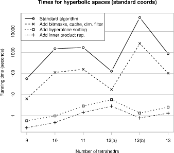
Figure 8: Improvements in running time for major optimizations

A summary of results is presented in Figure 8, which compares the following variants:

1. The standard algorithm, as outlined above.

2. The standard algorithm with bitmasks and cache optimization (Section 4.1) and dimensional filtering (Section 4.3). Because each of these optimizations yields only a minor improvement on its own, they are bundled together to simplify the graphs.

3. All of the previous improvements plus hyperplane sorting (Section 4.2).

4. All of the previous improvements plus the inner product representation (Section 4.4).

It should be noted that Figure 8 is plotted on a log scale, which means that each horizontal bar represents a factor of ten improvement. Given this, the results are extremely pleasing—the final algorithm (iv) is often 100 or 1 000 faster than the original (i), and for one case it runs over 50 000 times faster.

The weakest improvement is seen with the twisted layered loops using standard coordinates, where the size of the final solution set is known to be exponential; here the bitmasks and cache optimization provide most of the gains. Nevertheless, even in these extreme scenarios, both hyperplane sorting and the inner product representation independently double the speed for the large case $n=18$, and the final algorithm is still $\simeq 50$ times as fast as the original.

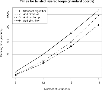
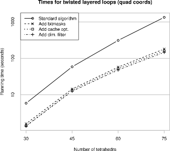
Figure 9: Details for bitmasks, cache optimization and dimensional filtering

Because bitmasks, cache optimization and dimensional filtering are bundled together in the main summary of results, we separate them out in Figure 9 to show their individual effects. Once more we see the extreme nature of the twisted layered loops—although all three improvements are effective on the hyperbolic spaces, some improvements (particularly dimensional filtering) have very little effect on the twisted layered loops.

It is worth noting that in the best cases, such as where the final algorithm is $>1\,000$ times or even $>10\,000$ times faster, the bulk of the gains are due to hyperplane sorting. We return to hyperplane sorting in greater detail in Section 5.3.

5.2 Improvements in Memory Usage

We continue our series of experiments by measuring the memory consumption of different variants of our algorithm. The results are plotted in Figure 10, where again we bundle together bitmasks, cache optimization and dimensional filtering for simplicity.

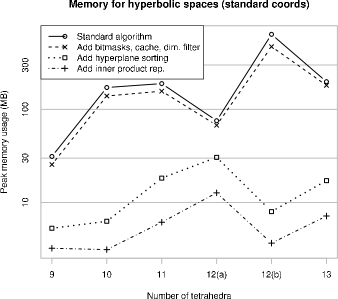
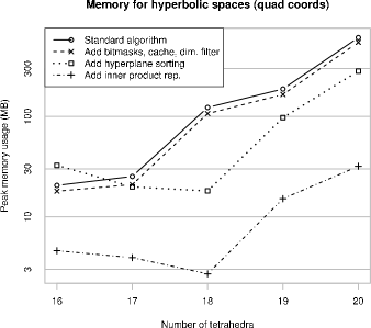
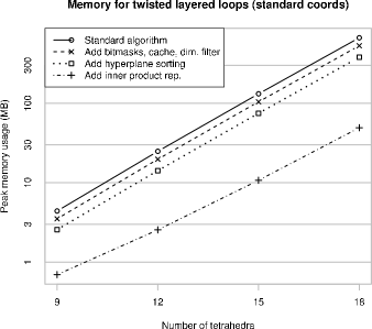
Figure 10: Improvements in memory usage for major optimizations

To be precise, Figure 10 measures peak memory usage, which is defined to be the maximum memory usage at any stage of the algorithm minus the memory usage at the beginning of the algorithm. This means that we only count memory that is genuinely used by the vertex enumeration algorithm, and not unrelated overhead such as system libraries or the storage of the program itself. We measure memory in megabytes, which we take to mean $10^{6}$ bytes (not $2^{20}$ bytes which is sometimes used instead).

Once more, the results are plotted on a log scale; here every two horizontal bars represent a factor of ten improvement (with a single bar representing approximately a factor of three). Again the results are extremely pleasing—for the large cases we are able to reduce memory consumption by factors of around 15 to 85, and in one hyperbolic case by a factor of 175.

It is particularly interesting to examine memory consumption for the twisted layered loops. These cases are extreme in both senses—in standard coordinates we see our weakest improvements (a factor of $14$ for $n=18$), and in quadrilateral coordinates we see some of our strongest improvements (a factor of $84$ for $n=75$). This is not entirely surprising, since we know that twisted layered loops have extremely large and extremely small solution sets in standard and quadrilateral coordinates respectively.

5.3 Comparison of Hyperplane Orderings

It is noted by Fukuda and Prodon [12] that the ordering of hyperplanes is critically important for a fast implementation of the double description method. This matches our experimental observations—whereas most optimizations are consistent in the way they reduce running time and memory consumption, hyperplane ordering is much more variable. Sometimes we only achieve mild improvements through ordering the hyperplanes, and other times we achieve spectacular results.

The reason that hyperplane ordering has such power is because, unlike any of our other optimizations, it affects the sizes of the intermediate vertex sets $V_{i}$. By keeping these sets small and taming the exponential explosion, we can achieve magnificent improvements in both running time and memory usage; on the other hand, if we inadvertently encourage the exponential explosion then the results can be disastrous.

It is therefore prudent to compare our ordering by position vectors (Algorithm 4.1) against other standard orderings from the literature. The other orderings we consider are:

• No ordering:
  We do not order the hyperplanes at all, but merely process them in the order in which they are constructed. Note that this is not a “random” ordering; in the case of Regina, the hyperplanes are constructed in an order that (in a rough sense) moves the non-zero coefficients from the first tetrahedron to the last. This is because each matching equation involves a face of the triangulation, and Regina happens to number faces internally in a similar manner.

• Dynamic ordering:
  Here we reorder the hyperplanes on the fly. Recall from Algorithm 3.1 that each hyperplane $H_{i}$ is used to divide the vertices of $V_{i-1}$ into sets $S_{0}$, $S_{+}$ and $S_{-}$, whereupon we embark upon the slow task of examining all pairs $\mathbf{u}\in S_{+}$ and $\mathbf{v}\in S_{-}$. With a dynamic ordering, we choose the hyperplane $H_{i}$ so that the number of pairs $|S_{+}|\times|S_{-}|$ is as small as possible.

  This is essentially the dynamic mixcutoff ordering defined by Avis et al. [2], adapted to make better use of the set $S_{0}$ (whose vertices do not need processing). Other dynamic orderings appear in the literature, notably mincutoff and maxcutoff [2, 12], but these are defined for intersections of half-spaces and are less relevant for intersections of hyperplanes.

• Lexicographic ordering:
  With lexicographic ordering we simply sort the hyperplanes by their coefficient vectors, possibly after performing some normalization. Fukuda and Prodon report good results using this method [12].

  Lexicographic orderings are typically defined for intersections of half-spaces, where the sign of each vector is well-defined. Since we are dealing with intersections of hyperplanes, sign does not matter (so the coefficient vector $-\mathbf{m}$ is just as good as $\mathbf{m}$).

  We consider two ways of choosing the sign of each vector:

  • Positive first, where we ensure that the first non-zero entry in each coefficient vector is positive;

  • Random signs, where the sign of each vector is selected at random.

Figure 11: Running times for various hyperplane orderings (set 1/2)

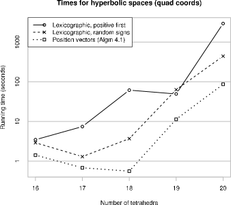
Figure 12: Running times for various hyperplane orderings (set 2/2)

The running times for various lexicographic orderings are presented in Figures 11 and 12. Figure 11 compares our Algorithm 4.1 against no ordering and dynamic ordering, and Figure 12 compares Algorithm 4.1 against both variants of the lexicographic ordering. Both figures again use a log scale (with each horizontal bar representing a factor of ten), and the algorithms incorporate all of our other improvements (bitmasks, cache optimization, dimensional filtering and inner product representation).

It is pleasing to see that our Algorithm 4.1 performs better than the others in most cases, and is the only ordering that performs consistently well. The only serious competitor is the dynamic ordering, which performs a little better in some cases; however, for some of the hyperbolic spaces the dynamic ordering runs $10\,000$ times slower.

As a final note, Figure 12 is missing a data point. This is because the random first lexicographic ordering for the $n=18$ twisted layered loop was stopped manually after two days; extrapolation suggests that it could have run for weeks before finishing.

6 Conclusion

In this paper we outline the standard algorithm for enumerating normal surfaces in a 3-manifold triangulation, by combining the double description method of Motzkin et al. with the vertex filtering method of Letscher. Following this we describe four optimizations:

• Bitmasks and cache optimization, which are well-known implementation techniques that can be applied to the double description method;

• Hyperplane sorting, where we order the matching hyperplanes according to their position vectors;

• Dimensional filtering, where we extend a result of Fukuda and Prodon to avoid processing certain pairs of vertices;

• The inner product representation, where we store only essential properties of the vertices instead of the full vertex coordinates.

We find that all of these techniques are successful in reducing running time, with dimensional filtering the weakest (though still effective in most cases) and hyperplane sorting the strongest (sometimes cutting running time by several orders of magnitude). The optimizations that focus on memory are also successful in reducing memory consumption by significant factors (though not as large as running time). Furthermore, the hyperplane ordering that we define here performs consistently well against other orderings from the literature.

Whilst these results are extremely promising, readers are encouraged to try these techniques for themselves—as other authors have noted, the performance of the double description method is highly variable, and different examples can reward or penalize different optimizations [2, 12]. Nevertheless, the techniques presented here are found to perform consistently well, and are offered as a basis for further optimizations.

Benjamin A. Burton
Department of Mathematics, SMGS, RMIT University
GPO Box 2476V, Melbourne, VIC 3001, Australia
(bab@debian.org)

References

- [1] David Avis, A revised implementation of the reverse search vertex enumeration algorithm, Polytopes—Combinatorics and Computation (Oberwolfach, 1997), DMV Sem., vol. 29, Birkhäuser, Basel, 2000, pp. 177–198.
- [2] David Avis, David Bremner, and Raimund Seidel, How good are convex hull algorithms?, Comput. Geom. 7 (1997), no. 5-6, 265–301.
- [3] David Avis and Komei Fukuda, A pivoting algorithm for convex hulls and vertex enumeration of arrangements and polyhedra, Discrete Comput. Geom. 8 (1992), no. 3, 295–313.
- [4] Benjamin A. Burton, Regina: Normal surface and 3-manifold topology software, http://regina.sourceforge.net/, 1999–2009.
- [5] , Introducing Regina, the 3-manifold topology software, Experiment. Math. 13 (2004), no. 3, 267–272.
- [6] , Enumeration of non-orientable 3-manifolds using face-pairing graphs and union-find, Discrete Comput. Geom. 38 (2007), no. 3, 527–571.
- [7] , Extreme cases in normal surface enumeration, In preparation, 2009.
- [8] Patrick J. Callahan, Martin V. Hildebrand, and Jeffrey R. Weeks, A census of cusped hyperbolic 3-manifolds, Math. Comp. 68 (1999), no. 225, 321–332.
- [9] Marc Culler and Nathan Dunfield, FXrays: Extremal ray enumeration software, http://www.math.uic.edu/~t3m/, 2002–2003.
- [10] Ulrich Drepper, What every programmer should know about memory, http://people.redhat.com/drepper/cpumemory.pdf, November 2007.
- [11] M. E. Dyer, The complexity of vertex enumeration methods, Math. Oper. Res. 8 (1983), no. 3, 381–402.
- [12] Komei Fukuda and Alain Prodon, Double description method revisited, Combinatorics and Computer Science (Brest, 1995), Lecture Notes in Comput. Sci., vol. 1120, Springer, Berlin, 1996, pp. 91–111.
- [13] Wolfgang Haken, Theorie der Normalflächen, Acta Math. 105 (1961), 245–375.
- [14] , Über das Homöomorphieproblem der 3-Mannigfaltigkeiten. I, Math. Z. 80 (1962), 89–120.
- [15] Joel Hass, Jeffrey C. Lagarias, and Nicholas Pippenger, The computational complexity of knot and link problems, J. Assoc. Comput. Mach. 46 (1999), no. 2, 185–211.
- [16] Geoffrey Hemion, The classification of knots and 3-dimensional spaces, Oxford Science Publications, Oxford University Press, Oxford, 1992.
- [17] Craig D. Hodgson and Jeffrey R. Weeks, Symmetries, isometries and length spectra of closed hyperbolic three-manifolds, Experiment. Math. 3 (1994), no. 4, 261–274.
- [18] William Jaco, David Letscher, and J. Hyam Rubinstein, Algorithms for essential surfaces in 3-manifolds, Topology and Geometry: Commemorating SISTAG, Contemporary Mathematics, no. 314, Amer. Math. Soc., Providence, RI, 2002, pp. 107–124.
- [19] William Jaco and Ulrich Oertel, An algorithm to decide if a -manifold is a Haken manifold, Topology 23 (1984), no. 2, 195–209.
- [20] William Jaco and J. Hyam Rubinstein, 0-efficient triangulations of 3-manifolds, J. Differential Geom. 65 (2003), no. 1, 61–168.
- [21] William Jaco, J. Hyam Rubinstein, and Stephan Tillmann, Coverings and minimal triangulations of 3-manifolds, Preprint, arXiv:0903.0112, February 2009.
- [22] William Jaco and Jeffrey L. Tollefson, Algorithms for the complete decomposition of a closed -manifold, Illinois J. Math. 39 (1995), no. 3, 358–406.
- [23] Ensil Kang and J. Hyam Rubinstein, Ideal triangulations of 3-manifolds I; Spun normal surface theory, Proceedings of the Casson Fest, Geom. Topol. Monogr., vol. 7, Geom. Topol. Publ., Coventry, 2004, pp. 235–265.
- [24] Leonid Khachiyan, Endre Boros, Konrad Borys, Khaled Elbassioni, and Vladimir Gurvich, Generating all vertices of a polyhedron is hard, Discrete Comput. Geom. 39 (2008), no. 1-3, 174–190.
- [25] Hellmuth Kneser, Geschlossene Flächen in dreidimensionalen Mannigfaltigkeiten, Jahresbericht der Deut. Math. Verein. 38 (1929), 248–260.
- [26] Sergei V. Matveev, Tables of 3-manifolds up to complexity 6, Max-Planck-Institut für Mathematik Preprint Series (1998), no. 67, available from http://www.mpim-bonn.mpg.de/html/preprints/preprints.html.
- [27] P. McMullen, The maximum numbers of faces of a convex polytope, Mathematika 17 (1970), 179–184.
- [28] T. S. Motzkin, H. Raiffa, G. L. Thompson, and R. M. Thrall, The double description method, Contributions to the Theory of Games, Vol. II (H. W. Kuhn and A. W. Tucker, eds.), Annals of Mathematics Studies, no. 28, Princeton University Press, Princeton, NJ, 1953, pp. 51–73.
- [29] J. Hyam Rubinstein, An algorithm to recognize the -sphere, Proceedings of the International Congress of Mathematicians (Zürich, 1994), vol. 1, Birkhäuser, 1995, pp. 601–611.
- [30] , Polyhedral minimal surfaces, Heegaard splittings and decision problems for -dimensional manifolds, Geometric Topology (Athens, GA, 1993), AMS/IP Stud. Adv. Math., vol. 2, Amer. Math. Soc., 1997, pp. 1–20.
- [31] Abigail Thompson, Thin position and the recognition problem for , Math. Res. Lett. 1 (1994), no. 5, 613–630.
- [32] Stephan Tillmann, Normal surfaces in topologically finite 3-manifolds, Enseign. Math. (2) 54 (2008), 329–380.
- [33] Jeffrey L. Tollefson, Normal surface -theory, Pacific J. Math. 183 (1998), no. 2, 359–374.
- [34] Henry S. Warren, Jr., Hacker’s delight, Addison-Wesley, 2002.