Effective Temperature in a Colloidal Glass

Abstract

We study the Brownian motion of particles trapped by optical tweezers inside a colloidal glass (Laponite) during the sol-gel transition. We use two methods based on passive rheology to extract the effective temperature from the fluctuations of the Brownian particles. All of them give a temperature that, within experimental errors, is equal to the heat bath temperature. Several interesting features concerning the statistical properties and the long time correlations of the particles are observed during the transition.

1 Introduction

The glasses and colloids are interesting examples of out of equilibrium systems where the relaxation towards the equilibrium may last much more than a reasonable observation time. One of the problem which has been widely theoretically studied is the definition of an effective temperature $T_{eff}$ in these systems using the fluctuation dissipation relation (FDR). This relation is an extension of the Fluctuation Dissipation Theorem for an out of equilibrium system and $T_{eff}$ is defined as the ratio between the correlation and the response function[1]. Using numerical simulations it has been shown that in several models for out of equilibrium systems the effective temperature defined via FDR is higher than the temperature of the thermal bath and it is a good definition of temperature in the thermodynamic sense. However the experimental results are more confused. It has been observed that $T_{eff}$ in polymer, spin glasses and colloids may depend on the experimental conditions. For example in the dielectric measurements in polymer $T_{eff}$ depends on the quenching rate and it may be huge because of the presence of intermittent bursts. The same behavior is observed on mechanical variables. Instead in a colloid (Laponite) during the sol-gel transition the electric observables give a $T_{eff}$ which is quite large whereas measurements done on thermal rheometer indicate that within experimental errors there is no violation of the Fluctuation theorem because the $T_{eff}$ is always equal to the temperature of the thermal bath.(A discussion on the $T_{eff}$ obtained from dielectric measurements and mechanical measurements can be found in ref.[2]). The rheological measurement described in ref.[2] was a global measurement and one may wonder whether an experiment of microrheology give or not the same results. This experiment can be performed using as a probe a Brownian particle using active and passive microrheology. These kind of experiments are interesting also from another point of view because one may studies whether the properties of the Brownian motion are affected by the fact that the surrounding fluid (the thermal bath) is out of equilibrium. Several experiments of Brownian motion inside a Laponite solution have been done by different groups using various techniques. The results are rather contradictory. Let us resume them. Abou et al. find an increase and then a decrease of $T_{eff}$ as a function of time [3]. Bartelett et al. find an increase of $T_{eff}$ [4]. In contrast Jabbari-Farouji et al. do not observe any change and confirm the results on the thermal rheometer of ref [2]. The purpose of this article is to describe the results of the measurement of the Brownian motion of a particle inside a Laponite solution using a combination of different techniques proposed in previous references. All the techniques do not show, within experimental errors, any increase of $T_{eff}$ which remains equal to that of the thermal bath for all the duration of the sol-gel transition. Thus the result of this papers agrees with those of Jabbari-Farouji et al. [5] and of Bellon et al. [2]. The article is organized as follow. In section 2 we describe the experimental apparatus and the various techniques used to measure response and fluctuations. In section 3 we describe the experimental results of the various experimental techniques. In section 4 we discuss the result and we conclude.

2 Experimental set up

We measure the fluctuations of the position of one or several silica beads trapped by an optical tweezers during the aging of the Laponite. The laser beam ($\lambda$=980 nm) is focused by a microscope objective ($\times$63) 20 $\mu$m above the cover-slip surface to create a harmonic potential well where a bead of 1 or 2 $\mu$m in diameter ($2r$) is trapped. We can trap several beads if the laser is rapidly swept from a position to another to form a multi trap system. The Laponite mass concentration is varied from 1.2 to 3% wt for different ionic strengths. These conditions allow us to obtain either a gel or a glass according to the phase diagramm found in the literature [6]. The Laponite is filtered with a 0.45 $\mu$m filter to avoid the formation of aggregates. The aging time $t_{w}$ is measured since the end of this filtering process. Particular attention has been paid in the cell construction indeed the properties of the Laponite are very sensitive to the experimental conditions. First the Laponite solution is prepared under nitrogen atmosphere and second the cell is completely sealed using Gene Frame adhesive spacers in order to avoid evaporation and the use of vacuum grease, used in other experiments. Indeed this grease, whose PH is much smaller than 10, quickens the evolution of the suspension.

In order to measure $T_{eff}$ for the particle motion two techniques have been used. The first one is based on the laser modulation technique as proposed in ref.[4]. The second is based on the Kramers-Kronig relations with two laser intensities and it combines the advantages of two methods one proposed in ref.[5] and in ref.[4].

2.1 Laser modulation technique

Following the method used in [4], the stiffness of the optical trap is periodically switched between two different values ($k_{1}=6.34$ pN/$\mu$m and $k_{2}=14.4$ pN/$\mu$m) every 61 seconds by changing the laser intensity. The position of the bead is recorded by a quadrant photodiode at the rate of 8192 Hz, then we compute the variance of the position over the whole signal, $\left<\delta x^{2}\right>=\left<x^{2}-\left<x\right>^{2}\right>$, where the brackets stand for average over the time. To avoid transients, each record is started 20 seconds after the laser switch to be sure that the system has relaxed toward a quasi stationary state. Assuming the equipartition principle still holds in this out-of-equilibrium system, the $T_{eff}$ is computed as in [4] the expression of the effective temperature and of the Laponite elastic stiffness $K_{Lap}$ is the following:

$$k_{B}T_{eff}={(k_{2}-k_{1})\left<\delta x_{1}^{2}\right>\left<\delta x_{2}^{2}\right>\over\left<\delta x_{1}^{2}\right>-\left<\delta x_{2}^{2}\right>}$$ (1)

$$K_{Lap}={k_{1}\ \left<\delta x_{1}^{2}\right>-k_{2}\left<\delta x_{2}^{2}\right>\over\left<\delta x_{1}^{2}\right>-\left<\delta x_{2}^{2}\right>}$$ (2)

This technique, although quite interesting and simple, has the important drawback that, being a global measurement, it has no control of what is going on the different frequencies. To overcome this problem we have used the following method.

2.2 Kramers-Kronig and modulation technique

This combines the laser modulation technique described in the previous section and the passive rheology technique based on Kramers-Kronig relations. The fluctuation dissipation relations relate the spectrum $S_{i}(\omega)$ of the fluctuation of the particle position to the imaginary part $\alpha_{i}^{\prime\prime}$ of the response of the particle to an external force, specifically :

$$S_{i}(\omega,t_{w})={4\ k_{B}T_{eff}\over\omega}\alpha_{i}^{\prime\prime}(\omega,t_{w})$$ (3)

with $i=1$ and $i=2$ for the spectra measured with the trap stiffness $k_{1}$ and $k_{2}$ respectively. We recall that for a particle inside a newtonian fluid $G=1/\alpha_{i}=k_{i}+i\nu\omega$ with $\nu=6\pi\eta r$ and $\eta$ the fluid viscosity. In Eq. 3 the dependence in $t_{w}$ takes into account the fact that the properties of the fluid changes after the preparation of the Laponite. If one assumes that $T_{eff}$ is constant as a function of frequency (hypothesis that can be easily checked a posteriori) then the real part $\alpha_{i}^{\prime}$ of the response is related to $\alpha_{i}^{\prime\prime}$ by the Kramers-Kronig relations [7] that is:

$$\alpha_{i}^{\prime}(\omega,t_{w})={2\over\pi}P\int_{0}^{\infty}{\xi\alpha^{\prime\prime}(\xi,t_{w})\over\xi^{2}-\omega^{2}}d\xi={1\over 2\pi k_{B}T}P\int_{0}^{\infty}{\xi^{2}S_{i}(\xi,t_{w})\over\xi^{2}-\omega^{2}}d\xi$$ (4)

where $P$ stands for principal part of the integral and assumed that $T_{eff}=T$ to write the second equality using Eq. 3. However it can be easily (details will be given in a longer report) shown that using the two measurements at $k_{1}$ and $k_{2}$ we get:

$$T_{eff}(\omega,t_{w})=T_{bath}\left({k_{1}-k_{2}\over G^{\prime}_{1}(\omega,t_{w})-G^{\prime}_{2}(\omega,t_{w})}\right)$$ (5)

and $G_{i}^{\prime}(\omega,t_{w})=k_{i}+K_{Lap}(\omega,t_{w})$. It is clear that if one finds a dependence of $T_{eff}$ on $\omega$ this method cannot be used because $\alpha^{\prime\prime}(\omega,t_{w})$ is not simply proportional to $S_{i}(\omega,t_{w})\omega$ as assumed in Eq. 4.

3 Experimental results

3.1 Laser modulation method

Fig. 1a) shows the power spectra of the particle fluctuations inside Laponite at concentration measured at four different $t_{w}$ with the trap stiffness $k_{1}=6.34$ pN/$\mu$m. We see that as time goes on the low frequency component of the spectrum increases. That is the frequency cut-off $(k_{i}+K_{Lap})/\nu$ decreases mainly because of the increasing of the viscosity. At very long time this cut-off is well below $0.1Hz$. In Fig. 1b) we plot the variance of the particle measured for the same data of Fig. 1a) on time windows of length $\tau=61$ s. The variance remains constant for a very long time and they begin to decrease because of the increase o the gel stiffness. Using these data and Eq. 1 and Eq. 2 one can compute $T_{eff}$ and $K_{Lap}$. The results for $T_{eff}$ and $K_{Lap}$ are shown in Fig. 2a) and 2b) respectively.

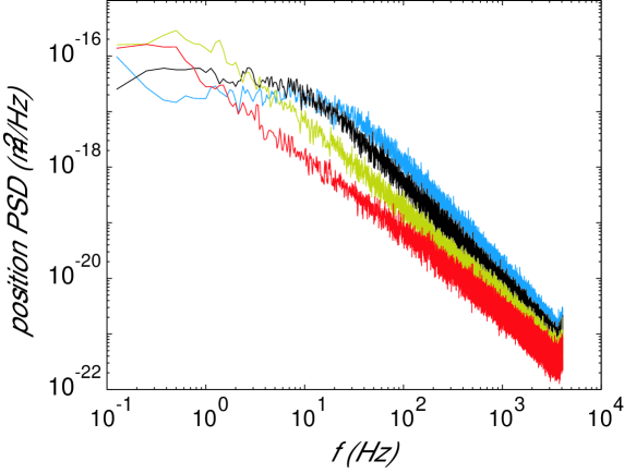
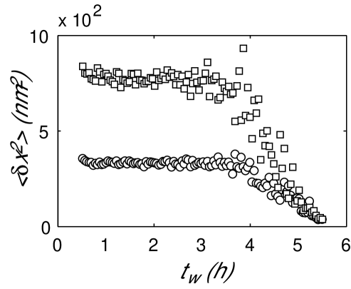
Figure 1: a) Spectra of the particle position fluctuations inside a Laponite solution at $2.3\%$ wt. The spectra has been measured for the trap stiffness $k_{1}=6.34$ pN/$\mu$m at various ageing times: from right to left $t_{w}=30$, $110$, $190$ and $270$ minutes. b) Evolution of $\left<\delta x^{2}\right>$ with $t_{w}$ for both stiffness, $k_{1}=6.34$ pN/$\mu$m ($\circ$) and $k_{2}=14.4$ pN/$\mu$m, ($\square$). The variances have been measured on a time window of $\tau=61$s

We find that $T_{eff}$ is constant at the beginning and is very close to $T_{bath}=294$ K, then when the jamming occurs, that is when $K_{Lap}$ increases, it becomes more scattered without any clear increase with $t_{w}$, contrary to Ref. [4]. We now make several remarks. First, we point out that the uncertainty of their results are underestimated. The error bars in Fig. 2a) are here evaluated from the standard deviation of the variance using Eq. 2 in Ref [4] at the time $t_{w}$. Although they are small for short time $t_{w}$, ($\Delta T_{eff}/T_{eff}\leq 10\%$), they increase for large $t_{w}$. This is a consequence of the increase of variabilities of $\left<\delta x_{i}^{2}\right>$ as the colloidal glass forms. This point is not discussed in in Ref. [4] and we think that the measurement errors are of the same order or larger than the observed effect. The results depend on the length of the analyzing time window and the use of the principle of energy equipartition becomes questionable for the following reasons.

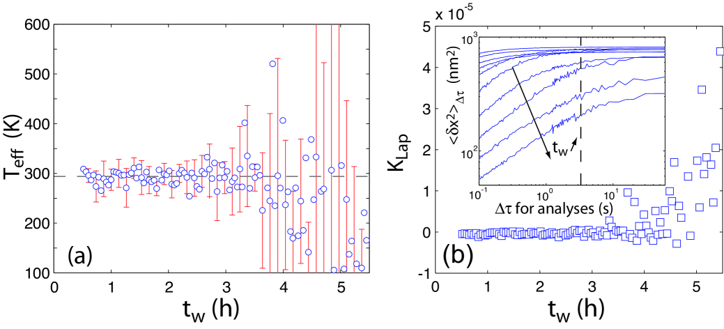
Figure 2: a) Evolution of the effective temperature with aging time for the data of Fig. 1 $k_{1}=6.34$ pN/$\mu$m, $k_{2}=14.4$ pN/$\mu$m, 2.3% wt of Laponite and 1 $\mu$m glass bead. The error bars are computed from the statistical error of $\left<\delta x_{i}^{2}\right>$ at the time $t_{w}$. b) Evolution of the stiffness of the Laponite with ageing time. Inset: Evolution of $\left<\delta x^{2}\right>_{\Delta\tau}$ for $k_{1}$ as a function of the duration $\Delta\tau$ of the samples for different aging times : $t_{w}=30$, $57$, $83$, $110$, $137$, $163$, $190$, $217$, $243$ and $270$ minutes.

First, these analyzing windows cannot be made too large because the viscoelastic properties of Laponite evolve as a function of time. Second, the corner frequency of the global trap (optical trap and gel), the ratio of the trap stiffness to viscosity, decreases continuously mainly because of the increase of viscosity. At the end of the experiment, the power spectrum density of the displacement of the bead shows that the corner frequency is lower than $0.1$ Hz. We thus observe long lived fluctuations, which could not be taken into account with short measuring times. This problem is shown on Fig. 2b). We split our data into equal time duration $\Delta\tau$, compute the variance and average the results of all samples. The dotted line represents the duration 3.3 s chosen in [4]. At the beginning of the experiment, the variance of the displacement is constant for any reasonable durations of measurement. However, we clearly see that this method produces an underestimate of $\left<\delta x^{2}\right>$ for long aging times, specially when the viscoelasticity of the gel becomes important. Long lived fluctuations are then ignored.

3.2 Passive rheology

This new method, using Kramers-Kronig relation, allows us to test the dependence of the effective temperature on the frequency. The figure 3a) shows the real part of $G$, which corresponds to the global elastic modulus of the gel and of the laser, for both trap stiffness. This numerical method is very sensitive to the spectrum. Thus, before computing the elastic modulus, we average the spectrum to obtain smooth curves. The uncertainties would then misplace the curve rather than produce a noisy curve. The increase with time is consistent with the increase of the strength of the gel. The elastic behavior of the Laponite is also more pronounced at high frequency. The last decrease of the curves at very high frequencies is due to the numerical method. Indeed, the frequency cutoff should be set at least a decade below the frequency of the data acquisition: data above 200 Hz is not reliable. We see that the curves of each stiffness are well separated except at the end of the measurement, where the results are not accurate due to the large difference between the optical stiffness and the Laponite stiffness.

From these data, we compute the ratio of the effective temperature to the bath temperature along the ageing process. These results are shown on Fig. 3b) for three different frequencies ($f=1$ Hz, 10 Hz and 100 Hz). We first note that the three curves are almost identical. This means that the effective temperature does not depends on the frequency. Second, the temperature ratio is close to 1. The dispersion of the data is rather small at early times and again increases when the stiffness of the gel overcomes those of the optical trap. This comes from the uncertainties on the elastic modulus which become larger than the difference between the two curves. This dispersion may also give, for very long time, negative temperatures, not shown in Fig. 3b) which is an expanded view. Even if this method is here less accurate than the previous one, it allows us to verify that the effective temperature is the same for all frequencies.

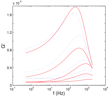
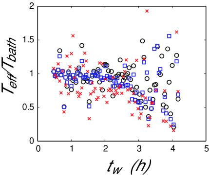
Figure 3: a) Evolution of $G^{\prime}$ (the global elastic modulus) as a function of frequency for both trap stiffnesses, $k_{1}=7.47$ pN/$\mu$m (solid lines), $k_{2}=16.7$ pN/$\mu$m (dashed lines) and for increasing ageing time: $t_{w}=30$ min, $90$ min, $140$min, $190$ min and $240$ min (1.2% wt of Laponite, 2 $\mu$m glass bead and ionic strength I=5 10^-3 mol.L^-1). b) Evolution of the ration $T_{eff}/T_{bath}$ with ageing time ($t_{w}$) for different frequencies (f=1 Hz $\square$, 10 Hz $\circ$ and 100 Hz $\times$)).

4 Conclusion

Finally, a remark has to be made concerning the mean position of the bead during aging. When the stiffness of the gel becomes comparable to the optical one, the bead starts to move away from the centre the optical trap. We observe a drift of the bead position at long time, which could lead to the escape of the bead. Moreover we have performed simultaneous measurements with a multiple trap using a fast camera showing that at very long $t_{w}$ the mean trajectories of beads separated by 7 $\mu$m are almost identical. This proves that one must pay attention when interpreting such measurements, specially on the duration of measurements. We also have seen that the way the sample is sealed can accelerate the formation of the gel and the drift of the bead by changing the chemical properties in the small sample. We have used different types of cell, Laponite concentrations, bead sizes, stiffness of the optical trap. In each case we do not find any increase of the effective temperature.

In conclusion, our results show no increase of $T_{eff}$ in Laponite and are in agreement with those of Jabbari-Farouji [5], who measured fluctuations and responses of the bead displacement in Laponite over a wide range of frequency and found that $T_{eff}$ is equal to the bath temperature.

5 Acknowledgement

This work has been partially supported by ANR-05-BLAN-0105-01.

References

- [1] L. Cugliandolo, J. Kurchan and L. Peliti, Phys. Rev. E, 55(4), (1997), pp. 3898 - 3914.
- [2] L. Bellon & S. Ciliberto, Physica D, 168 (2002), 325.
- [3] B. Abou & F. Gallet, Phys. Rev. Lett. 93 (16), (2006), 160603.
- [4] N. Greinert, T. Wood & P. Bartlett, Phys. Rev. Lett. 97 (2006), 265702.
- [5] S. Jabbari-Farouji et al.Phys. Rev. Lett. 98 (2007), 108302.
- [6] H. Tanaka, J. Meunier, D.Bonn Phys. Rev 69 (2004) 031404.
- [7] B. Schnurr, F. Gittes, F.C. MacKintosh, C.F. Schmidt, Macromolecules 30 (1997), 7781 .