Critical Behavior of Ferromagnetic Ising Model on Triangular Lattice

Abstract

We apply a new updating algorithm scheme to investigate the critical behavior of the two-dimensional ferromagnetic Ising model on a triangular lattice with nearest neighbour interactions. The transition is examined by generating accurate data for large lattices with $L=8,10,12,15,20,25,30,40,50$. The spin updating algorithm we employ has the advantages of both metropolis and single-update methods. Our study indicates that the transition to be continuous at $T_{c}=3.6403(2)$. A convincing finite-size scaling analysis of the model yield $\nu=0.9995(21)$, $\beta/\nu=0.12400(18)$, $\gamma/\nu=1.75223(22)$, $\gamma^{\prime}/\nu=1.7555(22)$, $\alpha/\nu=0.00077(420)$ (scaling) and $\alpha/\nu=0.0010(42)$(hyperscaling) respectively. Estimates of present scheme yield accurate estimates for all critical exponents than those obtained with Monte Carlo methods and show an excellent agreement with their well-established predicted values.

I Introduction

Ising Model on triangular lattice, as an archetypical example of a frustrated system, was initially studied by Wannier Wannier-1950-PR and Newll Newell-1950-PR . The triangular Ising model has attracted much attention and because of its remarkable properties it has a long history of investigation. No exact solution is available in two dimensions in an arbitrary magnetic field. Hence, simulations of the Ising model are essential. Monte Carlo simulation methods have been widely using techniques to update the spins of the system and to study the Ising model on triangular lattice to obtain numerical solutions.

A number of Monte Carlo methods based on Metropolis algorithms Metropolis-1953-J.Chem.Phys have been applied to the model in the past with somewhat mixed results. A classical Monte Carlo using Metropolis algorithm runs into difficulties on large lattice sizes due to critical slowing down and rapid increase in correlation time. Because of these reasons it is difficult to obtain meaningful results on larger lattice sizes. A cluster technique, which uses multi-cluster algorithm, was pioneered by Swendsen and Wang Swendsen-1987-PRL . Their method demonstrated its validity and efficiency for the Potts model successfully. Similar ideas have been pursued by Wolff Wolff-1989-PRL who proposed single-cluster algorithm, a nonlocal updating technique based on multiple-cluster algorithm but more efficient and easily applicable to achieve the meaningful results. Both of these cluster algorithms are very effective in reducing critical slowing down. But for the same system, one sweep of single-cluster or multiple-clusters take much more time than that of Metropolis algorithm, hence less effective for large lattice sizes. Very little has been done since then using these approaches on this model. Since large systems have the advantage of reducing finite-size effects, for this reason, we are forced to look yet again for an alternative approach.

In this study, we attempt to use a mixture of extend a single-cluster (multiple-cluster) and Metropolis algorithms to the Ising model in two-dimensions on triangular lattice. Applications of combined algorithm techniques have been extremely successful in lattice QCD Morningstar-1997-PRD ; Morningstar-1999-PRD ; Loan-2006-IJMPA ; Luo-2007-MPLA ; Loan08 ; Loan08a ; Loan08b ; Loan06c and have given rise to great optimism about the possibility of obtaining results relevant to continuum physics from Monte Carlo simulations of lattice version of the corresponding theory. As mentioned above, our aim is to use standard Monte Carlo techniques based on combined effect of single-cluster (multiple-cluster) and Metropolis algorithm to update the spins of the system and see whether useful results can be obtained. The values of the critical exponents are well established for this model in 2-dimensions and in order for our method to be considered successful, it must reproduce these well-established values. For this purpose, the critical exponents are computed by using the combined algorithm.

The rest of the paper is organised as follows: In Sec. II we discuss the Ising model in 2-dimensions in its lattice formulation. Here we describe the details of simulations and the methods used to extract the observables. We present and discuss our results in Sec. III. Our conclusions are given in Sec. IV

II Model and Simulation details

The Hamiltonian of the model is given by

$$H=-J\sum\limits_{<i,j>}S_{i}S_{j},$$ (1)

where $J$ is positive and denotes the strength of the ferromagnetic interaction, $S_{i}=\pm 1$ is the Ising spin variable, and $<i,j>$ restricts the summation to distinct pairs of nearest neighbors. The term on the right-hand side of Eq. 1 shows that the overall energy is lowered when neighbouring spins are aligned. This effect is mostly due to the Pauli exclusion principle. No such restriction applies if the spins are anti-parallel. The geometrical structure of the model is shown in Fig. 1. Periodic boundary conditions were employed during the simulations to reduce finite-size effects.

Figure 1: Triangular Ising net.

Configuration ensembles were generated using both mixture of Metropolis and single-cluster (multiple-cluster) methods on two dimensional triangular lattice of size $L=8-50$. We outline the procedure of single-cluster updating algorithm used to study the Ising model on triangular lattice below:

1. Choose a random lattice site x as the first point of cluster c to built.

2. Visit all sites directly connecting to x, and add them to the cluster c with probability $P(S_{x},S_{y})=1-\exp\{min[0,2KS_{x}S_{y}]\}$, where y is the nearest neighbor of site x and $K$ is the inverse temperature.

3. Continue iteratively in the same way for the newly adjoined sites until the process stops.

4. Flip the all sites of the cluster c.

5. Repeat(a), (b), (c) and (d) sufficient times.

We define a compound sweep as one single-cluster updating sweep following with five Metropolis updating sweeps. In our simulations, five compound sweeps were performed between measurements. We observed that Metropolis - single-cluster (multiple-cluster) and compound sweep updating techniques proved equally good for large ensembles. However, in case of the compound sweep technique the computational cost turned out to be far less. For this reason we adapted this technique in our simulations.

We generated $1\times 10^{7}$ ensembles at transition point for each lattice size to performed the finite-size analysis. High statistics could help us to obtain a more accurate result. Since the ensembles were generated by Monte Carlo method, they were not completely uncorrelated. The Jackknife procedure was employed because it took the autocorrelation between the ensembles into account and provided an improved estimate of the mean values and errors.

III Results and discussion

From the fluctuation dissipation theorem, the heat capacity ($C$) is the derivative of the energy with respect to temperature and has the form

$$C=\frac{<E^{2}>-<E>^{2}}{L^{2}T^{2}}.$$ (2)

For improved comparability among different system sizes, it is better to compute the heat capacity per spin which is displayed in in Fig. 2. Theoretical derivations suggest that the heat capacity should behave like $\log\mid T-T_{c}\mid$ near the critical temperature. We notice a progressive steepening of the peak as the lattice size increases, which illustrates a more apparent phase transition. Note that due to finite size effects, the peak is flattened and moved to the right. Our interest is to look for such a transition point and investigate the critical phenomena associated with the transition using finite-size scaling method Fisher-1972-PRL ; Landau-1976-PRB ; Binder-1981-Z.Phys.B

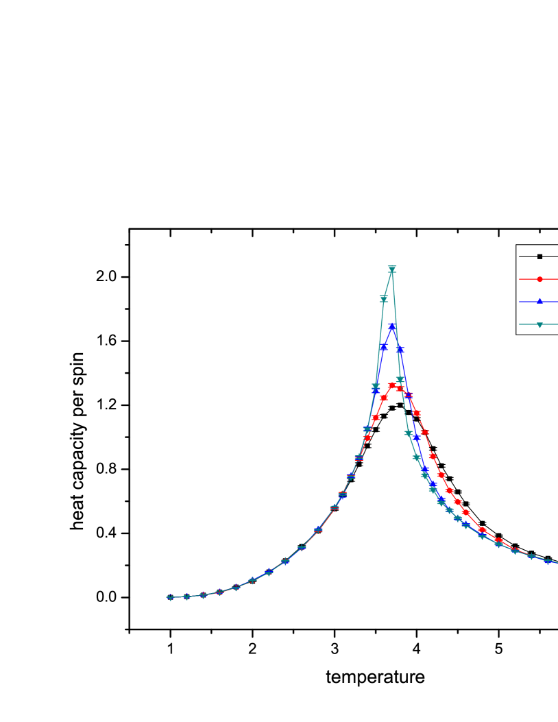
Figure 2: Plot showing the differing results of the heat capacity with respect to temperature for varying lattice size, $L\times L$.

III.1 Estimation of the transition temperatures

The fourth-order magnetic cumulant $U_{L}$, which is used to estimate the transition temperature, is defined by the following expression Binder-1981-Z.Phys.B :

$$U(T,L)=1-\frac{<m^{4}(T,L)>}{3<m^{2}(T,L)>^{2}},$$ (3)

where $<m^{k}(T,L)>$ is the thermodynamic average value of the $k$th power of the magnetic order parameter per spin for the lattice of size $L$ with temperature $T$. The variation of $U(T,L)$, for a given size $L$, with the temperature is illustrated in Fig. 3. To determinate the temperature $T_{c}(L,L^{\prime})$, we make use of the condition Binder-1981-Z.Phys.B ; Peczak-1991-PRB

$$\left.\frac{U(T,L^{\prime})}{U(T,L)}\right|_{T=T_{c}(L,L^{\prime})}=1,$$ (4)

where $L^{\prime}$ and $L$ are two different lattice sizes. Thus we can determine $T_{c}(L,L^{\prime})$ by locating the interaction of these curves - the so called “cumulant crossing”.

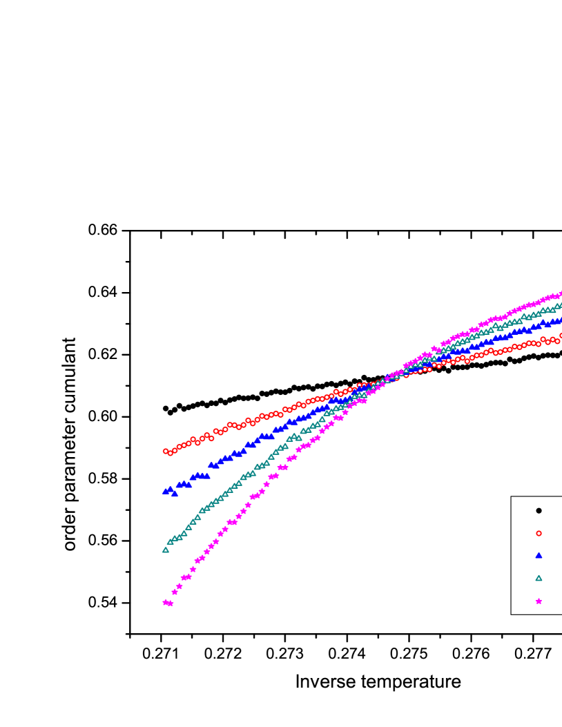
Figure 3: The fourth-order magnetic parameter cumulant plotted as a function of inverse temperature for several lattice sizes.

Fig. 4 shows the results for $T_{c}(L,L^{\prime})$ plotted as a function of the ratio $\ln^{-1}(L^{\prime}/L)$. Keeping $L$ fixed, linear extrapolation is performed to obtain $T_{c}(L,\infty)$ which corresponds to the critical temperature of lattice size $L$. Results of the extrapolations for $8\leq L\leq 15$ agree quite well within the errors. The transition temperature for the infinite lattice is thus estimated as $T_{c}=3.6403(2)$, which is much close to the exact value $4/\ln 3$.

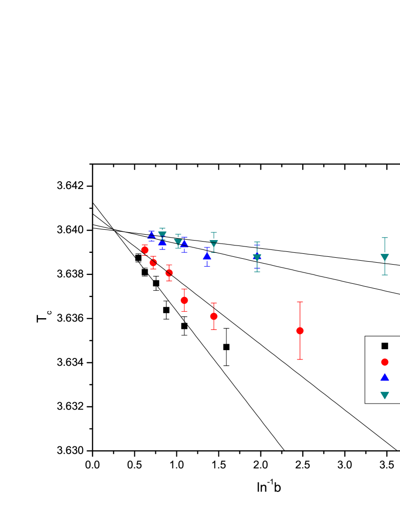
Figure 4: Estimates for $T_{c}$ plotted vs inverse logarithm of the scale factor $b=L^{\prime}/L$ for serval lattice sizes.

III.2 Order of the transition

A better way to identify the order of the transition is the internal-energy cumulant Binder-1981-PRL ; Binder-1984-PRB ; Challa-1986-PRB ; Ferrenberg-1988-PRL ; Billoire-1990-PRB ; Rastelli-2005-PRB defined by

$$V(T,L)=1-\frac{<E^{4}(T,L)>}{3<E^{2}(T,L)>^{2}},$$ (5)

where $<E^{k}(T,L)>$ is the thermodynamic average value of $k$th power of internal energy for the lattice of size $L$ with temperature $T$. $V(T,L)$ is a useful quantity since its behavior at a continue phase transition is quite different from that at a first order transition. This variable has a minimum (near the critical point), and in the limit $L\rightarrow\infty$ achieves the value $V^{*}=\frac{2}{3}$ for a continuous transition, whereas $V^{*}<\frac{2}{3}$ is expected in the case of a first-order transition. Plots of $V(T,L)$ versus temperature for several lattice sizes are shown in Fig. 5. The graphs indicate that the transition is not first-order since the energy culumant $V(T,L)$ does not peak near the critical temperature. This has also been observed in various other studies Challa-1986-PRB ; Billoire-1990-PRB ; Rastelli-2005-PRB .

Fig. 6 shows the order parameter cumulant $U(T,L)$ as a function of temperature for serval lattice sizes. In contrast with obtaining a negative minimum value in first order transition, $U(T,L)$ drops from $2/3$ for $T<T_{c}$ to 0 for $T>T_{c}$. This is in agreement with the continuous transition Binder-1981-PRL .

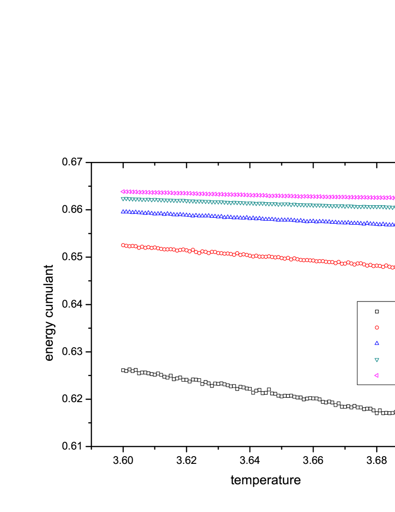
Figure 5: Plots of energy cumulant with respect to temperature for serval lattice sizes.

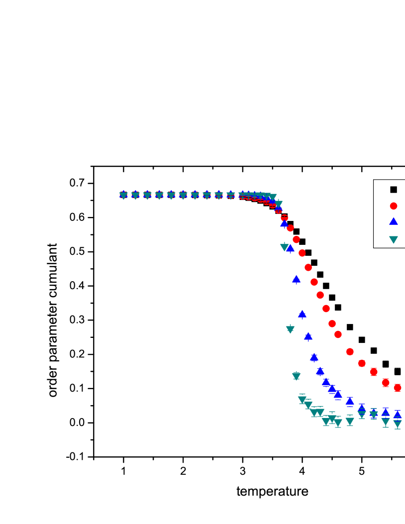
Figure 6: plots of order parameter cumulant with respect to temperature for serval lattice sizes.

Since the magnetic susceptibility $\chi$ scales as $L^{d}$ for a discontinuous transition and as $L^{\gamma/\nu}$ for a continuous one Bunker-1993-PRB , we can also determine the transition order by $\chi$’s scaling behaviors. As discussed below, we find that $\chi$ scales as $L^{1.75223}$ for $T<T_{c}$ and as $L^{1.7555}$ for $T>T_{c}$, but not as $L^{2}$. Thus we can conclude that the transition is continuous.

III.3 Estimation of the critical exponents

To get an estimation for the critical exponents, finite-size scaling relations at critical point are used. For this purpose, we extract the critical exponents, which are related to specific heat, the order parameter, and the susceptibility, from our simulation data at $T_{c}(\infty)$ by using finite-size analysis Fisher-1972-PRL ; Landau-1976-PRB ; Binder-1981-Z.Phys.B .

First we extract $\nu$ from $dU/dK$ which obey the following relation

$$\frac{dU}{dK}\sim L^{1/\nu},$$ (6)

Finite-difference derivative method can be used to determinate $dU/dK$, but it is rather a poor choice since the results are highly sensitively to the interval of the linear approximation. To obtain a precise result of the critical exponent $\nu$, one can write the derivative of $U$ with respect to $K$ as

$$\frac{dU}{dK} = \frac{1}{3<m^{2}>^{2}}\left[<m^{4}><E>-2\frac{<m^{4}><m^{2}E>}{<m^{2}>}\right.$$ (7)

$$\left.+<m^{4}E>\right]$$

$$= <\frac{m^{4}(<E>+E)}{3<m^{2}>^{2}}>-<\frac{2m^{2}E<m^{4}>}{3<m^{2}>^{3}}>.$$

The plot of $\ln(dU/dK)$ versus $\ln L$ is shown in Figure 7. The slope of the straight line obtained from the log-log plot of the scaling relation corresponding to this quantity gives the correlation length exponent $\nu=0.9995(21)$, which is slightly different from the theoretical value. Since the critical properties of $\ln(dU/dK)$ have a large lattice size dependence Bunker-1993-PRB , we could also extract the value of $\nu$ from other observables, which are defined as following Ferrenberg-1991-PRB ; Bunker-1993-PRB ; Chen-1993-PRB :

$$V_{1} = \ln\left[\frac{d\ln<m>}{dK}\right]=\ln\left[<E>-\frac{<mE>}{<m>}\right]$$ (8)

$$= \ln\langle\frac{E(<m>-m)}{<m>}\rangle,$$

$$V_{2} = \ln\left[\frac{d\ln<m^{2}>}{dK}\right]=\ln\langle\frac{E(<m^{2}>-m^{2})}{<m^{2}>}\rangle,$$ (9)

$$V_{3} = 2[m]-[m^{2}],$$ (10)

$$V_{4} = 3[m^{2}]-2[m^{3}],$$ (11)

where

$$[m^{n}] = \ln\frac{\partial<m^{n}>}{\partial K}$$ (12)

$$= \ln(<E><m^{n}>-<m^{n}E>)$$

$$= \ln<E(<m^{n}>-m^{n})>.$$

The curves show a smooth behavior and linear fitting of the data is adopted. We found the slopes of the straight lines of $V_{i}$, with $i=1,2,3,4$, are very close to that of $\ln(dU/dK)$, as illustrated in Fig. 7.

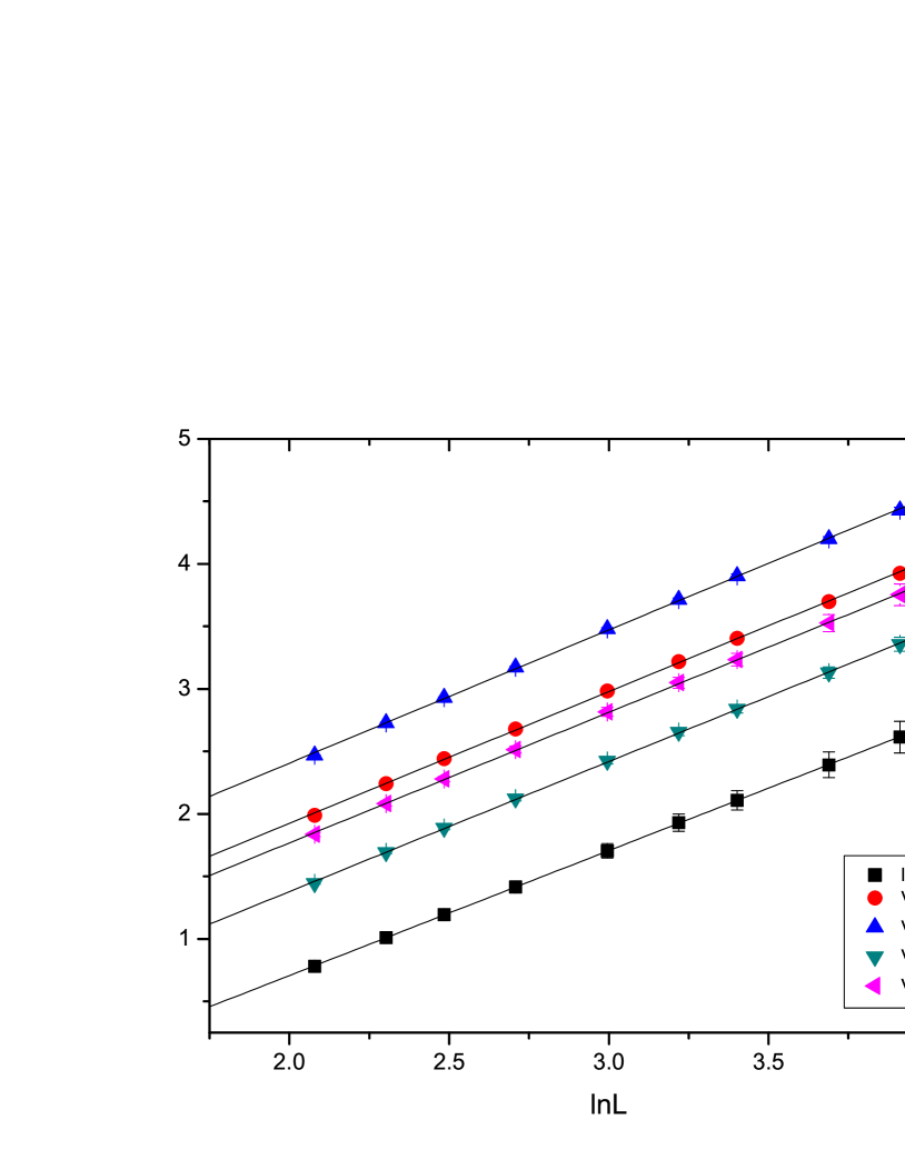
Figure 7: The critical exponent $\nu$ is determined from the slope of $\ln(dU_{L}/dK)$ and $V_{i}$ vs $\ln L$ at $T=3.6403$. Linear fittings result in $\nu=0.9995(21)$.

Figure 8 displays the double-logarithmic plot of the magnetization at transition point as a function of $L$. According to the standard theory of finite-size scaling, at $T_{c}$ the magnetization per spin should obey the relation

$$m\sim L^{-\beta/\nu},$$ (13)

for sufficiently large lattice size. The data falls nicely on a linear curve and the slope of the curve gives an estimate for the ratio of critical exponents $\beta/\nu=0.12400(18)$. Using our estimate of $\nu=0.9995(21)$, we get the critical exponent of magnetization $\beta=0.12394(32)$.

Figure 8: Plot of $\ln m$ as a function of $\ln L$ at $T=3.6403$.

On finite lattices, the magnetic susceptibility per spin is given byBinder-1969-Z.Phys. ; Peczak-1991-PRB

$$\chi=(L^{2}/T)<m^{2}>$$ (14)

for $T>T_{c}$ and

$$\chi^{\prime}=(L^{2}/T)(<m^{2}>-<m>^{2})$$ (15)

for $T<T_{c}$, and satisfy

$$\chi\sim L^{\gamma/\nu},\hskip 28.45274pt\chi^{\prime}\sim L^{\gamma^{\prime}/\nu}.$$ (16)

As another estimation, we compute the magnetic susceptibility per spin by examining log-log plot shown in Fig. 9 of $\chi$ and $\chi^{\prime}$ versus $L$ at the transition point. The data displays a smooth scaling behaviour. The slope of the linear fit to the data gives estimates of $\gamma/\nu=1.75223(22)$ and $\gamma^{\prime}/\nu=1.7555(22)$, respectively. With our estimated values $\nu=0.9995(21)$, we obtain $\gamma=1.7514(37)$ and $\gamma^{\prime}=1.7546(43)$, respectively. These results agree rather well with the theoretical prediction.

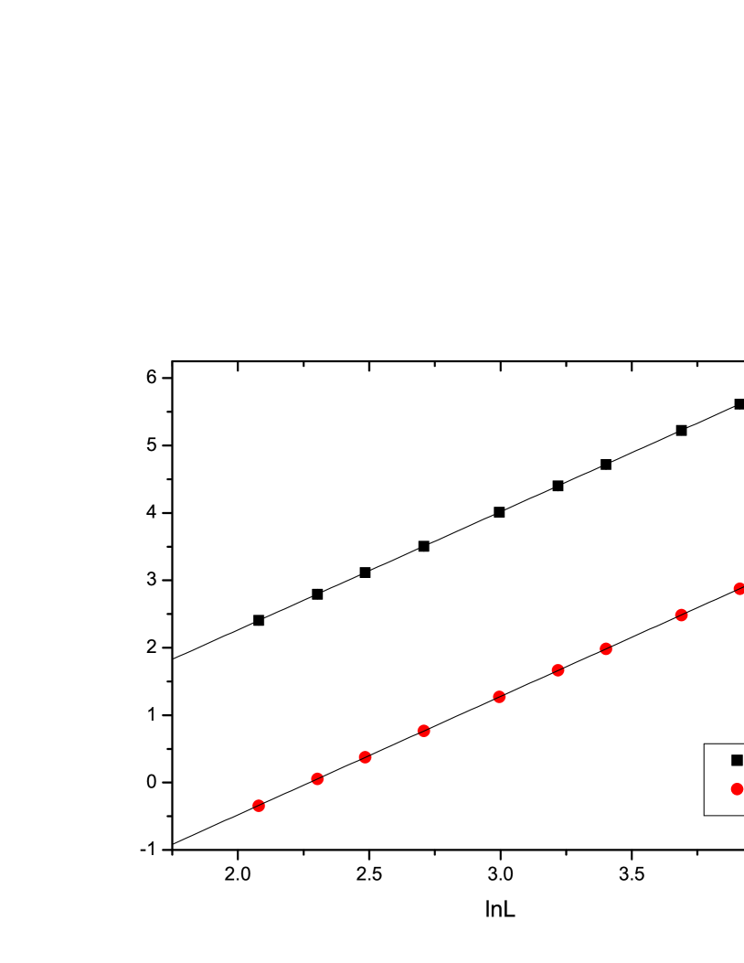
Figure 9: Plot of $\ln\chi$ and $\ln\chi^{\prime}$ vs $\ln L$ at $T=3.6403$.

With three critical exponents $\nu$, $\gamma$, $\beta$ determined, the fourth exponent $\alpha$ is estimated using scaling law

$$2\beta+\alpha+\gamma=2.$$ (17)

This yields $\alpha/\nu=0.00077(420)$ and $\alpha=0.00077(420)$ for $\gamma/\nu=1.75222(22)$, $\alpha/\nu=-0.0025(47)$ and $\alpha=-0.0025(47)$ for $\gamma^{\prime}/\nu=1.7555(22)$ respectively. We can also estimate $\alpha$ from hyperscaling relation

$$d\nu+\alpha=2,$$ (18)

where $d=2$ is dimension of the system. It gives a result $\alpha=0.0010(42)$ and $\alpha/\nu=0.0010(42)$, which is consistent with that given by scaling law.

Estimates of critical exponents from finite-size scaling at critical temperature $T_{c}$ are summerized in Table 1.

Table 1: Estimates of critical exponents

exponent	value	exact valueFisher-1967-Rep.Prog.Phys. ; Mon-1993-PRB
$\nu$	0.9995(21)	1
$\beta/\nu$	0.12400(18)	$1/8$
$\gamma/\nu$	1.75223(22)($T>T_{c}$)	$7/4$
$\gamma^{\prime}/\nu$	1.7555(22)($T<T_{c}$)	$7/4$
$\alpha/\nu$	0.00077(420)(by scaling)	0
$\alpha/\nu$	0.0010(42)(by hyperscaling)	0

To ensure the validity of our estimate of $\alpha$, we compare it with those obtained using the specific heat per spin from the fluctuations of the total energy. For a continuous transition it behaves as

$$C\simeq a+bL^{\alpha/\nu}.$$ (19)

Figure 10: Plot of heat capacity $C$ with respect to $L^{\alpha/\nu}$, where $\alpha/\nu=0.00077$ and $C$ is evaluated at $T_{c}=3.6403$.

Using $\alpha/\nu=0.00077(420)$ calculated above, the heat capacity at critical temperature is plotted as a function of $L^{0.00077}$ in Fig. 10. It was found that the evaluations of (17) and (19) yield results very consistent within statistical errors. We find the values are in good agreement with the theoretical ones. An over all error of about $0.1-0.8\%$ is estimated for the values of the critical exponents

IV Conclusions

We have obtained critical exponents for the Ising model with nearest-neighbour interactions on a triangular lattice by using a mixture of single-cluster and Metropolis algorithm in our simulations. The data are analysed according to the finite-size scaling theory. The idea of using extensions of mixed algorithm to estimate the critical exponents seems to supply a quite accurate route for their estimation. In conclusion, it can be stated that the compound update algorithm method with periodic boundary conditions reproduces with a high accuracy the critical properties of the model and confirms the prediction that first order transition is not supported by the finite size behavior of the system. Our results show that the several estimations for the critical exponents are in good agreement with their theoretical values. We stress that the present result for the exponent is better than previous estimates obtained by finite size scaling and Monte Carlo approach.

V Acknowledgements

This work was supported in part by Guangdong Natural Science Foundation(GDNSF) Grant No. 07300793. ML was supported in part by the Guangdong Ministry of Education. We would like to express our gratitude to the Theory Group at Sun Yat-Sen University for the access to its computing facility.

References

- (1) G. H. Wannier, Phys. Rev. 79, 357(1950).
- (2) G. F. Newell, Phys. Rev. 79, 876(1950).
- (3) N. Metropolis, A. W. Rosenbluth, M. N. Rosenbluth, A. H. Teller and E. Teller, J. Chem. Phys. 21, 1087(1953).
- (4) Robert H. Swendsen and Jian-Sheng Wang, Phys. Rev. Lett. 58, 86(1987).
- (5) Ulli Wolff, Phys. Rev. Lett. 62, 361(1989).
- (6) Colin J. Morningstar and Mike Peardon, Phys. Rev. D 56, 4043(1997).
- (7) Colin J. Morningstar and Mike Peardon, Phys. Rev. D 60:034509(1999).
- (8) Mushtaq Loan, Xiang-Qian Luo and Zhi-Huan Luo, Int. J. Mod. Phys. A, Vol. 21, Nos. 13&14(2006) 2905-2936.
- (9) Zhi-Huan Luo, Mushtaq Loan and Xiang-Qian Luo, Mod. Phys. Lett. A, Vol. 22, Nos. 7-10(2007) 591-597.
- (10) M. Loan, submitted to Phys. Lett. B.
- (11) M. Loan, Z-H Luo, and Y.Y. Lam, Eur. Phys. J. C 56 (2008).
- (12) M. Loan, Eur. Phys. J. C 54, 475 (2008).
- (13) M. Loan and Y. Ying, Prog. Theo. Phys. 116, 169 (2006).
- (14) Michael E. Fisher and Michael N. Barber, Phys. Rev. Lett. 28, 1516(1972).
- (15) D.P. Landau, Phys. Rev. B 14, 255(1976).
- (16) K. Binder, Z. Phys. B 43, 119(1981).
- (17) P. Peczak, Alan M. Ferrenberg and D. P. Landau, Phys. Rev. B 43, 6087(1991).
- (18) K. Binder, Phys. Rev. Lett. 47, 693(1981).
- (19) K. Binder and D. P. Landau, Phys. Rev. B 30, 1477(1984).
- (20) Murty S. S. Challa, D. P. Landau and K. Binder, Phys. Rev. B 34, 1841(1986).
- (21) Alan M. Ferrenberg and Robert H. Swendsen, Phys. Rev. Lett. 61, 2635(1988).
- (22) A. Billoire et al, Phys. Rev. B 42, 6743(1990).
- (23) E. Rastelli, S. Regina and A. Tassi, Phys. Rev. B 71, 174406(2005).
- (24) Alan M. Ferrenberg and D. P. Landau, Phys. Rev. B. 44, 5081(1991).
- (25) Alex Bunker, B. D. Gaulin and C. Kallin, Phys. Rev. B. 48, 15861(1993).
- (26) Kun Chen, Alan M. Ferrenberg and D. P. Landau, Phys. Rev. B. 48, 3249(1993).
- (27) K. Binder and H. Rauch, Z. Phys. 219, 201(1969).
- (28) M. E. Fisher, Rep. Prog. Phys. 30, 615(1967).
- (29) K. K. Mon, Phys. Rev. B. 47, 5497(1993).