Quantum chaos and its kinetic stage of evolution

Abstract

Usually reason of irreversibility in open quantum-mechanical system is interaction with a thermal bath, consisting form infinite number of degrees of freedom. Irreversibility in the system appears due to the averaging over all possible realizations of the environment states. But, in case of open quantum-mechanical system with few degrees of freedom situation is much more complicated. Should one still expect irreversibility, if external perturbation is just an adiabatic force without any random features? Problem is not clear yet. This is main question we address in this review paper. We prove that key point in the formation of irreversibility in chaotic quantum-mechanical systems with few degrees of freedom, is the complicated structure of energy spectrum. We shall consider quantum mechanical-system with parametrically dependent energy spectrum. In particular, we study energy spectrum of the Mathieu-Schrodinger equation. Structure of the spectrum is quite non-trivial, consists from the domains of non-degenerated and degenerated stats, separated from each other by branch points. Due to the modulation of the parameter, system will perform transitions from one domain to other one. For determination of eigenstates for each domain and transition probabilities between them, we utilize methods of abstract algebra. We shall show that peculiarity of parametrical dependence of energy terms, leads to the formation of mixed state and to the irreversibility, even for small number of levels involved into the process. This last statement is important. Meaning is that, we are going to investigate quantum chaos in essentially quantum domain.

In the second part of the paper, we will introduce concept of random quantum phase approximation. Then along with the methods of random matrix theory, we will use this assumption, for derivation of muster equation in the formal and mathematically strict way.

Content of the paper is based on our previous studies. However, in this review paper is included also some original material. This part mainly concerns to the discussion about possible experimental realization of theoretical concepts in the field of organic chemistry.

$\bf keywords:$ Statistical Physics, Quantum Chaos, Nonlinear Resonance, Open Quantum-Mechanical Systems.

$\bf{Introduction}$

The traditional notion of an area, where the laws of statistical physics are effective, consists of the assumption that the number of interacting particles is sufficiently large. However, a lot of examples of nonlinear systems with a small number of degrees of freedom, where chaotic motions occur, had become known by the end of last century Sagdeev ; Lichtenberg ; Alligood . A new stage in the development of notions about chaos and its origin appeared in the last two decades of the last century. It turned out that classical Hamiltonian near the separatrix of topologically different trajectories may experience a special kind of instability. Because of this instability various dynamic characteristics of the system randomly change with time. Such a property of the system that performs random motion is called dynamic stochasticity. Dynamic stochasticity is an internal property of the system and is not associated with the action of some a priory random forces.

Dynamic stochasticity appears due to the extreme sensitivity of nonlinear system with respect to the slightly change of initial conditions or systems parameters. On the other hand, even being chaotic, dynamic is still reversible. Irreversibility occurs only after averaging of the dynamic over small dispersion of initial data. Note that averaging is not formal mathematical procedure. It is essential from the physical point of view. Since dynamical description loses its sense due to local instability of phase trajectories. However not the existence of initial error is important but, what kind of consequences it has. In case of linear system, this influence is negligible. So one can always assume that initial data for linear system is defined with the absolute accuracy. But in case of nonlinear systems, even small unavoidable error should be taken into account. This leads to the necessity of using concepts of statistical physics. As a result, analytical description becomes much more complicated. All above mentioned was concerned to the classical case. What is really happening in quantum case? Should one still expect non-reversibility in quantum case? The question is that as opposite to the classical case, quantum equation of motion is linear. Of course, things are more or less clear in case of open quantum systems interacting with the thermostat. If so, then, irreversibility appears owing to the averaging of systems dynamics over all possible realizations of environment states. Due to this, one can use standard formalism, and from the Liouville-von Neumann equation, deduce irreversible in time muster equation, for the reduced density matrix Honggi . But how does the irreversibility occur in quantum systems with few degrees of freedom This is main question we address in this review paper.

Usually quantum irreversibility is quantified by the fidelity. Introduced by Peres Peres , this concept works pretty well and is especially convenient for the study of problems like quantum chaotic billiards Jacquod . On the other hand, disadvantage is that obtaining of analytical results not always is possible and large computational resources usually are needed.

In this paper, we offer alternative analytical method for the study of problem of quantum irreversibility. Our concept is based on the features of the energy spectrum of chaotic quantum systems. Peculiarity of energy spectrum of chaotic quantum systems is well-known long ago Haake . Random Matrix Theory (RMT) presumes eigenvalues of chaotic systems to be randomly distributed. Number of levels also should be quite large. In order to deduce muster equation for time dependent chaotic system, we will utilize methods of RMT in the second part of this paper. However, what we want to discuses in the first part is completely different. The key point is that, study of quantum chaos as a rule is focused on the semi-classical domain. We mean not only Gutzwiller’s semi-classical path integration method Stockman , but also RMT. Since the RMT, in somehow implies semi-classical limit. At least implicitly, due to the large number of levels included into process.

In the first part of our paper, we shall consider chaotic quantum-mechanical system with few levels included into process. In spite of this, feature of the energy levels leads to the irreversibility.

Paper is organized as follows:

In the first part we shall consider quantum mechanical-system with parametrically dependent energy spectrum. This parametrical dependence is quite non-trivial, contains domains of non-degenerated and degenerated stats separated from each other by branch points. Namely energy spectrum of our system is given in terms of Mathieu characteristics. Due to the modulation in time of the parameter, system will perform transitions from one domain to other one. For determination of eigenstates for each domain and transition probabilities between them, we utilize methods of abstract algebra. We shall show that peculiarity of parametrical dependence of energy terms, leads to the formation of mixed state and to the irreversibility, even for small number of levels involved into the process. So this part may be considered as an attempt to study quantum chaos in the essentially quantum domain. This study is based on our previous papers Ugulava ; Chotorlishvili ; Nickoladze ; Gvarjaladze . In addition, in the present paper, we will discuss in details possible experimental realizations and applications of the theoretical concepts in the organic chemistry and polyatomic organic molecules.

In the second part of the paper, we will introduce concept of random quantum phase approximation. Then we will use this assumption, for derivation of muster equation in the most formal and mathematically strict way.

I Quantum Pendulum

I.1 Universal Hamiltonian

Let us present the atom as a nonlinear oscillator under the action of the variable monochromatic field. Then the Hamiltonian of the system atom + field is of the form:

$$H(x,p,t)=H_{0}(x,p)+H_{NL}(x)+\varepsilon V(x,t),$$ (1)

where

$$H_{0}=1/2(\frac{p^{2}}{m}+\omega_{0}^{2}mx^{2}),~{}~{}H_{NL}=\beta x^{3}+\gamma x^{4}+\ldots,$$ (2)

$$V(x,t)=V_{0}x\cos\Omega t,~{}\varepsilon V_{0}=\frac{e}{m}f_{0},~{}\varepsilon\ll 1.$$ (3)

Here $x$ and $p$ are coordinate and the impulse of the particle (electron), $\omega_{0}$ is the frequency of oscillations, $\beta$ and $\gamma$ are coefficients of nonlinearity, $m$ and $e$ are the mass and charge of the particle, $f_{0}$ is the amplitude of the variable field. Having made passage to the variables of action-angle $I,\theta$ with the help of transformation $x=(2I/m\omega_{0})^{1/2}\cos\theta,p=-(2Im\omega_{0})^{1/2}\sin\theta,$ supposing resonance condition $\Omega\approx\omega_{0}$ is realized and averaging with respect to the fast phase $\theta$, one can obtain:

$$H=H_{0}(I)+\varepsilon V(I)\cos\varphi,$$

where

$$H_{0}(I)=\omega_{0}I+H_{NL},~{}~{}H_{NL}(I)=\frac{3\pi}{4}(\frac{I}{m\omega^{2}_{0}})^{2}\gamma$$ (4)

$$\varphi=\theta-\omega t,~{}~{}\varepsilon V(I)=\sqrt{I/m\omega_{0}}V_{0}.$$ (5)

The role of nonlinear frequency plays $(dH_{0}/dI)=\omega_{0}+\omega_{NL}(I)$ where $\omega_{NL}(I)=(3\pi/2)(I\gamma/m\omega^{2}_{0})$. Now suppose that nonlinear resonance condition $\omega_{0}+\omega_{NL}(I_{0})=\Omega$ is fulfilled for action $I=I_{0}$. It is easy to show Sagdeev , that for a small deviation of action from the resonance value $\Delta I\equiv I-I_{0}~{}(\Delta I\ll I_{0})$ after the power series expansion, if the condition of moderate nonlinearity is just $\mu\ll 1/\varepsilon$, where

$$\mu\equiv\omega_{NL}(I/\omega_{NL}(I))|_{I=I_{0}},~{}~{}\omega_{NL}=(d\omega_{NL}(I)/dI)|_{I=I_{0}},$$

for Hamiltonian we obtain:

$$H=\frac{\omega_{NL}}{2}(\Delta I)^{2}+\varepsilon V(I_{0})\cos\varphi.$$ (6)

As usual (6) is called universal Hamiltonian. Let us notice that Hamiltonian $H$ is the Hamiltonian of pendulum, where $I/\omega_{NL}$ plays the role of mass, $\Delta I$ plays the role of the pulse and $V(I_{0})$ plays the role of potential energy. If in (6) $\Delta I$ is substituted by the appropriate operator $\Delta I\rightarrow-i\hbar\partial/\partial\varphi$, one can obtain the universal Hamiltonian in the quantum form

$$H=-\frac{\hbar^{2}\omega^{\prime}}{2}\frac{\partial^{2}}{\partial\varphi^{2}}+V\cos\varphi.$$ (7)

With the help of (7) it is possible to explore quantum properties of motion for the nonlinear resonance.

Having written the stationary Schrodinger equations

$$\hat{H}\psi_{n}=E_{n}\psi_{n}$$ (8)

for the Hamiltonian (7), we get

$$\frac{\partial^{2}\psi_{n}}{\partial\varphi^{2}}+(E_{n}-V(l,\varphi))\psi_{n}=0,$$ (9)

$$V(l,\varphi)=2l\cos 2\varphi$$

where the dimensionless quantities are introduced

$$E_{n}\rightarrow\frac{8E_{n}}{\hbar^{2}\omega^{\prime}},~{}l\rightarrow\frac{4V}{\hbar^{2}\omega^{\prime}}$$ (10)

and the replacement $\varphi\rightarrow 2\varphi$ is done.

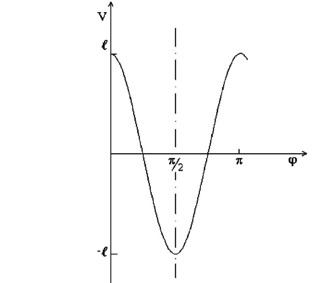
Figure 1: The dependence of the energy of interaction $V$ from the phase.

The interaction has the following properties of the symmetry: $1.V(\varphi)=V(-\varphi),~{}2.V(\varphi)=V(\pi+\varphi),~{}3.V(\frac{\pi}{2}+\varphi)=V(\frac{\pi}{2}-\varphi).$ G.M.Zaslavsky and G.P.Berman [8] were the first who considered the equation of the Mathieu-Schrodinger for the quantum description of the nonlinear resonance in the approximation of moderate nonlinearity. They studied the case of quasi-classical approximation $\Delta I\gg\hbar$ for both variables $I_{0}$ and $\Delta I$. In this review we investigate the equation of the Mathieu - Schrodinger in essentially quantum area.

I.2 Periodical solution of Mathieu - Schrodinger equations

We content ourselves with only even and odd solutions with respect to $\varphi$ of equation of the Mathieu - Schrodinger (9). Those solutions have $n$ zeroes in the interval $0\leq\varphi\leq\pi$. Eigenfunctions $\psi_{n}$ can be recorded with the help of the Mathieu functions [9,10]: even $ce_{n}(\varphi,l)$ and odd $se_{n}(\varphi,l)$. Appropriate eigenvalues are usually designated by $a_{n}(l)$ and $b(l)$. For simplicity below sometimes we omit the argument $l$ and write $ce_{n}(\varphi),~{}se_{n}(\varphi),~{}a_{n},~{}b_{n}.$ Mathieu functions are eigenfunctions of the problem of Sturm-Liouville for the equation (9) for the boundary conditions

$$\psi(0)=\psi(\pi)=0,~{}~{}~{}for~{}~{}~{}se_{n}(\varphi)$$

$$\frac{d\psi}{d\varphi}(0)=\frac{d\psi}{d\varphi}(\pi)=0,~{}~{}~{}for~{}~{}~{}ce_{n}(\varphi).$$ (11)

From the general theory of the Sturm-Liouville it follows, that for arbitrary $n=1,2,\dots$ there exists eigenfunction $se_{n}(\varphi)$ and for each $n=0,1,2,\dots$ determined eigenfunction $ce_{n}(\varphi)$. The definition of the Mathieu function must be supplemented with the choice of the arbitrary constant so that the conditions were fulfilled:

$$ce_{n}(0,l)>0,~{}~{}~{}\frac{1}{\pi}\int_{0}^{2\pi}ce_{n}^{2}(\varphi,l)d\varphi=1,$$

$$\frac{dse_{n}}{d\varphi}(0,l)>0,~{}~{}~{}\frac{1}{\pi}\int_{0}^{2\pi}se_{n}^{2}(\varphi,l)d\varphi=1.$$ (12)

If $\psi(\varphi)\equiv G(\varphi)$ means either $ce_{n}(\varphi)$ or $se_{n}(\varphi)$, then $G(\varphi)$ and $G(\pi-\varphi)$ satisfy the same equation (9) and the same boundary conditions (11). Therefore these functions differ from each other only by the constants. Hence, $G(\varphi)$ is even or odd function with respect to $\pi/2-\varphi$. Taking this into account, two functions (11) break up into four Mathieu functions:

$$\psi(0)=\psi(\pi/2)=0,~{}~{}G(\varphi)=se_{2m+2}(\varphi),~{}~{}phase~{}~{}\pi,$$

$$\psi(0)=\frac{d\psi}{d\varphi}(\pi/2)=0,~{}~{}G(\varphi)=se_{2m+1}(\varphi),~{}~{}phase~{}~{}2\pi,$$

$$\frac{d\psi}{d\varphi}(0)=\psi(\pi/2)=0,~{}~{}G(\varphi)=ce_{2m+1}(\varphi),~{}~{}phase~{}~{}2\pi,$$

$$\frac{d\psi}{d\varphi}(0)=\frac{d\psi}{d\varphi}(\pi/2)=0,~{}~{}G(\varphi)=ce_{2m}(\varphi),~{}~{}phase~{}~{}\pi.$$ (13)

For arbitrary $m=0,1,2,\dots$ there is one eigenfunction for each of four boundary conditions and $m$ equal to the number of zeroes in the interval $0<\varphi<\pi/2$. The functions (13) represent a complete system of eigenfunctions of the equation (9).

I.3 Symmetries of the equations of Mathieu-Schrodinger

The properties of symmetry of the Mathieu-Schrodinger equation can be presented in Table 1 Bateman .

As is known, group theory makes it possible to find important consequences, following from the symmetry of the object under study. Below, with the aid of group theory we will establish the presence (or absence) of degeneracy in the eigen spectrum of the Mathieu-Schrodinger equation and a form of corresponding wave functions By immediate check it is easy to convince, that four elements of transformation

$$G(\varphi\rightarrow-\varphi)=a,~{}~{}~{}G(\varphi\rightarrow\pi-\varphi)=b,$$

$$G(\varphi\rightarrow\pi+\varphi)=c,~{}~{}~{}G(\varphi\rightarrow\varphi)=e$$

Table 1: Relations of a symmetry for the Mathieu function.

are forming a group. For this it is enough to test the realization of the following relations:

$$a^{2}=b^{2}=c^{2}=e,$$

$$ab=c,~{}~{}ac=b,~{}~{}bc=a.$$ (14)

The group contains three elements $a,b,c$ of the second order and unity element $e$. The group $G$ is isomorphic to the well-known quadruple group of the Klein Hamermesh ; Landau . This group is known in the group theory by the applications to the quantum mechanics (designated as $V$). All the elements of the group commute. This assertion can be easily checked taking into account group operations (14). So, the symmetry group of the Mathieu function $G$ is the Abelian group and consequently has only one-dimensional indecomposable representations.

The presence of only one-dimensional representations of the symmetry group, describing the considered problem, hints on the absence of degeneration in the energy spectrum. So, we conclude, that the eigenvalues of the equation of the Mathieu - Schrodinger (9) are non-degenerated, and the eigenfunctions are the Mathieu functions (13). However we shall remind, that both the energy terms $a_{n},b_{n}$, and the Mathieu functions depend on the parameter $l$. At the variation of $l$ in the system can appear symmetry higher, than assigned in Table 1, that might lead to the degeneration of levels.

In order to make more obvious the isomorphism of the symmetry group $G(\varphi)$ of Mathieu-Schrodinger equation with quadruple Klein group $V$, let us consider the plane of rotation of phase $\varphi$.

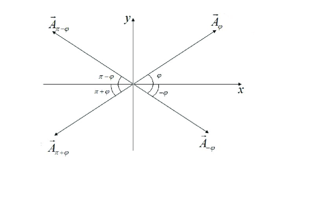
Figure 2: Four vectors that are transformed by the elements of quadruple group $V$.

The orientation of vector $A_{\pi-\varphi}$, presented in Fig.2, is obtained from $A_{\varphi}$ by means of mirror reflection relative to the plane passing through the axis $0y$ perpendicular to the figure plane $\sigma_{y}$. The orientation of vector $A_{\pi+\varphi}$ is obtained by means of rotation by angle $\pi$ about an axis, passing perpendicular to the figure through the origin of the coordinate system $C_{2}$ (axis of rotation of the second order). The symmetry elements $\sigma_{x},~{}\sigma_{y}$ and together with the unit element form quadruple group $V:~{}e,~{}\sigma_{x},~{}\sigma_{y},~{}C_{2}$. Now it is possible to bring the elements of two group to one-to-one correspondence: $G(-\varphi)\rightarrow\sigma_{x},~{}G(\pi-\varphi)\rightarrow\sigma_{y},~{}G(\pi+\varphi)\rightarrow C_{2},~{}e\rightarrow e$ that proves the isomorphism of above mentioned groups.

Each of three elements $a,~{}b,~{}c$ in combination with unit $e$ forms a subgroup

$$G~{}~{}~{}~{}~{}\begin{array}[]{ccc}\supset G_{+}&:e,&b,\\ \supset G_{-}&:e,&c,\\ \supset G_{0}&:e,&a.\\ \end{array}$$ (18)

Each of subgroups $G_{0},~{}G_{+},~{}G_{-}$ is the invariant subgroup in-group $G$. The presence of the three invariant subgroups of the second order indicates the existence of three factor-group (4:2=2) of the second order.

$$F_{0}:E(e,a),A(b,c),$$

$$F_{+}:E(e,b),A(a,c),$$

$$F_{-}:E(e,c),A(a,b).$$ (19)

Here we introduced notations, common for the group theory: $E$ stands for a unit element of factor-group; $A$ stands for an element of factor-group. Group $G$ is homomorphous to its factor-groups $F_{0}$ and $F_{\pm}$. As we see from (16) the elements of factor-group are formed as a result of unification of certain two elements of group $G$. This kind of unification of the elements of group $G$ indicates pair merging of energy levels $ce_{2m},~{}ce_{2m+1},~{}se_{2m+1}$ and $se_{2m+1}$. Therefore, three kinds of double degeneration, corresponding to the three factor-groups $F_{0}$ and $F_{\pm}$, appear in the energy spectrum. This happens owing to the presence of parameter $l$. Therefore, for the different values of parameter $l$ energy spectrum may be different at least qualitatively. Let us find out how to present combination of such a variety in energy spectrum

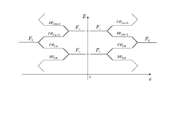
Figure 3: Fragment of energy spectrum of quantum pendulum, composed from theoretical-group consideration.

Factor-group $F_{0}$ is responsible for pair unity of levels of the same symmetry relative to the center of potential well $G(\pi-\varphi)$ (Fig.1). Quantum vibration motion appears because of this unification. In Fig.3. these levels are arranged to the extreme left and right from the ordinate axis.

Factor-groups $F_{0}$ and are responsible for pair unity of equations $ce_{n}$ and $se_{n}(n=1,2,\ldots)$ and for formation of clockwise and counter clockwise quantum rotation motion. In Fig.3 corresponding degenerated levels are found in both sides close to the ordinate axis. Numerical calculations Janke-Emde-Losh (see Fig.4), of Mathieu characteristics $a(l)$ and $b(l)$ prove that energy spectrum of quantum pendulum has a very complicated form and manifests all the main features of the spectrum presented in Fig.3.

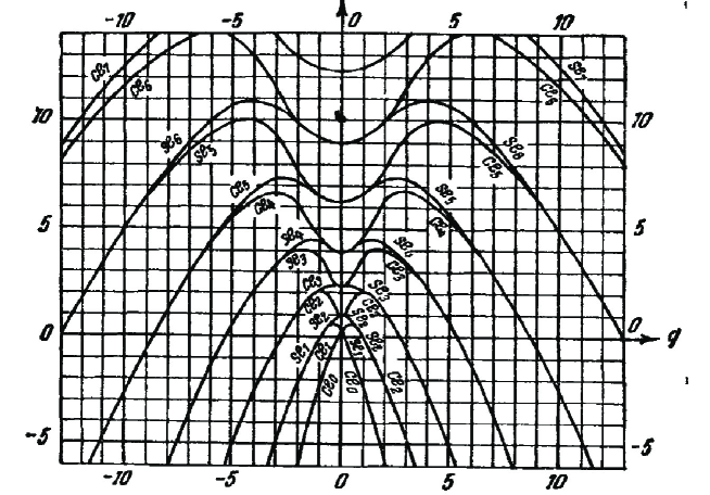
Figure 4: The group of the eigenvalues of $a_{n}(l)$ and $b_{N}(l)$ as functions of $l$ are plotted by numerical methods Bateman .

Similarity of the plots presented in Fig.3 and Fig.4 is obvious. Namely, both of them hold symmetry with respect to Y-axis. From both sides of Y-axis same eigenstates are coupled (degenerated). Only difference is that Fig.3 belongs to the theoretical group analysis, while Fig.4 is plotted using numerical methods. Both of these methods have their advantage and disadvantage. Only way to evaluate exact positions of branch points is to use numerical methods. From the other hand, eigenfunctions for each domain should be defined using theoretical algebraic methods. For more details see Chotorlishvili .

I.4 The Physical Problems are Reduced to Quantum Pendulum

We have already met with one physical problem that can get reduced to the solution of a quantum pendulum (9) - this is problem of quantum nonlinear resonance. Now we will get to know with other quantum-mechanical problems, that also get reduced to the solution of quantum pendulum.

As is known Herzberg ; Flygare , one of the forms of internal motion in polyatomic molecules is torsion oscillation which for sufficiently large amplitudes transforms to rotational motion. In order to describe the corresponding motion in Hamiltonian we assume that $\varphi$ is the angle of torsion of one part of the molecule with respect to the other part and replace the mass $m$ by the reduced moment of inertia $I=I_{1}I_{2}/(I_{1}+I_{2})$, where $I_{1}$ and $I_{2}$ are the inertia moments of rotation of the parts of the molecule with respect to its symmetry axis. Thus we obtain Gvarjaladze

$$U(\varphi)=\frac{V_{0}}{2}(1-\cos n\varphi)$$ (20)

where $V_{0}$ defines the height of potential barrier that separates torsion oscillations from the rotation of one part of the molecule with respect to the other part, and n defines the quantity of equilibrium orientations of one part of the molecule with respect to the other part. For the molecule of ethane $H_{3}C-CH_{3}$ , dimethylacetylene $H_{3}C-C\equiv C-CH_{3}$ and for other organic molecules we have $n=3$ equilibrium configurations (see Fig.5.).

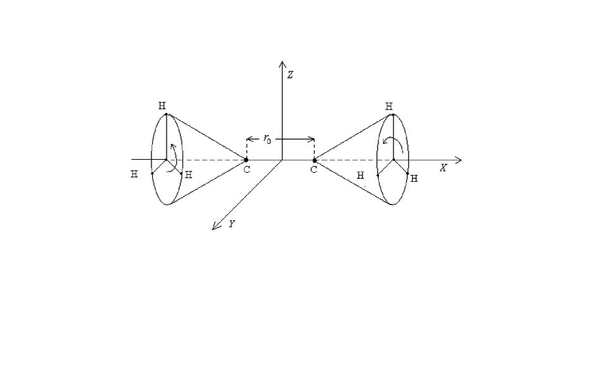
Figure 5: A schematic drawing of the molecular structure of ethane $H_{3}C-CH_{3}$. The circular arrow shows the torsion phase $\varphi,~{}r_{0}$ is the equilibrium distance between two parts of molecule.

The configuration shown in Fig.5 corresponds to an energy maximum and is a non-equilibrium configuration (cis-configuration). Other non-equilibrium configurations are obtained by rotating by the angles $\frac{2\pi}{3}$ and $2\frac{2\pi}{3}.$ Equilibrium configurations (trans-configurations) are obtained by rotating of the angles $\frac{\pi}{3},~{}\frac{\pi}{3}+\frac{2\pi}{3},~{}\frac{\pi}{3}+2\frac{2\pi}{3}$.

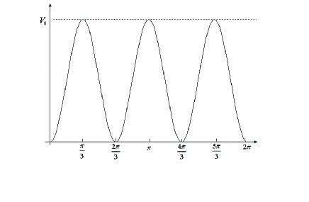
Figure 6: Potential energy curve of torsion motions in $H_{3}C-CH_{3}$. Phase $\varphi=0$ corresponds to equilibrium trance-configuration.

Below we give the numerical values Herzberg ; Flygare of other parameters of some organic molecules having the property of internal rotation. Thus for the molecule of ethane $C_{2}H_{6}$ we have $I_{1}=I_{2}\approx 5.3\cdot 10^{-47}kg\cdot m^{2}$, $V_{o}(C_{2}H_{6})\approx 2.1\cdot 10^{-20}J$, and for the molecule of dimethylacetylene $C_{4}H_{6}$ we have $I_{1}=I_{2}\approx 10.6\cdot 10^{-47}kg\cdot m^{2}$, $V_{o}(C_{4}H_{6})\approx 0.34\cdot 10^{-20}J$.

The Schrodinger equation corresponding to Hamiltonian (7) has the form

$$\frac{d^{2}\psi}{d\varphi^{2}}+\frac{2I}{\hbar^{2}}[\varepsilon_{k}-\frac{1}{2}V_{0}(1-\cos n\varphi)]\psi=0,$$ (21)

where $\varepsilon_{k}$ is the eigenenergy of the $k-th$ state. Note that $\varepsilon_{k}\equiv\varepsilon_{k}(V_{o})$ is the function of barrier height $V_{o}$. The condition of motion near the separatrix (near a potential maximum) is written in the form $\varepsilon_{k}\approx V_{o}$. If we introduce the new variable $\alpha=\frac{n\varphi}{2}$, then equation (18) can be rewritten as

$$\frac{d^{2}\psi(\alpha)}{d\alpha^{2}}+[E-2l_{0}\cos 2\alpha]\psi(\alpha)=0,$$ (22)

where

$$E=\frac{8I}{n^{2}\hbar^{2}}(\epsilon-V_{0}/2)$$ (23)

plays the role of energy in dimensionless units, and the parameter

$$l_{0}=\frac{2I}{n^{2}\hbar^{2}}V_{0}$$ (24)

is the half-height of the barrier in dimensionless units and plays the same role as the length of the thread does in the classical pendulum problem.

As our next example, we consider the vibration dynamics of a triatomic floppy molecule: the $LiNC/LiCN$ isomerizing system which has been extensively studied Essers ; Arranz . This molecule presents two stable isomers corresponding to the linear configurations, $Li-NC$ and $Li-CN$, which are separated by a relatively modest energy barrier. The motion in the beginning is very floppy, and then the Li atom can easily rotate around the $CN$ fragment

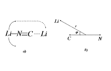
Figure 7: a) The relative motion of atom $Li$ to hard fragment $C\equiv N$. b) Coordinates $r$ and $\varphi$ describe relative motion $Li$ to fragment $C\equiv N$.

One can describe relative motion of $Li$ to hard fragment $C\equiv N$ by means of two coordinates: $\varphi$ - angle of orientation of $Li$ with respect to hard fragments axis and $r$ distance between atom $Li$ and mass center of fragment $C\equiv N$. Angle $\varphi=0$ corresponds to $Li-CN$ and $\varphi=\pi$ corresponds to its isomer $CNLi$. It is easy to make sure, that such isomerization process may be described by using the potential (17), when $n=2$. We obtain Schrodinger equation for such case in the same form, as we had for previous one (19).

I.5 Degenerate states of Mathieu-Schrodinger equation.

In the theory of Mathieu functions, the graphs of the eigenvalues $a_{n}(l)$ and $b_{n}(l)$ as functions of $l$ are plotted by numerical methods Bateman . As seen from these graphs, curves $a_{n}(l)$ and $b_{n}(l)$ merge for small $l$, while curves $a_{n}(l)$ and $b_{n+1}(l)$ merge for large $l$. It is obvious that the merged segments of the Mathieu characteristics correspond to the degenerate states whose existence has been mentioned above. In this section, we will define the wave functions of degenerate states. Below, the presence of branch points will play an essential role in explaining the transition from the pure state to the mixed one during the quantum investigation of the dynamics near the classical separatrix. In what follows, we will use the plane with coordinates $l$, $E$. In the classical consideration, the motion of a mathematical pendulum in a neighborhood of the separatrix occurs when the initial kinetic energy of the pendulum is close to the maximal potential one. It is obvious that, on the plane $(l,E)$, to this condition there corresponds the straight line $E=2l$. Therefore we can say that, on the plane $(l,E)$, to non-degenerate states there corresponds a certain domain lying on both sides of the line $E=2l$. It is in this very domain of the change of $l$ that the system is characterized by symmetry group $G$.

$$a)~{}Degeneration~{}of~{}states~{}at~{}small~{}l~{}(area~{}from~{}the~{}left~{}of~{}the~{}separatrix~{}line)$$

In the limit $l\rightarrow 0$ the equation of the Mathieu - Schrodinger (9) takes the form:

$$\frac{d^{2}\psi_{n}}{d\varphi^{2}}+E_{n}\psi_{n}=0$$ (25)

The orthonormal system of solutions of the equation (22) consists of even and odd solutions

$$\psi_{g}=\cos n\varphi,~{}\psi_{u}=\sin n\varphi.$$ (26)

They both correspond to the same energy value $E_{n}=n^{2}$. Note that functions (23) correspond also to the well-known asymptotic $(l\rightarrow 0)$ forms of the Mathieu functions [9]:

$$ce_{n}(\varphi)\rightarrow\cos n\varphi),~{}se_{n}(\varphi)\rightarrow\sin n\varphi.$$ (27)

This means that at the diminution of $l$ the coming together of the energy terms with the identical $n$ takes place and for $l=0$ they are merged together. It is necessary to find out that this confluence happens at the point $l=0$ or at $l=l^{(n)}_{-}\neq 0$. In this section, below we will be concerned with finding a lower point of the merging of terms $l^{(n)}_{-}$. At first let us find out what the eigenfunctions of the degenerated states corresponding to the level $E_{n}=n^{2}$ look like. Equation (22) is the Schrodinger equation for free rotation in the phase plane $\varphi$. The continuous Abelian group of two-dimensional rotations $O^{+}(2)$ Hamermesh corresponds to this motion.

Since the Abelian group may have only one-dimensional irreducible representations, the two-dimensional representation constructed in the base of real-valued functions (23) will be reducible. Hence functions (23) cannot be eigenfunctions of a degenerate state. To surmount this problem we shall recollect that the eigenfunctions for the degenerate condition can be also complex.

As is known Landau , symmetry relative to the change of time sign in the Schrodinger equation, accounts for the fact that the complex-conjugate wave functions correspond to one and the same energy eigenvalue. Therefore two complex-conjugate representations $\psi_{n}(\varphi)$ and $\psi^{\ast}_{n}(\varphi)$ should be regarded as a representation of doubled dimension. Usually, for the basis of the irreducible representation of the group $O^{+}(2)$ complex functions are assumed Hamermesh ,

$$\psi_{n}(\varphi)=e^{-in\varphi}.$$ (28)

Therefore, in the degenerate domain, in view of conditions of normalization, following complex conjugate functions should be considered as eigenfunctions

$$\psi_{n}(\varphi)=\frac{\sqrt{2}}{2}e^{-in\varphi},~{}\psi^{\ast}_{n}(\varphi)=\frac{\sqrt{2}}{2}e^{in\varphi}.$$ (29)

Let us remark that group $O^{+}(2)$ is isomorphic to subgroup $G_{-}$ (24). The element of the symmetry $c=G(\varphi\rightarrow\pi+\varphi)$ of the subgroup $G_{-}$ provides recurrence of the phase variation after each period and consequently the symmetry $G_{-}$ characterizes the condition of motion similar to the classical rotary motion. However, to use only the argument of symmetry is not sufficient for finding the coordinates of the branching point $l^{(n)}_{-}$. Below to find these points we use the secular perturbation theory. So, at $l=0$ we have doubly degenerate states with the wave functions (26). Let us find out, whether the perturbation

$$V(l,\varphi)=l\cos 2\varphi,~{}~{}l\ll 1$$ (30)

can remove the existing degeneration. It is known that, first order terms of the perturbation theory for the energy eigenvalues and the exact functions of zero approximation for double degenerate levels look like Landau

$$E^{(1)}_{0\pm}=\frac{1}{2}[(V_{11}+V_{22})\pm\sqrt{(V_{11}+V_{22})^{2}+4\cdot|V_{12}|^{2}}],$$

$$\psi_{n}^{\pm}=\psi^{(0)}=C_{1}\cdot\psi_{1}^{0}+C_{2}\cdot\psi_{2}^{0},$$

$$C_{1}^{(0)}=\bigg{\{}\frac{V_{12}}{2|V_{12}|}\bigg{[}1\pm\frac{V_{11}-V_{22}}{\sqrt{(V_{11}+V_{22})^{2}+4\cdot|V_{12}|^{2}}}\bigg{]}\bigg{\}}^{1/2}$$

$$C_{2}^{(0)}=\pm\bigg{\{}\frac{V_{21}}{2|V_{12}|}\bigg{[}1\mp\frac{V_{11}-V_{22}}{\sqrt{(V_{11}+V_{22})^{2}+4\cdot|V_{12}|^{2}}}\bigg{]}\bigg{\}}^{1/2}$$ (31)

where the index in brackets corresponds to the order of the perturbation theory, matrix elements of the perturbation (27) $V_{ik}(i,k=1,2)$ are calculated by using of functions (26) of the degenerate state of the non-perturbed Hamiltonian. Taking into account expressions (26) we shall calculate the matrix elements:

$$V_{11}=l\int_{0}^{\pi}\psi_{n}^{\ast}(\varphi)\cdot\psi_{n}(\varphi)\cos 2\varphi d\varphi=0,~{}V_{22}=0,$$

$$V_{12}=l\int\limits_{0}^{\pi}\Psi_{0}^{2}(\varphi)\cdot\cos 2\varphi d\varphi=\left\{\begin{array}[]{ll}0&\textrm{if $n\neq 1$}\\ \frac{l\pi}{4}&\textrm{if $n=1$}\end{array}\right.$$

After substitution of those matrix elements in the expressions (28) for the eigenvalues and exact eigenfunctions we shall obtain:

$$E_{\pm}^{(1)}=\pm\frac{l\pi}{4},~{}~{}\psi_{n=1}^{+}=\cos\varphi,~{}~{}\psi_{n=1}^{-}=-i\sin\varphi.$$ (32)

Thus, the exact wave functions (29) of the non-degenerate state only for $n=1$ coincide with the Mathieu function in the limit $l\rightarrow 0$ (24).

The perturbation $V(l,\varphi)$ removes degeneration only for the state n=1. Therefore it is only for the state $n=1$ that the spectrum branching occurs at the point $l=0$, which agrees with numerical calculations given in the form of diagrams (see Fig. 4.). It can be assumed that in the case of diminishing $l$, the merging of energy terms for states $n\neq 1$ takes place at the point at which the states are still defined by the Mathieu functions and not by their limiting values (24). Wave functions for degenerate states $l\neq 0,~{}n\neq 1$ can be composed from the Mathieu functions by using the same arguments as have been used above in composing the wave functions for $l\rightarrow 0)$. As a result, we obtain

$$\psi_{+}^{2m+1}=\psi_{n}(l,\varphi)=\frac{\sqrt{2}}{2}(ce_{n}\varphi\pm ise_{n}\varphi),~{}n=2m+1,$$

$$\psi_{-}^{2m+2}=\psi_{n}^{\ast}(l,\varphi)=\frac{\sqrt{2}}{2}(ce_{n}\varphi\pm ise_{n}\varphi),~{}n\neq 1,~{}l\neq 0,~{}n=2m+2.$$ (33)

Let us assume that at $l_{n}=l^{(n)}_{-}$ the removal of degeneration for the $n-th$ energy term happens.

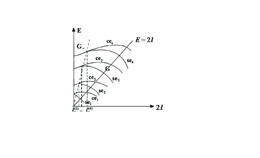
Figure 8: The energy levels as function of parameter $l$ on the plane $(E,l)$ on the left area from the separatrix line. The points of the branching of curves represent the boundaries between degenerate and non-degenerate states.

$$b)~{}Degenerate~{}state~{}at~{}major~{}l.~{}The~{}area~{}on~{}the~{}right~{}of~{}the~{}separatrix~{}line.$$

With the increasing of $l$ the particle can be trapped in a deep potential well ($V=l\cos 2\varphi,~{}0<\varphi<\pi$ Fig. 1.), and perform oscillatory motion. Properties of wave functions of quantum oscillator near to the bottom of the well are well known. This is the alternation of even and odd wave functions relative to the center of the potential well $\pi/2$ and presence of zeros in wave functions. With the help of the third column of Table 1 it is possible to write symmetry conditions close to $\pi/2$:

$$ce_{m}(\frac{\pi}{2}+\varphi)=(-1)^{m}ce_{m}(\frac{\pi}{2}-\varphi)$$

$$se_{m}(\frac{\pi}{2}+\varphi)=(-1)^{m+1}se_{m}(\frac{\pi}{2}-\varphi)$$ (34)

i.e. $ce_{2m}(\varphi),~{}se_{2m+1}(\varphi)$ are even functions and $se_{2m}(\varphi),~{}ce_{2m+1}(\varphi)$ are odd functions. Functions $ce_{2m}(\varphi),~{}se_{2m+1}(\varphi),~{}ce_{2m+1}(\varphi)$ and $se_{2m+1}(\varphi)$ have $m$ real zeros between $\varphi=0$ and $\varphi=\pi/2$ (not considering zeros on edges). The existing alternation of states (Fig. 8.) in area along the line of the separatrix is conditioned by the properties of states at the small $l$. With the help of the expressions (31) it is possible to determine easily, that in the spectrum of the states along the line $E=2l$ two (instead of one) even states alternate with odd states and so on. To get the alternation, caused now by properties at major $l$, two even conditions must degenerate in one even and two odd - in one odd. So we come to the conclusion, that two levels with wave functions $ce_{2m}(\varphi)$ and $se_{2m+1}(\varphi)$ coming nearer amalgamate in one level, and the following two levels $ce_{2m}(\varphi)$ and $se_{2m+1}(\varphi)$ also in one level. The levels obtained in this way will be doubly degenerated. It can be assumed that with the growth of $l$ the states defined by the symmetry group $G$ transform to the states with the symmetry of an invariant subgroup $G_{+}$ (15). This transformation takes place at the merging point of non-degenerate terms $l_{n}=l^{(n)}_{+}$. Recall that subgroup $G_{+}$ contains two elements: the unit element e and the reflection element with respect to the symmetry center of the well $b=G(\varphi\rightarrow\pi-\varphi)$. Complex wave functions of the area of degenerate states, with the symmetry of the invariant subgroup $G_{+}$, can be composed of pairs of functions of merged states in the same manner as we have done above for the area of small $l$ for states with the symmetry of $G_{-}$.

Not iterating these reasons, we shall write complex wave functions corresponding to the degenerated states in the form

$$\xi^{\pm}_{2n}(\varphi)=ce_{2n}(\varphi)\pm se_{2n+1}(\varphi)~{}~{}even~{}state$$

,

$$\xi^{\pm}_{2n+1}(\varphi)=ce_{2n+1}(\varphi)\pm se_{2n+2}(\varphi)~{}~{}odd~{}state$$ (35)

In the base of complex wave functions $\xi^{\pm}_{2n}$ and $\zeta^{\pm}_{2n+1}$ the indecomposable representation of the subgroup $G_{+}$ (15), is realized. Evenness of the wave functions $\xi$ and $\zeta$ with respect to the transformation $b=G(\varphi\rightarrow\pi-\varphi)$ of the subgroups $G_{+}$ characterizes an important property of wave functions evenness of the quantum oscillatory process. The results, obtained in this section, are plotted in Fig. 9.

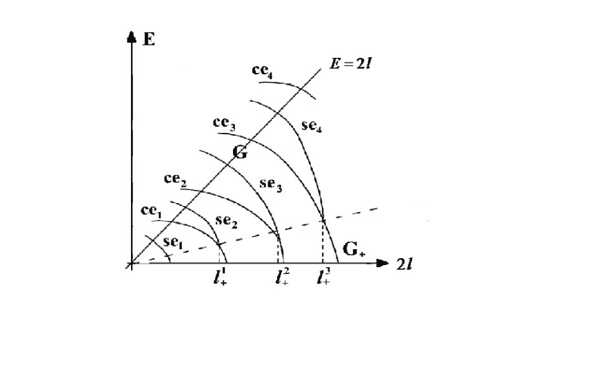
Figure 9: Energy levels as a function of the parameter $l$ on the plane $(E,l)$ to the area right from the separatrix line. The points of branching of curves represent degeneration points of terms in this area.

Figures 8 and 9 supplement each other: in the field of intersection with the separatrix the curves of the Figs. 8 and 9 are smoothly joined. So, we shall add up outcomes obtained in this section. The Mathieu-Schrodinger equation has an appointed symmetry. The transformations of the symmetry of the Mathieu functions form group $G$, which is isomorphic to the quaternary group of Klein. To this symmetry on a plane $(E,l)$ corresponds the appointed area along the line of the separatrix $E=2l$, containing non-degenerated energy terms. This area is restricted double sided by the areas of degenerate states, which are characterized by the symmetry properties of the invariant subgroups $G_{-}$ and $G_{+}$, respectively. The boundaries of these areas are defined by the branching points of energy terms existing both on the right and on the left of the separatrix.

The area of degenerate states is the quantum-mechanical analogs of two forms of motion of the classical mathematical pendulum-rotary and oscillatory. Comparing results of quantum reviews with classical, we remark that these two conditions of motion at quantum reviewing are divided by the area of a finite measure, whereas at the classical reviewing measure the separatrix is equal to zero.

I.6 Quantum analog of the stochastic layer.

In the case of Hamiltonian systems, performing a finite motion, a stochastic layer formed in a neighborhood of the separatrix under the action of an arbitrary periodic perturbation is a minimal phase space cell that contains the features of stochasticity Sagdeev . In this section we shall try to find out what can be considered as the quantum analog of the stochastic layer.

Let us assume that the pumping amplitude is modulated by the slow variable electromagnetic field. The influence of modulation is possible to take into account by means of such replacement in the Mathieu-Schrodinger equation (9),

$$l\rightarrow l_{0}+\Delta l\cos\nu t,~{}~{}\Delta l<l_{0}.$$ (36)

Here $\Delta l$ stands for the amplitude of modulation in dimensionless unit (see (10)), $\nu$ is the frequency of modulation. We suppose, that the slow variation of l can embrace some quantity of the branching points on the left and on the right of separatrix line (Figs. 8,9)

$$\Delta l\geq|l_{+}^{n}-l_{-}^{n}|,~{}~{}n=1,2,...N.$$ (37)

As a result of replacement (33) in the Hamiltonian (7), we get

$$\hat{H}=\hat{H}_{0}+\hat{H}^{\prime}(t),$$ (38)

$$\hat{H}^{\prime}(t)=\Delta l\cos 2\varphi\cos\nu t,$$ (39)

where $H_{0}$ is the universal Hamiltonian (7) and $\hat{H}^{\prime}(t)$ is the perturbation appearing as a consequence of pumping modulation.

It is easy to see, that the matrix elements of perturbation (36) $\hat{H}^{\prime}(t)$ for non-degenerate states equal zero. Really, having applied expansion formulas of the Mathieu functions in the Fourier series Janke-Emde-Losh it is possible to show

$$<ce_{n}|\hat{H}^{\prime}(t)|se_{n}>\sim\int_{0}^{2\pi}ce_{n}(\varphi)\cos 2\varphi se_{2n}(\varphi)d\varphi=0$$ (40)

simultaneously for the even and odd n. The expressions of the selection rules (37) will be fulfilled for values $l$ from the area $l^{n}_{-}\leq l\leq^{n}_{+}l$ Transitions between levels cannot be conditioned by time-dependent perturbation (36). It is expedient to include perturbation in the unperturbed part of the Hamiltonian. The Hamiltonian, obtained in such way, is slowly depending on the parameter $l$. So, instead of (35) and (36) for the non-degenerated area $G$ we get the Hamiltonian in the form

$$\hat{H}=-\frac{\partial^{2}}{\partial\varphi^{2}}+l(t)\cos 2\varphi,$$ (41)

$$l(t)=l_{0}+\Delta l\cos\nu t.$$ (42)

There arises the situation in which the system slowly ”creeps” along the Mathieu characteristics and, in doing so, encloses the branching points on the left $l^{n}_{-}$ or on the right $l^{n}_{+}$. a)  Irreversible  ”creeping”  of  energy  term  populations  due  to  the  influence  of  a  measuring  arrangement.

According to the general rules of quantum mechanics, probabilities that the system will pass to the eigenstate of another area are defined by the coefficients of expansion of the wave function of one area into the eigenfunctions of another area. Let us assume that, initially, the system was in one of the eigenstates from the non-degenerate area $G$, for example, in the state $ce_{2n}$. After a quarter of the modulation period $T/4$ (where $T=2p/n$), having passed through the point $l^{n}_{-}$, the system finds itself in the degenerated area $G_{-}$. In this case the system will pass to degenerate states $\psi^{\pm}_{2n}$ with probabilities,

$$P(ce_{2n}\rightarrow\psi_{2n}^{\pm})=|\frac{1}{\pi}\int_{0}^{2\pi}ce_{2n}(\varphi)\psi_{2n}^{\pm\ast}(\varphi)d\varphi|^{2}=$$

$$=\frac{1}{2\pi}|\int_{0}^{2\pi}ce_{2n}(\varphi)(ce_{2n}(\varphi)\pm ise_{2n}(\varphi))^{\ast}d\varphi|^{2}=1/2.$$ (43)

For deriving (40) we used the condition of normalization (12) and orthogonality [9]

$$\int_{0}^{2\pi}ce_{k}(\varphi)se_{l+1}(\varphi)d\varphi=0,~{}l,k=0,1,2,...).$$ (44)

The passage (40) is based on the assumption of having a deep physical sense. As is generally known, in quantum mechanics symmetry with respect to both directions of time is expressed in the invariance of the Schrodinger equation with respect to the variation of the sign of time $t$ and simultaneous replacement $\psi$ by way of $\psi^{\ast}$. However, it is necessary to remember that this symmetry concerns only the equations, but not the concept of a measurement playing a fundamental role in the quantum mechanics Landau ; Kaempffer . ”Measurement” is understood as the process of interaction of the quantum system with the classical object usually called ”instrument.” Under the measuring arrangement, consisting of the analyzer and detector, one must not imagine the laboratory’s instrument. In our case, the role of the instrument plays in our case the modulating field, which is capable to ”drag” the system through the branching points. When passing through the branching point from one area to another, the state remains unchanged. However, being an eigenstate in one area, it will not be an eigenstate in another. At the passage through branching points there occurs a spectral expansion of the initial wave function belonging to the region of one symmetry over the eigenfunctions belonging to the region of another symmetry. The presence only of the analyzer reserves a pure state and the process remains reversible. So, passage through the branching point plays role of analyzer. Further we shall assume the presence of the detector, defining which of the states $\psi_{n}^{+}$ or $\psi_{n}^{-}$ is involved in passage. The transition of the system to various states defined by probabilities (40) is fixed by means of the action of the detector. The presence of the detector is expressed formally in averaging with respect to phase and neglecting the interference term usually appearing in the expression for a distribution function. As a result of averaging the partial loss of information about the condition of the system takes place and a mixed state is generated. In our problem role of detector will play effect self-chaotization, which appeared in degenerate region (see next subsection).

As is follows from (40), after the quarter period degenerated rotary states $\psi_{2n}^{+}$ and $\psi_{2n}^{-}$ will be occupied with the identical probability. After the half period $\frac{1}{2}T$ the system again appears in the area $G$ going through the branching point $l_{-}^{n}$ in the reverse direction. At the same time there appear probabilities, of the transition into the states $ce_{n},~{}se_{n}$, and both of them are distinct from zero

$$P(\psi_{2n}^{\pm}\rightarrow ce_{2n})=\frac{1}{2}|\frac{1}{\pi}\int_{0}^{2\pi}(ce_{2n}(\varphi)\pm ise_{2n}(\varphi))ce_{2n}(\varphi)d\varphi|^{2}=\frac{1}{2},$$ (45)

$$P(\psi_{2n}^{\pm}\rightarrow se_{2n})=\frac{1}{2}|\frac{1}{\pi}\int_{0}^{2\pi}(ce_{2n}(\varphi)\pm ise_{2n}(\varphi))se_{2n}(\varphi)d\varphi|^{2}=\frac{1}{2}.$$ (46)

Here we have used again normalization (12) and orthogonality relations (41). It is easy to write transition probability from $ce_{2n}$ into one of the degenerated states $\psi_{2n}^{\pm}$ and back in the $ce_{2n}$

$$P(ce_{2n}\leftrightarrow ce_{2n})\equiv P(ce_{2n}\rightarrow\psi_{2n}^{\pm}\rightarrow ce_{2n})=$$

$$=P(ce_{2n}\rightarrow\psi_{2n}^{+})P(\psi_{2n}^{+}\rightarrow ce_{2n})+P(ce_{2n}\rightarrow\psi_{2n}^{-})P(\psi_{2n}^{-}\rightarrow ce_{2n}).$$ (47)

Here the first summand corresponds to the passage through the degenerated state $\psi_{2n}^{+}$ and the second one to the passage through $\psi_{2n}^{-}$. It is easy to see with the help of previous computations (40), (42), and (43) that contributions of these passages are identical and individually equal to $1/4$. Therefore finally we have

$$P_{-}(ce_{2n}\leftrightarrow ce_{2n})=\frac{1}{2}.$$ (48)

Similarly it may be shown that transition probability from the state $ce_{2n}$ in one of the degenerated states $\psi_{2n}^{\pm}$ and back in the area $G$, in the state $se_{2n}$ by means of going through the point $l_{-}^{n}$ is

$$P(ce_{2n}\leftrightarrow se_{2n})=P(ce_{2n}\rightarrow\psi_{2n}^{+})P(\psi_{2n}^{+}\rightarrow se_{2n})+$$

$$+P(ce_{2n}\rightarrow\psi_{2n}^{-})P(\psi_{2n}^{-}\rightarrow se_{2n})=\frac{1}{2}\cdot\frac{1}{2}+\frac{1}{2}\cdot\frac{1}{2}=1/2.$$ (49)

Thus, the system being at the initial moment in the eigenstate $ce_{2n}$, at the end of half-period of modulation appears in the mixed state $\rho_{2n}$ in which the states $ce_{2n}$ and $se_{2n}$ are intermixed with identical weight, and corresponding levels are populated with identical probabilities. After the expiration of quarter of cycle the system will pass from the area $G$ (the state $\rho_{2n}$) in the area $G_{+}$, going through the point $l_{n}^{+}$. In passages from the area $G_{+}$ four states take part $\xi_{2n}^{\pm}=\frac{1}{\sqrt{2}}(ce_{2n}\pm ise_{2n+1})$ and $\zeta_{2n-1}^{\pm}=\frac{1}{\sqrt{2}}(ce_{2n-1}\pm ise_{2n})$. So, with taking into consideration the above mentioned for the probabilities of transitions we get

$$P(\rho_{2n}\rightarrow\xi_{2n}^{\pm})=\frac{1}{4\pi}|\int_{0}^{2\pi}(ce_{2n}(\varphi)+se_{2n}(\varphi))(ce_{2n}(\varphi)\mp ise_{2n+1}(\varphi))d\varphi|^{2}=\frac{1}{4},$$ (50)

$$P(\rho_{2n}\rightarrow\zeta_{2n}^{\pm})=\frac{1}{4\pi}|\int_{0}^{2\pi}(ce_{2n}(\varphi)+se_{2n}(\varphi))(ce_{2n-1}(\varphi)\mp ise_{2n}(\varphi))d\varphi|^{2}=\frac{1}{4},$$ (51)

For deriving the last expressions in addition to the normalization conditions we have used the orthogonality conditions

$$\int_{0}^{2\pi}ce_{n}(\varphi)ce_{m}(\varphi)d\varphi=\int_{0}^{2\pi}se_{n+1}(\varphi)se_{m+1}(\varphi)d\varphi=0,~{}m\neq n.$$ (52)

On the basis of (47) and (48) we conclude, that after the time $\frac{3}{4}T$, system will be in the area $G_{+}$ in one of four oscillatory states $\xi_{2n-1}^{\pm}$ and $\zeta_{2n-1}^{\pm}$ with the identical probability equal to $1/4$.

After one cycle $T$ the system gets back in the area $G$, from which it started transition from the level $ce_{2n}$. Upon returning, four levels $ce_{2n},~{}se_{2n},~{}ce_{2n-1}$ and $se_{2n+1}$ will be involved. Calculating probabilities of passages from the oscillatory state of the area $G_{+}$, to these four levels we shall obtain

$$P(\xi_{2n}^{\pm}\rightarrow ce_{2n})=P(\xi_{2n}^{\pm}\rightarrow se_{2n+1}=1/2,$$ (53)

$$P(\xi_{2n-1}^{\pm}\rightarrow se_{2n})=P(\zeta_{2n-1}^{\pm}\rightarrow se_{2n-1}=1/2.$$ (54)

The probability of passages from the nondegenerated area to the area $G_{+}$ in one of the oscillatory states $\xi_{2n}^{\pm},~{}\zeta_{2n-1}^{\pm}$ and back in the area $G$ will be:

$$P_{+}(\rho_{2n}\leftrightarrow se_{2n})=P(\rho_{2n}\rightarrow\xi_{2n}^{\pm})P(\xi_{2n}^{+}\rightarrow se_{2n+1})+$$

$$+P(\rho_{2n}\rightarrow\xi_{2n}^{-})P(\xi_{2n}^{-}\rightarrow se_{2n+1})=\frac{1}{4}\cdot\frac{1}{2}+\frac{1}{4}\cdot\frac{1}{2}=\frac{1}{4}.$$ (55)

Similarly it is possible to show

$$P(\rho_{2n}\leftrightarrow ce_{2n})=P(\rho_{2n}\rightarrow se_{2n})=P(\rho_{2n}\rightarrow ce_{2n-1})=1/4.$$ (56)

Thus, after the lapse of time $T$ four levels of the nondegenerate area $G$ will be occupied with the identical probabilities $1/4$ (Fig. 10.) The motion of the system upwards on energy terms will cease upon reaching the level for which the points of the branching in Fig. 10 are on the distance at which the condition (34) no longer is valid. The motion of the system downwards will be stopped upon reaching the zero level. If the system at the initial moment is in the state $2n=N/2$, then after $N/2$ cycles of modulation all $N$ levels will be occupied. It is easy to calculate a level population for the extremely upper and extremely lower levels. Really, the level population for extreme levels is possible to define with the help of a Markov chain containing only one possible trajectory in the spectrum of Mathieu characteristics:

$$P(ce_{N/2},t_{0};ce_{N/2+1},t_{0}+\frac{T}{2},\dots ce_{N},t_{0}+N\frac{T}{2})=$$

$$P(se_{N},t_{0}+N\frac{T}{2}\leftarrow ce_{N-1},t_{0}+(N-1)\frac{T}{2})...$$

$$P(ce_{N/2+1},t_{0}+T\leftarrow se_{N/2+1},t_{0}+\frac{T}{2})P((se_{N/2+1},t_{0}+\frac{T}{2}\leftarrow ce_{N/2+1},t_{0}),$$ (57)

where $t_{0}$ is an initial time. Here, when discussing the transition probabilities from one state to another, we also use a time argument. It is possible to write a similar chain of level population for the extremely lower level. As the probabilities of passages, included in the right side of (54) by way of factors, are equal to $1/2$, then probabilities of an extreme level population will be $(1/2)^{N/2}$. As to the Markovian chain for non-extreme levels, it has a cumbersome form and we do not give it here.

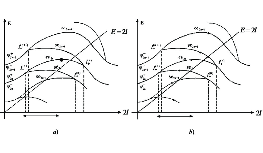
Figure 10: The fragment of the energy terms, participating in passages calculated in the text. a) The initial state. The particle is in the state of $ce_{2n}$. b) The final state. Levels which are affected by a change of the field amplitude get populated.

$$b)~{}Selfchaotization~{}produced~{}by~{}a~{}big~{}phase~{}"incursion"~{}of~{}the~{}probability~{}amplitude.$$

Different from the area of non-degenerate states $G$, in the areas of degenerate states $G_{-}$ and $G_{+}$, the non-diagonal matrix elements of perturbation $\hat{H}^{\prime}(t)$ (36) are not zero.

$$H^{\prime}_{+-}=H^{\prime}_{-+}=<\psi^{+}_{2n+1}|\hat{H^{\prime}(t)}|\psi^{-}_{2n+1}>\sim\Delta l\int\limits_{o}^{2\pi}\psi^{+}_{2n+1}\psi^{-\ast}_{2n+1}\cos 2\varphi d\varphi\not=0.$$ (58)

where the wave functions $\psi_{\pm}$ have been defined previously by (30). Here, for the brevity of the notation, we omit the upper indices indicating the quantum state. An explicit dependence of $\hat{H}^{\prime}(t)$ on time given by the multiplier $\cos\nu t$ is assumed to be slower as compared with the period of passages from one degenerate state to another produced by the non-diagonal matrix elements $H^{\prime}_{+-}$. Therefore below, perturbations $\hat{H}^{\prime}(t)$ will be treated as time-independent perturbations able to produce the above-mentioned passages. Therefore in the area of degenerate states the system can be found in the time-dependent superposition state Landau ; Bohm :

$$\psi_{2n}(t)=C^{+}_{n}(t)\psi^{+}_{2n}+C^{-}_{n}(t)\psi^{-}_{2n}.$$ (59)

Probability amplitudes $C^{\pm}_{n}(t)$ are found by means of the following fundamental quantum-mechanical equation expressing the causality principle:

$$-i\hbar\frac{dC^{+}_{n}}{dt}=(E_{on}+H^{\prime}_{++})C^{+}_{n}+H^{\prime}_{+-}C^{-}_{n},$$

$$-i\hbar\frac{dC^{-}_{n}}{dt}=H^{\prime}_{+-}C^{+}_{n}+(E_{on}+H^{\prime}_{--})C^{-}_{n}.$$ (60)

It is easy show that in the case of our problem it should be assumed that $H^{\prime}_{++}=H^{\prime}_{--}$ and $H^{\prime}_{+-}=H^{\prime}_{-+}$. Let us investigate changes that occurred in the state of the system during time $\Delta T$ while the system was in the area $G_{-}$, (i.e., during the time of movement to the left from $l_{-}^{n}$ and, reversal, to the right to $l_{-}^{n}$). It will be assumed that $T$ is part of the period of modulation $T$. For arbitrary initial values the system of equations (57) has a solution

$$C^{+}_{n}(t)=\frac{C_{+}(0)+C_{-}(0)}{2}exp[\frac{-i}{\hbar}(E-H^{\prime})t]+\frac{C_{+}(0)-C_{-}(0)}{2}exp[\frac{i}{\hbar}(E-H^{\prime})t],$$

$$C^{-}_{n}(t)=\frac{C_{+}(0)+C_{-}(0)}{2}exp[\frac{-i}{\hbar}(E-H^{\prime})t]-\frac{C_{+}(0)-C_{-}(0)}{2}exp[\frac{i}{\hbar}(E-H^{\prime})t],$$ (61)

where $E\rightarrow E_{0}+H^{\prime}_{++},~{}E\rightarrow E_{0}+H^{\prime}_{--},~{}H^{\prime}_{+-}\rightarrow H^{\prime}.$

After complementing $\hat{H}^{\prime}(t)$ (58) with the factor $\cos\nu t$, we can take into consideration also a slow time dependent change of perturbation $(H^{\prime}\rightarrow H^{\prime}\cos\nu t).$

Let motion begin from the state $\psi^{-}_{2n}$ of the degenerate area. Then as the initial conditions we take

$$C^{-}_{n}(0)=1,~{}C^{+}_{n}(0)=0$$ (62)

as initial conditions. Substituting (59) into (58), for the amplitudes $C_{\pm}(t)$ we obtain

$$C_{-}(t)=e^{(i/\hbar)Et}\cos\omega t,$$

$$C_{+}(t)=-ie^{(i/\hbar)Et}\sin\omega t,~{}\omega=\frac{H^{\prime}}{\hbar}.$$ (63)

Now, using (60), for the distribution $|\psi(t)|^{2}$ (56) we obtain

$$|\psi(t)|^{2}=\cos^{2}(\frac{H^{\prime}}{\hbar}t)|\psi_{-}(t)|^{2}+\sin^{2}(\frac{H^{\prime}}{\hbar}t)|\psi_{+}(t)|^{2}-$$

$$-\frac{1}{2}\sin(2\frac{H^{\prime}}{\hbar}t)[\psi_{+}(t)\psi^{\ast}_{-}(t)-\psi_{-}(t)\psi^{\ast}_{+}(t)].$$ (64)

In the expression for $|\psi(t)|^{2}$ the first two terms correspond to the transition probabilities $-\rightarrow+$ and $-\rightarrow+$, respectively, while the third term corresponds to the interference of these states. Distribution (61) corresponds to a pure state.

Note that (like any other parameter of the problem) the value $H^{\prime}$ contains a certain small error $\delta H^{\prime}\ll H^{\prime}$, which during the time of one passage $2\pi\hbar/H^{\prime}$ leads to an insignificant correction of the phase $2\pi(\delta H^{\prime}/H^{\prime})$. However, during the time $T$ a phase incursion takes place and a small error $\delta H^{\prime}$ may lead to uncertainty of phase $\sim(\delta H^{\prime}/\hbar)\Delta T$, which may turn out to be of order $2\pi$. In that case the phase becomes random. Therefore by the moment $\Delta T$ the distribution takes the form that can be obtained from (61) by means of averaging with respect to the random phase $\alpha=(\delta H^{\prime}/\hbar)\Delta T$.

Hence, after averaging expression (61), equating the interference term to zero and taking into account that

$$\overline{\sin^{2}[(H^{\prime}/\hbar)t]}=\overline{\cos^{2}[(H^{\prime}/\hbar)t]}=1/2$$

we get

$$|\psi|^{2}=\bar{|\psi(t)|^{2}}=\frac{1}{2}(|\psi_{+}|^{2}+|\psi_{-}|^{2}),$$ (65)

where the stroke above denotes the averaging with respect to time. The obtained formula (62) is the distribution of a mixed state, which contains probabilities of degenerate states $|\psi_{\pm}|^{2}$ with the same weights $1/2$. The assumption that a large phase is a random value that, after averaging, makes the interference term equal to zero is frequently used in analogous situations Bohm .

Thus we conclude that if the system remains in the areas $G_{\pm}$ of degenerate states for a long time, $\Delta T\gg 2\pi\hbar/H^{\prime},~{}\Delta T\approx 2\pi\hbar/\delta H^{\prime}$ during which the system manages to perform a great number of passages, then in the case of a passage to the nondegenerate area $G$ the choice of continuation of the path becomes ambiguous. In other words, having reached the branch point, the system may with the same probability continue the path along two possible branches of the Mathieu characteristics. The error $H^{\prime}$ is evidently connected with the error of the modulation amplitude value. It obviously follows that, when passing the branch point, the mixed state (62) will transform with a $1/2$ probability to the states $ce$ and $se$, as shown in formulas (42) and (43). Analogously, we can prove the validity of all subsequent formulas for the passage probabilities (44),(45).

$$c)~{}Kinetic~{}stage~{}of~{}evolution$$

We have already met with one physical problem that can get reduced to the solution of a quantum pendulum (9) - this is a problem of quantum nonlinear resonance. Now we will get to know with other quantum-mechanical problems, that also get reduced to the solution of quantum pendulum.

Note that the parameter $\omega$, which is connected with the modulation depth $\Delta l$, has (like any other parameter) a certain small error $\delta\omega$, which during the time of one passage $t\sim 2\pi/\omega$, leads to an insignificant correction in the phase $2\pi(\delta\omega/\omega)$. But during the time $t\sim\Delta T$, there occur a great number of oscillations ( phase incursion takes place) and, in the case $\Delta T\gg\tau$, a small error $\delta\omega$ brings to the uncertainty of the phase $\sim\Delta T\delta\omega$ which may have order $2\pi$. Then we say that the phase is self-chaotized.

Let us introduce the density matrix averaged over a small dispersion $\delta\omega$:

$$\rho^{+-}_{n}(t)=\left(\begin{array}[]{cc}W^{+}_{n}(t)&iF_{n}(t)\\ -iF^{\ast}_{n}(t)&W^{-}_{n}(t)\\ \end{array}\right),\,$$ (68)

where $W^{\pm}_{n}(t)=\overline{|C^{\pm}_{n}(t)|^{2}},~{}~{}F_{n}(t)=|\overline{C^{+}_{n}(t)C^{-\ast}_{n}(t)}|$. The overline denotes the averaging over a small dispersion $\delta\omega$

$$\overline{A(\omega,t)}=\frac{1}{2\delta\omega}\int\limits^{\omega+\delta\omega}_{\omega-\delta\omega}A(x,t)dx$$ (69)

To solve (64) we can write that

$$W^{+}_{n}(t)=\overline{\sin^{2}\omega t},~{}~{}W^{-}_{n}(t)=\overline{\cos^{2}\omega t},~{}~{}F_{n}(t)=\frac{1}{2}|\overline{\sin 2\omega t}|.$$ (70)

After a simple integration of the averaging (64), for the matrix element (65) we obtain

$$W^{\pm}_{n}(t)=\frac{1}{2}(1\mp f(2\delta\omega t)\cos 2\omega t),$$

$$F_{n}(t)=F^{\ast}_{n}(t)=\frac{1}{2}f(2\delta\omega t)\sin 2\omega t,$$ (71)

$$f(2\delta\omega t)=\frac{\sin 2\delta\omega t}{2\delta\omega t}.$$

At small values of time $t\ll\overline{\tau}~{}(\overline{\tau}=2\pi/\delta\omega)$, insufficient for self-chaotization $(f(2\delta\omega t)\approx 1)$, we obtain

$$W^{+}_{n}(t\ll\overline{\tau})=\sin^{2}\omega t,~{}~{}W^{-}_{n}(t\ll\overline{\tau})=\cos^{2}\omega t,~{}~{}F_{n}(t\ll\overline{\tau})=\frac{1}{2}\sin 2\omega t.$$

Comparing these values with the initial values (65) of the density matrix elements, we see that the averaging procedure (64), as expected, does not affect them. Thus, for small times we have

$$\rho^{+-}_{n}(t\ll\overline{\tau})=\left(\begin{array}[]{cc}\sin^{2}\omega t&\frac{i}{2}\sin 2\omega t\\ \frac{-i}{2}\sin 2\omega t&\cos^{2}\omega t\\ \end{array}\right).\,$$ (74)

One can easily verify that matrix (67) satisfies the condition $\rho(t\ll\overline{\tau})=\rho(t\ll\overline{\tau})$, which is a necessary and sufficient condition for the density matrix of the pure state.

For times even smaller than $t\ll\tau\ll\overline{\tau}$, when passages between degenerate states practically fail to occur, by taking the limit $\omega t\ll 1$ in (67), we obtain the following relation for the density matrix:

$$\rho^{+-}_{n}(t=0)=\rho^{+-}_{n}(t\ll\tau)=\left(\begin{array}[]{cc}0&0\\ 0&1\end{array}\right).\,$$ (75)

This relation corresponds to the initial condition (59) when the system is in the eigenstate $\psi^{-}_{2n}$. Let us now investigate the behavior of the system at times $t\geq\overline{\tau}$ when the system gets self-chaotized.

On relatively large time intervals $t\geq\overline{\tau}$, in which the self-chaotization of phases takes place, for the matrix elements we should use general expressions (66). The substitution of these expressions for the matrix elements (66) into the density matrix (63) gives

$$\rho^{+-}_{n}(t)=\frac{1}{2}\left(\begin{array}[]{cc}1-f(2\delta\omega t)\cos 2\omega t&if(2\delta\omega t)\sin 2\omega t\\ -if(2\delta\omega t)\sin 2\omega t&1+f(2\delta\omega t)\cos 2\omega t\\ \end{array}\right).\,$$ (78)

Hence, for times $t\geq\overline{\tau}$ during which the phases get completely chaotized, after passing to the limit $\delta\omega t\gg 1$ in (69), we obtain

$$\rho^{+-}_{n}(t\gg\overline{\tau})=\frac{1}{2}\left(\begin{array}[]{cc}1-O(\varepsilon)&iO(\varepsilon)\\ -iO(\varepsilon)&1+O(\varepsilon)\\ \end{array}\right),\,$$ (81)

where $O(\varepsilon)$ is an infinitesimal value of order $\epsilon=\frac{1}{2\delta\omega t}$.

The state described by the density matrix (70) is a mixture of two quantum states $\psi^{+}_{2n}$ and $\psi^{-}_{2n}$ with equal weights. The comparison of the corresponding matrix elements of matrices (70) and (69) shows that they differ in the terms that play the role of quickly changing fluctuations. When the limit is $t\gg\overline{\tau}$, fluctuations decrease as $\sim\frac{1}{2\delta\omega t}$ (see Fig. 11 and 12).

Thus the system, which at the time moment $t=0$ was in the pure state with the wave function $\psi^{-}_{2n}$ (68), gets self-chaotized with a lapse of time $t\gg\overline{\tau}$ and passes to the mixed state (70).

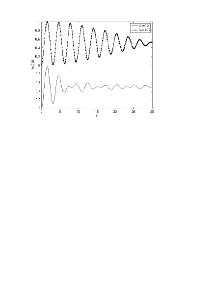
Figure 11: Time-dependence of the diagonal matrix element $W_{n}^{+}(t)$ of the density matrix (63), constructed by means of formulas (63), (66) for the parameter values $\omega=1/\tau=1,~{}C_{n}^{+}(0)=1,~{}C_{n}^{-}(0)=0.$ As clearly seen from the Figure, the higher the dispersion value of the parameter $\delta\omega$, the sooner the stationary value $W_{n}^{+}(t>\bar{\tau}\sim\frac{1}{\delta\omega})=\frac{1}{2}$ is achieved.

In other words, at the initial moment the system had a certain definite ”order” expressed in the form of the density matrix $\rho^{+-}_{n}(0)$ (68). With a lapse of time the system got self-chaotized and the fluctuation terms appeared in the density matrix (69). For large times $t\gg\overline{\tau}$ a new ”order” looking like a macroscopic order is formed, which is defined by matrix (70).

After a half-period the system passes to the area of nondegenerate states $G$ (68). In passing through the branch point, there arise nonzero probabilities for passages both to the state $ce_{2n}$ and to the state $se_{2n}$. Both states $\psi^{+}_{2n}$ and $\psi^{-}_{2n}$ will contribute to the probability that the system will pass to either of the states $ce_{2n}$ and $se_{2n}$. For the total probability of passage to the states $ce_{2n}$ and $se_{2n}$ we obtain respectively

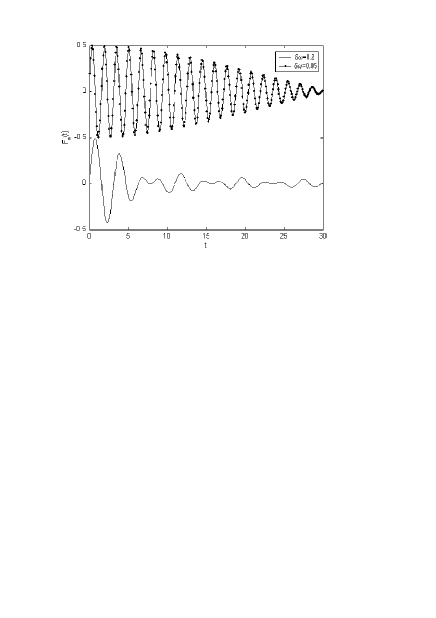
Figure 12: The vanishing of nondiagonal matrix elements of the density matrix (63) with a lapse of time $t>\bar{\tau}$ while the system remained in the degenerate area $G_{-}$. The graph is constructed for the parameter values $\omega=1/\tau=1,~{}C_{n}^{+}(0)=1,~{}C_{n}^{-}(0)=0.$, with the aid of formulas (63) and (66).

$$P(\rho^{+-}_{2n}(t\gg\tau)\rightarrow ce_{2n})=\frac{1}{2}\bigl{|}\frac{1}{\pi}\int\limits_{o}^{2\pi}\psi^{+}_{2n}(\varphi)ce_{2n}(\varphi)d\varphi\bigr{|}^{2}+$$

$$+\frac{1}{2}\bigl{|}\frac{1}{\pi}\int\limits_{o}^{2\pi}\psi^{-}_{2n}(\varphi)ce_{2n}(\varphi)d\varphi\bigr{|}^{2}=\frac{1}{2}\cdot\frac{1}{2}+\frac{1}{2}\cdot\frac{1}{2}=\frac{1}{2},$$

$$P(\rho^{+-}_{2n}(t\gg\tau)\rightarrow se_{2n})=\frac{1}{2}\bigl{|}\frac{1}{\pi}\int\limits_{o}^{2\pi}\psi^{+}_{2n}(\varphi)se_{2n}(\varphi)d\varphi\bigr{|}^{2}+$$

$$+\frac{1}{2}\bigl{|}\frac{1}{\pi}\int\limits_{o}^{2\pi}\psi^{-}_{2n}(\varphi)se_{2n}(\varphi)d\varphi\bigr{|}^{2}=\frac{1}{2}\cdot\frac{1}{2}+\frac{1}{2}\cdot\frac{1}{2}=\frac{1}{2}.$$ (82)

Thus, in the nondegenerate area the mixed state is formed, which is defined by the density matrix

$$\rho^{ik}_{2n}(t\sim\frac{T}{2}\gg\tau)=\frac{1}{2}\left(\begin{array}[]{cc}1&0\\ 0&1\\ \end{array}\right),\,$$ (85)

where $i$ and $k$ number two levels that correspond to the states $ce_{2n}$ and $se_{2n}$.

As follows from (72), at this evolution stage of the system, the populations of two nondegenerate levels get equalized. It should be noted that though the direct passage (37) between the nondegenerate levels is not prohibited, perturbation (36) essentially influences ”indirect” passages. Under ”indirect” passages we understand a sequence of events consisting a passage $G\rightarrow G_{-}$ through the branch point, a set of passages between degenerate states in the area $G_{-}$, and the reverse passage through the branch point $G_{-}\rightarrow G$. The ”indirect” passages ocurring during the modulation half period $T/2$ result in the equalization (saturation) of two nondegenerate levels.

As to the nondegenerate area, the role of perturbation $\hat{H}^{\prime}(t)$ in it reduces to the displacement of the system from the left branch point to the right one.

It is easy to verify that after states (72) pass to the states of the degenerate area $G_{+}$, we obtain the mixed state which involves four states $\xi^{\pm}_{2n}(\varphi)$ and $\zeta^{\pm}_{2n+1}(\varphi).$

Let us now calculate the probability of four passages from the mixed state $\rho^{ik}_{2n}$ (70) to the states $\xi^{\pm}_{2n}(\varphi)$ and $\zeta^{\pm}_{2n-1}(\varphi)$:

$$P(\rho^{ik}_{2n}\rightarrow\xi^{\pm}_{2n})=\frac{1}{2}\bigl{|}\frac{1}{\pi}\int\limits_{o}^{2\pi}(ce_{2n}(\varphi)+se_{2n}(\varphi))\xi^{\pm}_{2n}(\varphi)d\varphi\bigr{|}^{2}=\frac{1}{4},$$

$$P(\rho^{ik}_{2n}\rightarrow\zeta^{\pm}_{2n-1})=\frac{1}{2}\bigl{|}\frac{1}{\pi}\int\limits_{o}^{2\pi}(ce_{2n}(\varphi)+se_{2n}(\varphi))\zeta^{\pm}_{2n-1}(\varphi)d\varphi\bigr{|}^{2}=\frac{1}{4}.$$ (86)

As a result of these passages, in the area $G_{+}$ we obtain the mixed state described by the four-dimensional density matrix

$$\rho^{+-}_{2n,2n+1}(t\sim T\gg\tau)=\frac{1}{4}\left(\begin{array}[]{cccc}1&0&0&0\\ 0&1&0&0\\ 0&0&1&0\\ 0&0&0&1\\ \end{array}\right),\,$$ (91)

where the indices of the density matrix (26) show that the respective matrix elements are taken with respect to the wave functions $\xi^{\pm}_{2n}(\varphi)$ and $\zeta^{\pm}_{2n+1}(\varphi)$ of degenerate states of the area $G_{+}$.

It is easy to foresee a further evolution course of the system. At each passage through the branch point, the probability that an energy level will get populated is equally divided between branched states. We can see the following regularity of the evolution of populations for the next time periods.

After odd half periods, the population of any $n-th$ nondegenerate level is defined as an arithmetic mean of its population and the population of the nearest upper level, while after even half periods as an arithmetic mean of its population and the nearest lower level. This population evolution rule can be represented both in the form of Table 2 and in the form of recurrent relations

$$P[n,2k]=P[n+1,2k]=\frac{1}{2}(P[n,2k-1]+P[n+1,2k-1]),$$

$$P[n+1,2k+1]=P[n+2,2k+1]=\frac{1}{2}(P[n+1,2k]+P[n+2,2k]),$$ (92)

where $P[n,k]$ is the population value of the $n-th$ level after time $k\frac{T}{2}$, where $k$ is an integer number. The creeping of populations among nondegenerate levels is illustrated in Fig.10. This Table is a logical extrapolation of the analytical results obtained in this subsection. It shows how the population concentrated initially on one level $n_{0}$ gradually spreads to other levels. It is assumed that the extreme upper level $n_{0}+4$ and the extreme lower level $n_{0}-5$ are forbidden by condition (34) and do not participate in the process. The results of numerical calculations by means of formulas (75) are given in Fig. 13 and Fig. 14. Fig. 13 shows the distribution of populations of levels after a long time $t\gg T$ when the population creeping occurs among levels, the number of which is not restricted by (34). Let us assume that at the initial time moment $t=0$, only one $n_{0}-th$ level is populated with probability $P(n_{0})=1$. According to the recurrent relations (75), with a lapse of each period $T$ ”indirect” passages will result in the redistribution of populations among the neighboring levels so that, after a lapse of time $t=k\tau\gg T$, populations of the extreme levels will decrease according to the law which follows from (54)

$$P(n_{0}\pm k)\sim\frac{1}{2^{k}}$$

If the number $N$ of levels defined by condition (34) is finite, then, after a lapse of a long time, passages will result in a stationary state in which all $N$ levels are populated with the same probability equal to $1/N$ (see Fig. 14). Let us summarize the results we have obtained above using the notions of statistical physics. After a lapse of time $\Delta T$, that can be called the time of initial chaotization, the investigated closed system (quantum pendulum + variable field) can be considered as a statistical system.

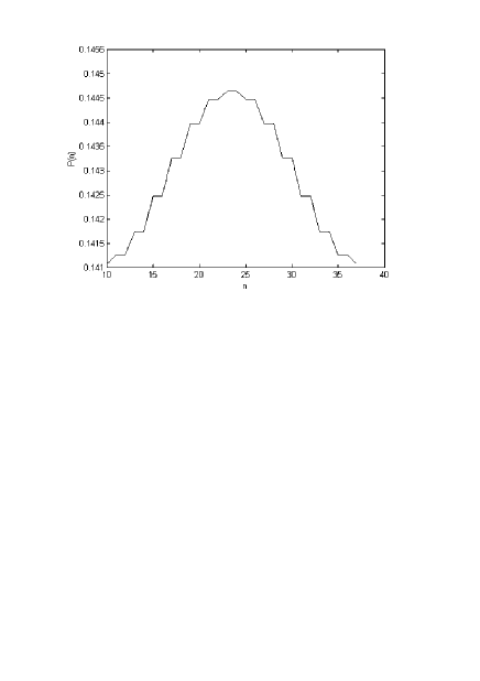
Figure 13: Results of numerical calculations performed by means of recurrent relations (75).

Table 2: Evolution of populations of non-degenerate levels

Formation of statistical distribution of populations of levels $P(n)$ with a lapse of a large evolution time $t\approx 1000T$ of the system. The result shown in this figure corresponds to the case for which the level population creeping is not restricted by condition (34).

At that, the closed system consists of two subsystems: the classical variable field (36) that plays the role of ”a thermostat” with an infinitely high temperature and the quantum pendulum (7). A weak (indirect) interaction of the subsystems produces passages between non-degenerate levels. After a lapse of time $t\gg T$ this interaction ends in a statistical equilibrium between the subsystems. As a result, the quantum pendulum subsystem acquires the thermostat temperature, which in turn leads to the equalization of level populations. The equalization of populations usually called the saturation of passages can be interpreted as the acquisition of an infinite temperature by the quantum pendulum subsystem.

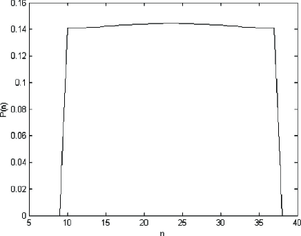
Figure 14: Results of numerical calculations performed by means of recurrent relations (75).

With a lapse of a large time interval $t\approx 1000T$ the formation of stationary distribution of populations among levels takes place. By computer calculations it was found that in the stationary state all $N$ levels satisfying condition (34) were populated with equal probability $1/N$.

I.7 Analogy between the classical and the quantum consideration.

The quantum-mechanical investigation of the universal Hamiltonian (mathematical pendulum), which is reduced to the investigation of the Mathieu-Schrodinger equation, showed that on the plane $(E,2l)$ there exist three areas $G_{+},~{}G_{-}$ and $G$ (see Fig. 8 and 9) differing from each other in their quantum properties. Motion in the area of degenerate states $G_{-}$ is a quantum analog of rotating motion of the pendulum, while motion in the area of degenerate states $G_{+}$ is an analog of oscillatory motion of the pendulum. The area $G$ lying between $G_{-}$ and $G_{+}$ can be regarded as a quantum analog of the classical separatrix. The main quantum peculiarity of the universal Hamiltonian is the appearance of branching and merging points along energy term lines. Branching and merging points define the boundaries between the degenerate areas $G_{\pm}$ and the non-degenerate area $G$. If the system defined by the universal Hamiltonian is perturbed by a slowly changing periodic field, then on the plane $(E,2l)$ the influence of this field produces the motion of the system along the Mathieu characteristics. If, moreover, the system is in degenerate areas for a sufficiently long time, then the phase incursion of wave function phases occurs while the system passes through branching points, which leads to the transition from the pure state to the mixed one. As a result of a multiple passage through branching points, the populations creep by energy terms (Fig. 10). The thus obtained mixed state can be regarded as a quantum analog of the classical stochastic layer. The number of levels affected by the irreversible creeping process is defined by the amplitude of the slowly changing field.

The classical mathematical pendulum may have two oscillation modes (rotational and oscillatory), which on the phase plane are separated by the separatrix (see Fig. 15 a).

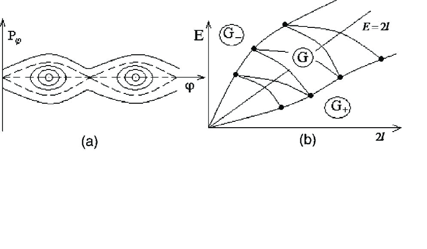
Figure 15: Analogy between the classical and quantum considerations. Unperturbed motion. a) Classical case. Phase plane. Separatrix; b) Quantum case. Specific dependence of the energy spectrum on the parameter (Mathieu characteristics). Degenerate $G_{\pm}$ and non-degenerate $G$ areas of the spectrum.

On the plane $(E,2l)$ the quantum pendulum has two areas of degenerate states $G_{-}$ and $G_{+}$. Quantum states from the area $G_{-}$ possesses translational symmetry in the pendulum phase space. These states are analogous to the classical rotational mode. Quantum states from the degenerate area $G_{+}$ possess symmetry with respect to the equilibrium state of the pendulum (see axis in Fig. 1) and therefore are analogous to the classical oscillatory state. On the plane $(E,2l)$, the area of non-degenerate states $G$, which lies between the areas $G_{+}$ and $G_{-}$, contains the line $E=2l$ corresponding to the classical separatrix (see Fig. 15 b). If the classical pendulum is subjected to harmonically changing force that perturbs a trajectory near to the separatrix, then the perturbed trajectory acquires such a degree of complexity that it can be assumed to be a random one. Therefore we say that a stochastic motion layer (so-called stochastic layer) is formed in the neighborhood of the separatrix (see Fig.16 a). In the case of quantum consideration, the periodic perturbation (36) brings about passages between degenerate states. As a result of repeated passages, before passing to the area $G$ the system gets self-chaotized, passes from the pure state to the mixed one and further evolves irreversibly. While it repeatedly passes through the branch points, the redistribution of populations by the energy spectrum takes place. Only the levels whose branch points satisfy condition (34), participate in the redistribution of populations (see Fig.16 b).

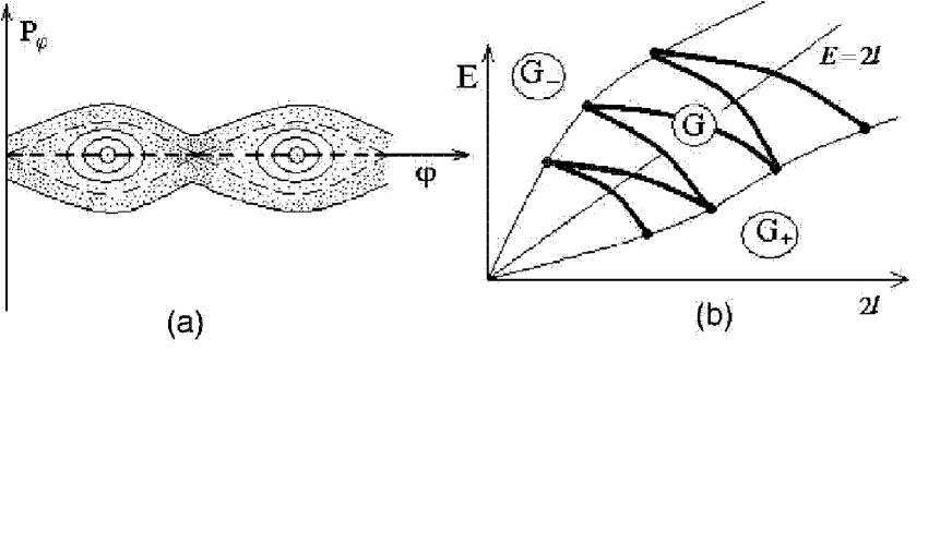
Figure 16: Analogy between the classical and quantum considerations. Perturbed motion: a) Classical case. Stochastic trajectories in the neighborhood of the separatrix form the stochastic layer (cross-hatched area); b) Quantum case. The mixed state was formed as a result of population of non-degenerate levels situated on both sides of the classical separatrix.

I.8 Investigation of quantum chaos of internal rotation motion in polyatomic molecules.

Let us consider two limiting cases of a low and a high energy barrier. In the limit of a low barrier $V_{o}\rightarrow 0$, the Mathieu-Schrodinger equation (18) implies the equation for free rotation

$$\frac{d^{2}\psi}{d\varphi^{2}}+\frac{2I}{\hbar^{2}}\varepsilon_{r}\psi=0.$$

From which for the energy spectrum we obtain $\varepsilon_{r}=(\hbar^{2}/2I)r^{2}$, where $r=0,1,2,\dots$ are integer numbers. Using the above-given numerical estimates for the molecule of ethane $C_{2}H_{6}$, we obtain $\varepsilon_{r}\approx 0.21\cdot 10^{-21}r^{2}J$, which corresponds to the cyclic frequency of rotation $\approx 2.0\cdot 10^{12}r^{2}rad/s$. Comparing the expression for energy with the value of the ethane molecule barrier we see that only levels with a sufficiently large quantum number $(r>10)$ are located high above the barrier and it is only for such levels that the considered limit is valid.

In another limiting case of a high barrier $V_{o}$ the rotator is most of the time inside one of the potential wells where it performs torsional motions. In that case $\alpha$ can be treated as a small angle. After expanding the potential energy in the Schrodinger equation (9) into small angles $\cos 2\alpha\approx 1-2\alpha^{2}$, we obtain a quantum equation for the oscillator, whose energy spectrum has the form $\varepsilon_{r}=(r+1/2)\hbar\omega$, where $\omega=n\sqrt{V_{o}/2I}\approx 6.0\cdot 10^{13}rad/s$. For the energy spectrum of small torsional oscillations we obtain $\varepsilon_{r}\approx(r+1/2)\cdot 0.63\cdot 10^{-20}J$. If we compare the obtained expression for the spectrun with the corresponding numerical value of the barrier, then we can see that only the first two levels $\varepsilon_{o}\approx 0.32\cdot 10^{-20}J,$ $\varepsilon_{1}\approx 0.95\cdot 10^{-20}J$ and $\varepsilon_{2}\approx 1.58\cdot 10^{-20}J$ are located in the well but not at a sufficiently large depth that would allow us to assume that passages between them correspond to small oscillations. Thus we can conclude that for internal rotation of the molecule of ethane $C_{2}H_{6}$ the approximation of small oscillations is not carried out sufficiently well, while the approximation of free rotation is carried out for large quantum numbers.

A real quantitative picture of the internal rotation spectrum can be obtained by means of the Mathieu-characteristics when the points of intersection of the line $l=l_{o}$ with the Mathieu- characteristics is projected on to the energy axis (see Fig.17).

These conclusions are in good agreement with experimental data. In particular, in the experiment we observed the infrared absorption by molecules of $C_{2}H_{6}$ at a frequency $\sim 8.7\cdot 10^{12}Hz$ Shimanouchi . For an energy difference between the levels participating in the absorption process we have the estimate $\Delta\varepsilon_{exper}\sim 0.54\cdot 10^{-20}J$. Comparing the experimental result with the energy difference between two neighboring levels in the case of approximation of small oscillations, we obtain

$$\Delta\varepsilon_{o}=2\pi\nu_{o}\hbar,$$

where $\nu_{o}=\frac{3}{2\pi}\sqrt{\frac{V_{o}}{2I}}$ is the frequency of small oscillations.

Inserting the parameters values for molecules of $C_{2}H_{6}$, we obtain the estimate $\Delta\varepsilon_{o}=0.63\cdot 10^{-20}J$.

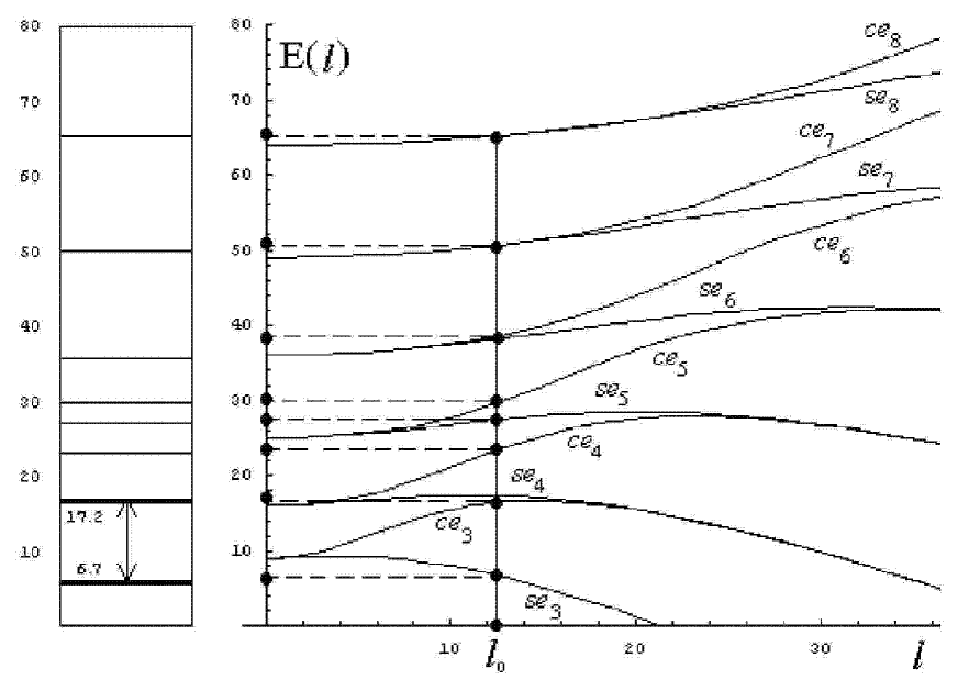
Figure 17: The graphic method of finding energy terms of internal rotation. For the ethane molecule $l_{0}=\frac{2I}{9\hbar^{2}}V_{0}$.

After comparing the obtained estimates with the energy difference between the states described by the wave functions $ce_{3}(\varphi,l_{o}),se_{3}(\varphi,l_{o})$ and applying formula (20), we obtain $\Delta\varepsilon(ce_{3}(\varphi,l_{o})\leftarrow\rightarrow se_{3}(\varphi,l_{o}))\sim 0.54\cdot 10^{-20}J$.

Comparative analysis of the obtained estimates gives us the grounds to conclude that the energy levels corresponding to the states $ce_{3}(\varphi,l_{o}),se_{3}(\varphi,l_{o})$ participate in the infrared absorption revealed in the experiment.

As we see from Fig.17 energy levels involved in the process are distributed in a random manner. In some sense, this resembles RMT. However as number of levels is small, and energy spectrum is well defined.

Let us assume that the considered quantum system is subjected to a radio frequency (RF) monochromatic pumping whose frequency $\Omega$ satisfies the condition $\Omega\ll V_{o}/\hbar$. This causes a slow modulation of quick electron motions in a molecule. The formation of an energy barrier $V_{o}$ is a result of the averaging over quick electron motions and thus it is obvious that due to the pumping effect the barrier value is time-dependent,

$$V_{o}\rightarrow V_{o}+\Delta V\cos\Omega t.$$ (93)

The depth of modulation $\Delta V$ depends on a pumping power. By replacing (76) we obtain the time-dependent Hamiltonian

$$\hat{H}=\hat{H}_{o}(\varphi)+\hat{H}^{\prime}(\varphi,t),$$

$$\hat{H}_{o}(\varphi)=-\frac{\partial^{2}}{\partial\varphi^{2}}+l_{o}\cos 2\varphi,$$ (94)

$$\hat{H}^{\prime}(\varphi,t)=\Delta l\cos 2\varphi\cos\Omega t.$$

$$\Delta l=\frac{2I}{n^{2}\hbar^{2}}\Delta V.$$ (95)

Simple calculations show that the matrix elements of perturbation $\hat{H}^{\prime}(\varphi,t)$ with respect to the wave functions of the nondegenerate area $G$ are equal to zero

$$\langle ce_{n}|\hat{H}^{\prime}(\varphi,t)|se_{n}\rangle\sim\Delta l\int\limits^{2\pi}_{o}ce_{n}(\varphi)\cos 2\varphi se_{n}(\varphi)d\varphi=0,$$ (96)

where $n$ is any integer number. Therefore perturbation (78) cannot bring about passages between nondegenerate levels.

The interaction $\hat{H}^{\prime}(\varphi,t)$, not producing passages between levels, should be inserted in the unperturbed part of the Hamiltonian. The Hamiltonian obtained in this manner can be considered as slowly depending on time.

Thus, in the nondegenerate area the Hamiltonian can be written in the form

$$\hat{H}=-\frac{\partial^{2}}{\partial\varphi^{2}}+l(t)\cos 2\varphi,$$ (97)

Because of the modulation of the parameter $l(t)$ the system passes from one area to another, getting over the branch points.

As different from the nondegenerate state area $G$, in the areas of degenerate states $G_{-}$ and $G_{+}$, the nondiagonal matrix elements of perturbation $\hat{H}^{\prime}(t)$ (78) are not equal to zero. For example, if we take the matrix elements with respect to the wave functions $\psi^{\pm}_{2n+1}$ , then for the left degenerate area $G_{-}$ it can be shown that

$$H^{\prime}_{+-}=H^{\prime}_{-+}=\langle\psi^{+}_{2n+1}|\hat{H}^{\prime}(\varphi,t)|\psi^{-}_{2n+1}\rangle\sim\Delta l\int\limits_{o}^{2\pi}\psi^{+}_{2n+1}\psi^{-\ast}_{2n+1}\cos 2\varphi d\varphi\not=0.$$ (98)

Note that the value $H^{\prime}_{+-}$ has order equal to the pumping modulation (78) depth $\Delta l.$

Analogously to (81), we can write an expression for even $2n$ states as well.

An explicit dependence of $\hat{H}^{\prime}(\varphi,t)$ on time given by the factor $\cos\Omega t$ is assumed to be slow as compared with the period of passages between degenerate states that are produced by the nondiagonal matrix elements $H^{\prime}_{+-}$. Therefore below the perturbation $\hat{H}^{\prime}_{+-}(\varphi,t)$ will be assumed to be the time-independent perturbation that can bring about passages between degenerate states.

In a degenerate area the system may be in the time-dependent superpositional state

$$\psi_{2n}(t)=C^{+}_{n}(t)\psi^{+}_{2n}+C^{-}_{n}(t)\psi^{-}_{2n}.$$ (99)

The probability amplitudes $C^{\pm}_{n}(t)$ are defined by means of the fundamental quantum-mechanical equation, expressing the casuality principle. We write such equations for a pair of doubly degenerate states:

$$-i\hbar\frac{dC^{+}_{n}}{dt}=(E_{on}+H^{\prime}_{++})C^{+}_{n}+H^{\prime}_{+-}C^{-}_{n},$$

$$-i\hbar\frac{dC^{-}_{n}}{dt}=H^{\prime}_{+-}C^{+}_{n}+(E_{on}+H^{\prime}_{--})C^{-}_{n}.$$ (100)

where the matrix elements are taken with respect to degenerate wave functions (see (81)) and $E_{on}$ is the energy of the $n-th$ degenerate level near a branch point.

Let us assume that at the initial moment of time the system was in the degenerate state $\psi^{-}_{2n}$. Then as initial conditions we should take

$$C^{-}_{n}(0)=1,~{}~{}~{}C^{+}_{n}(0)=0.$$ (101)

Having substituted (82) into (81), for the amplitudes we obtain

$$C^{+}_{n}(t)=iexp(\frac{i}{\hbar}Et)\sin\omega t,$$

$$C^{-}_{n}(t)=exp(\frac{i}{\hbar}Et)\cos\omega t,$$ (102)

$$E=E_{on}+H^{\prime}_{\pm\pm},$$

where $\omega=\frac{2\pi}{\tau}=\frac{H^{\prime}_{+-}}{\hbar}$ is the frequency of passages between degenerate states, $\tau$ is the passage time.

Note that the parameter $\omega$ has (like any other parameter) a certain small error $\delta\omega$, which during the time of one passage $t\sim 2\pi/\omega$, leads to an insignificant correction in the phase $2\pi(\delta\omega/\omega)$. However, if during the time $t\sim\Delta T$, when the system is the degenerate area $(\Delta T<T,T=2\pi/\Omega)$ there occurs a great number of passages $(\Delta T\gg\tau)$, then for $\Delta T\delta\omega\approx 2\pi$, a small error $\delta\omega$ leads to the phase uncertainty. Then we say that the phase is self-chaotized. The self-chaotization formed in this manner can be regarded as the embryo of a quantum chaos which, as we will see in the sequel, further spreads to other states.

After a half-period, the system passes to the area of nondegenerate states $G$. In passing through the branch point, there arise nonzero probabilities for passages both to the state $ce_{2n}(\varphi)$ and to the state $se_{2n}(\varphi)$. Thus, in the nondegenerate area the mixed state is formed, which is defined by the density matrix

$$\rho^{ik}_{2n}(t\sim\frac{T}{2}\gg\tau)=\frac{1}{2}\left(\begin{array}[]{cc}1&0\\ 0&1\\ \end{array}\right),\,$$ (105)

where $i$ and $k$ number two levels that correspond to the states $ce_{2n}(\varphi)$ and $se_{2n}(\varphi)$.

As follows from (86), at this evolution stage of the system, the populations of two nondegenerate levels get equalized. It should be noted that though the direct passage (79) between the nondegenerate levels is prohibited, perturbation (78) essentially influences ”indirect” passages. Under ”indirect” passages we understand a sequence of events consisting a passage $G\rightarrow G_{-}$ through the branch point, a set of passages between degenerate states in the area $G_{-}$, and the reverse passage through the branch point $G_{-}\rightarrow G$. The ”indirect” passages occurring during the modulation half period $T/2$ result in the equalization (saturation) of two nondegenerate levels.

Thus ”indirect” passages are directly connected with a quantum chaos. Hence, by fixing ”indirect” passages we thereby fix the presence of a quantum chaos.

Let us assume that the investigated molecule is a component of a substance in a gaseous or liquid state. Then the molecular thermal motion, which tries to establish an equilibrium distribution of populations according to Boltzman’s law, will be a ”competing” process for the quantum chaos described above. Using thermodynamic terminology, we can say that the considered quantum system is located between two thermostats. One of them with medium temperature $T_{o}$ tries to retain thermal equilibrium in the system, while the other, having an infinite temperature, tries to equalize the populations.

An equation describing the change of populations according to the scheme shown in Fig.18 has the form

$$\frac{dn_{i}}{dt}=-2Wn_{i}-\frac{n_{i}-n^{(o)}_{i}}{T_{1}},$$ (106)

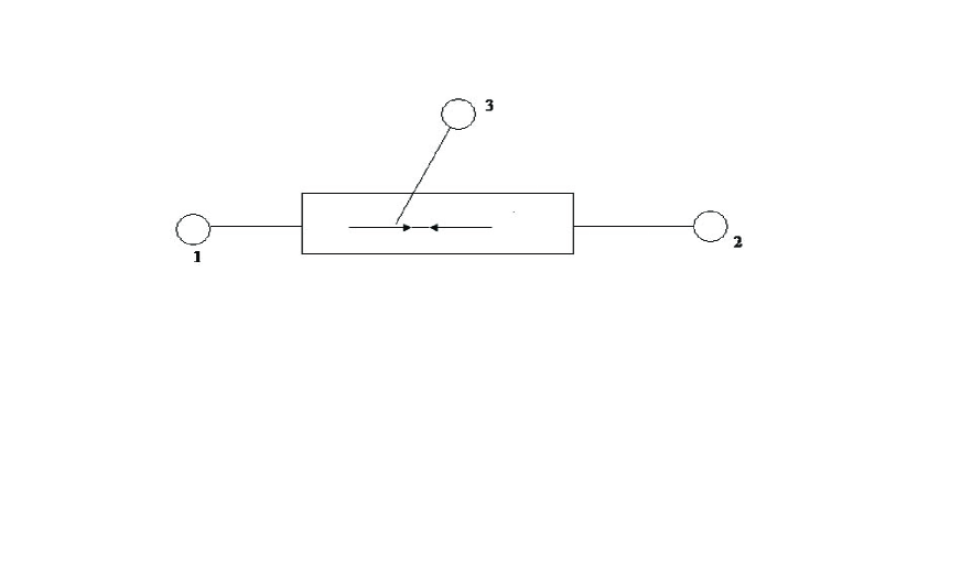
Figure 18: A thermodynamic scheme of the process. Subsystem 1 is a usual thermostat with temperature $T_{0}$ , subsystem 2 is a thermostat having an infinite temperature and consisting of the interaction $\hat{H}^{\prime}(\varphi,t)$ (78); the subsystem 3 is the quantum system corresponding to internal rotations of molecules and being able to receive energy from subsystem 2 and to transfer it to subsystem 1.

where $2W$ is a probability of ”indirect” passages and $T_{1}$ is the time of thermal chaotization. Bloembergen, Parcell and Pound used equation (87) to describe the process of saturation of nuclear magnetic resonance in solid bodies Bloembergen . For a stationary distribution of populations from (87) we obtain

$$n_{i}=n^{(o)}_{i}\frac{1}{1+s},$$ (107)

where $s=2WT_{1}$ is called the saturation parameter. For $s\gg 1$ ”indirect” passages have a stronger effect on the system than thermal processes.

Difference from the magnetic resonance consists in the expression of the transition probability $W$. Whereas, in the case of magnetic resonance, transition probability $2W\sim H^{2}_{1}/\Delta$ is proportional to the pumping intensity $H_{1}$ and inversely proportional to the line width $\Delta$, in the case of non-direct transitions, transition probability $2W\sim 1/T$ does not depend on the oscillation amplitude $\Delta V$ and is inversely proportional to the oscillation period $T$ (i.e. to the time of motion between branch points). But, it is worth to keep in mind, that the amplitude of oscillation must be large enough for the system to achieve the branch points.

Thus, along with the conditions that the perturbation is adiabatic $\Omega\ll V_{0}/\hbar$, phase incursion $\Delta T\gg\tau$ and self-chaotization during the process of multiple transitions between the degenerated states takes place $\Delta T\delta\omega\approx 2\pi,~{}\delta\omega\ll\omega,~{}\Delta T<T$. the condition $s\gg 1$ is a necessary condition for the formation of a quantum chaos. In the opposite limiting case $s\ll 1,~{}n_{i}\approx n_{i}^{(0)}$, the quantum chaos will be completely suppressed by thermal motion. Let us proceed to discussing the quantum chaos possible experimental observation. The most suitable material for this purpose in our opinion is ethane $C_{2}H_{6}$. But, by use of easy estimations one can prove, that for the ethane in the gaseous state, conditions of the quantum chaos observation hardly can be achieved. Really the requirement that modulation must be slow $\Omega\ll V_{0}/\hbar\approx 10^{14}sec^{-1}$, leads to the necessity to take the modulation frequency from the transition radio frequency range $\Omega\approx 0.3\cdot 10^{12}sec^{-1}.$

In the case of gases the thermal chaotization time is estimated by the formula $T_{1}\approx\frac{d}{\bar{\nu}}$ , where $d$ is the molecule size, $\bar{\nu}=\sqrt{\bar{\nu^{2}}}=\sqrt{3/2}(2kT_{0}/m)^{1/2}$ is a mean motion velocity of molecules. After substituting the numerical values for $C_{2}H_{6}$, we obtain $T_{1}\approx 0.3\cdot 10^{-11}\sqrt{1/T_{0}},~{}T_{0}\approx 200^{0}K>184^{0}K$, (where $184^{0}K$ is the boiling point of the ethane at normal pressure). Then for the time of thermal chaotization and for the saturation parameter we get respectively: $T_{1}\approx 0.3\cdot 10^{-12}sec,~{}S\sim(T_{1}/T)\sim 1$. Hence, thermal chaotization and quantum chaos are equally manifested in the system.

In the case of a liquid under $T_{1}$ we should understand the mean time of the settled life of a molecule, which is about $10^{-8}sec$. Relatively large times of relaxation in liquids ensure the fulfillment of the saturation condition $(s\approx T_{1}/T\approx 10^{4})$. In such a way, for ethane $C_{2}H_{6}$ in the liquid state, quantum chaos caused by the non-direct transitions has stronger influence upon the system then common thermal chaotization. At the same time, the state with the equally populated levels will be formed in the system.

Suppose, the system (ethane in the liquid state) is subjected to the action of a infrared radiation field and infrared absorption at the frequency $\sim 289sec^{-1}$ is observed Shimanouchi . This absorption corresponds to the transitions between the states $se_{3}\leftrightarrow ce_{3}$. Furthermore, let us suppose that along with the infrared, the radio frequency pumping which can cause the non-direct transitions is applied. This in its turn leads to the discontinuance of the infrared absorption. This phenomenon can be considered as an observation of quantum chaos.

Now we consider the example of the reaction of isomerization $LiCH\rightleftarrows CHLi$, that was discussed in subsection $E$. As was mentioned above the most simplified model, corresponding to this process, can be presented with the aid of Mathieu-Schrodinger equation (77). It is known, that energy barrier of transition of the process of vibration of the atom $Li$ in the process of isomerization $V\simeq 7\cdot 10^{-20}J$. The moment of inertia is $I_{Li}=1.1\cdot 10^{-46}mcg^{2}$ That is why, in the case $\frac{V_{0}}{\hbar\omega_{0}}=\sqrt{2V_{0}I_{Li}}\approx 19$ number of vibration energy levels are packed in the potential well. Now it is not hard to determine energy spectrum with the aid of Mathieu characteristics.

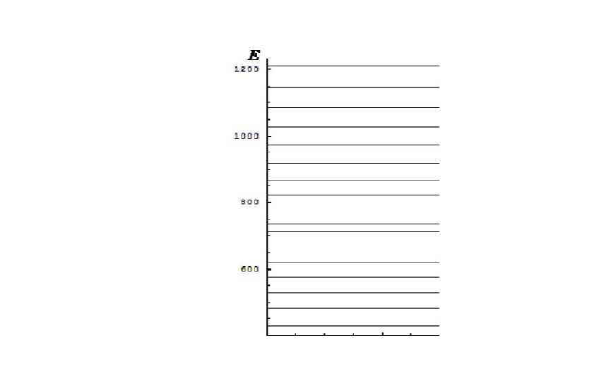
Figure 19: Energy spectrum of the process of isomerization $LiCH\rightleftarrows CHLi$ , obtained as spectrum of eigenvalues of Mathieu-Schrodinger equation, when $l_{0}=\frac{I_{Li}}{2\hbar^{2}}V_{0}\simeq 350.$ Speed of energy levels close to $E=2l_{0}\sim 700$ can easily be observed in figure.

For this process the presence of chaotically distributed levels in infrared region was established with the aid of numerical experiments.

Now let us deal with the problem of nonlinear quantum resonance from which we have begun review. To begin with let us estimate resonance value of $I_{0}$, close to which variation of values of $\Delta I$ may take place. By definition resonance value of action $I_{0}$ is determined from equation $\omega-\omega_{0}+\omega_{n}(I_{0})=0$. By taking typical values of parameters, know from optics: $\omega_{0}\sim 10^{15}sec^{-1},~{}\omega-\omega_{0}\simeq 10^{12}sec^{-1},~{}\gamma\simeq 4\cdot 10^{40}J/kg\cdot m^{4}$ we obtain: $I_{0}=\frac{\omega-\omega_{0}}{\gamma}\frac{2m\omega_{0}^{2}}{3\pi}\simeq 0.5\cdot 10^{-29}J\cdot sec$. This value of action $I/\hbar\simeq 0.5\cdot 10^{5}$ times as much as Plank constant. So, resonance takes place on very high levels (in quasi-classical region) of atoms potential well. As we have done in previous cases, it is possible to find variation spectrum of action $\Delta I$ with the aid of Mathieu characteristics. For this, we must know the value of dimensionless parameter $l_{0}=2V(I_{0})/\omega^{\prime}\hbar^{2}$. It is easy to find the value $\omega^{\prime}\simeq 2\cdot 10^{41}J^{-1}sec^{-2}$ and for strong light fields $f_{0}\simeq 10^{8}V/m$. As a result we obtain $l_{0}\simeq 10^{40}$. This means in its turn, that there are a large number of levels in potential well. Because of the large value of $l_{0}$, it is not possible to determine spectrum by method, used previously, with the aid of Mathieu characteristics. However, by extrapolating it is possible to expect, that at approaching the top of well, alongwith the common attraction of levels, their chaotization will take place. In our opinion, chaotically distributed levels of great density are the basis for random matrix assumption.

II The Peculiarities of Energy Spectrum of Quantum Chaotic Systems. Random Matrix Theory.

In the first part of this work we have considered the possibility of formation of mixed state in quantum chaotic system. The peculiarities of spectral characteristics of the universal Hamiltonian (7) of concrete physical system corresponding to the Mathieu-Schrodinger equation (9) was a cause of this.

In the present part we shall try to get the same results proceeding from more general consideration. In particular, we shall use methods of random matrixes theory Haake ; Stockman ,Gaspard .

Study of quantum reversibility and motion stability is of great interest Hiller . This interest is due to not only the fundamental problem of irreversibility in quantum dynamics, but also to practical application. In particular, it reveals itself in relation to the field of quantum computing Turchett .

A quantity of central importance which has been on the focus of many studies Haug ; Prosen ; Beneti ; Jalabert is the so-called fidelity $f(t)$, which measures the accuracy to which a quantum state can be recovered by inverting, at time $t$, the dynamics with a perturbed Hamiltonian:

$$f(t)=|<\psi|e^{i\hat{H}t}e^{-i\hat{H_{0}}t}|\psi>|^{2},$$ (108)

where $\psi$ is the initial state which evolves in time t with the Hamiltonian $\hat{H_{0}}$ while $\hat{H}=\hat{H_{0}}+V$ is perturbed Hamiltonian. The analysis of this quantity has shown that under some restrictions, the series taken from $f(t)$ is exponential with a rate given by the classical Lyapunov exponent Gaspard . But here a question appears. The point is that the origin of the dynamic stochasticity, which is a reason of irreversibility in classical case, is directly related to the nonlinearity of equations of motion, For classical chaotic system this nonlinearity leads to the repulsion of phase trajectories at a sufficiently quick rate Sagdeev ; Lichtenberg .

In case of quantum consideration, the dynamics of a system is described by a wave function that obeys a linear equation and the notion of a trajectory is not used at all. Hence, at first sight it seems problematic to find out the quantum properties of systems, whose classical consideration reveals their dynamic stochasticity.

In this part of the paper, by using of method of random matrix theory (RMT), we try to show that quantum chaotic dynamics is characterized by the transition from a pure quantum-mechanical state into the mixed one.

With this purpose we shall consider a case when the system’s Hamiltonian may be presented in the form:

$$\hat{H}(t)=\hat{H_{0}}+V(t),$$ (109)

where $\hat{H_{0}}$ is chaotic Hamiltonian with irregular spectrum, $\hat{V}(t+T_{0})=\hat{V}(t)$ periodic in time perturbation. We shall try to show that in this case irreversibility in the system appears as a result of loss of information about the phase factor of the wave function. At the same time, unlike of the second part of the paper where we have proved this fact proceeding from the spectral peculiarities of the concrete system, now we shall prove this in more general manner. For this reason we shall make use of the fact that according to RMT the eigenvalues of chaotic Hamiltonian can be considered as a set of random number Relano ; Retamosa .

After taking (90) into account, the solution of the time-dependent Schrodinger equation

$$i\frac{\partial|\psi(t)>}{\partial t}=\hat{H}(t)|\psi(t)>$$ (110)

can be written formally with the help of a time-dependent exponential Haake

$$U(t)=exp[-i\int_{0}^{t}dt^{\prime}\hat{H}(t^{\prime})],$$ (111)

where the positive time ordering requires:

$$[A(t)B(t^{\prime})]_{t}=\left\{\begin{array}[]{l}A(t)B(t^{\prime})\hskip 19.91684pt{\mbox{i}f}\hskip 5.69046ptt>t^{\prime}\\ B(t^{\prime})A(t)\hskip 19.91684pt{\mbox{i}f}\hskip 5.69046ptt<t^{\prime}\end{array}.\right.$$ (112)

In our case $H(t+T_{0}k)=H(t),~{}~{}k=1,2,\ldots$ the evolution operator referring to one period $T_{0}$, the so-called Flouqet operator $U(T_{0})=F$ Haake , is worthy of consideration, since it yields the stroboscopic view of the dynamics

$$|\psi(kT_{0})>=(\hat{F})^{n}|\psi(0)>.$$ (113)

The Flouqet operator being unitary has unimodular eigenvalues. Suppose we can find eigenvectors $|\varphi_{n}>$ of the Flouqet operator

$$\hat{F}|\varphi_{n}>=e^{-i\varphi_{n}}|\varphi_{n}>,$$

$$<\varphi_{n}|\varphi_{m}>=\delta_{nm}.$$ (114)

Then, with the eigenvalue problem solved, the stroboscopic dynamics may be written explicitly

$$|\psi(kT_{0})>=\sum_{n}e^{-ik\varphi_{n}}<\varphi_{n}|\psi(0)|\varphi_{n}>.$$ (115)

As it was mentioned above, our aim is to prove that one of the signs of the emergence of quantum chaos is a formation of the mixed state. Being initially in a pure quantum-mechanical state, described by the wave function $|\psi>$, the system during the evolution makes an irreversible transition to the mixed state.

The information about whether the system is in the mixed state or in the pure one, may be obtained from the form of the density matrix Feynman . Using (96) as a density matrix of the system we get the following expression:

$$\rho_{nm}(t=kT_{0})=A_{nm}e^{ik(\varphi_{m}-\varphi_{n})},$$ (116)

$$A_{nm}=<\varphi_{m}|\psi(0)><\psi(0)|\varphi_{n}>.$$ (117)

Exponential phase factors of the non-diagonal matrix elements $\rho_{nm}(t)$ express the principle of quantum coherence Schleich , and correspond to the complete quantum-mechanical description of the system in pure quantum-mechanical state. While they are not equal to zero, the system is in the pure state. So, to prove the formation of the mixed state one has to show zeroing of non-diagonal elements of density matrix.

According to the main hypothesis of the random matrix theory Haake , the phase $f(n,m)=\varphi_{m}-\varphi_{n}$ in the exponential factors of the non-diagonal matrix elements in (97) is a random quantity. So, it is clear that the values of matrix elements of density matrix of the chaotic quantum-mechanical system $\rho_{nm}(k)$ are random values too. Taking a statistical average of expression (97), we have

$$<\rho_{nm}(k)>=<A_{nm}e^{ik(\varphi_{m}-\varphi_{n})}>.$$ (118)

Then in case of random phase $f(n,m)$ has a normal dispersion, we get Skrinnikov :

$$\rho_{nm}(k)\sim e^{-\frac{\sigma^{2}k^{2}}{2}}.$$ (119)

This phenomenon is connected with the ”phase incursion”. Uncertainty of phase in (97) is accumulated little by little with time. Finally, when $k>\sqrt{2}/\sigma,$ the uncertainty of phase is of order $2\pi$ , and the phase is completely chaotized. As a result the system passes into mixed state.

According to the theory presented above, calculations were made for concrete physical systems. In particular, in work Skrinnikov chaotic system of connected oscillators was studied, and in work Kereselidze Kepler’s asymmetry problem. The numerical results obtained in these works prove the formula (100) to be correct.

After formation of the mixed state the quantum-mechanical consideration loses its meaning and there is a need to use a kinetic description.

For derivation of master equation let us split the density matrix operator $\hat{\rho}$ on a slow $\hat{\rho}_{R}$ and a fast varying $\hat{\rho}_{NR}$ operators:

$$\hat{\rho}=\hat{\rho}_{R}+\hat{\rho}_{NR}.$$ (120)

Relevant part $\hat{\rho}_{R}$ in the basis $|\phi_{n}\rangle$ contains only diagonal elements, whereas nonrelevant part $\hat{\rho}_{NR}$ contains only nondiagonal elements. These elements, as it was shown in previous section, contain fast oscillating exponents and when taking average over the ensemble, the zeroing of them takes place. Elimination of the diagonal part from the density matrix is linear operation, which satisfies the property of projection operator $\hat{D}^{2}=\hat{D}$ Skrinnikov

$$\hat{\rho}_{R}=\hat{D}\hat{\rho},~{}~{}\hat{\rho}_{NR}=(1-\hat{D})\hat{\rho}.$$ (121)

Let us note that this reflection is nonreversible. Due to the zeroing of nondiagonal part of the density matrix a part of information is lost.

Inasmuch as relevant statistical operator $\hat{\rho}_{R}(t)$ is different from the total operator $\hat{\rho}(t)$, generally speaking it does not suit Liouville-Fon Neumann equation Feynman

$$\frac{\partial\hat{\rho}}{\partial t}+i\hat{L}\hat{\rho}=0,$$ (122)

where $\hat{L}$ is Liouville operator. After acting on the equation (103) with $\hat{D}$ operator, we get

$$\frac{\partial\hat{\rho}_{R}}{\partial t}+i\hat{D}\hat{L}(\hat{\rho}_{R}+\hat{\rho}_{NR})=0,$$ (123)

$$\frac{\partial\hat{\rho}_{NR}}{\partial t}+i(1-\hat{D})\hat{L}(\hat{\rho}_{R}+\hat{\rho}_{NR})=0.$$ (124)

For the purpose to obtain closed equation for $\hat{\rho}_{R}$ we exclude from the equation (104) $\hat{\rho}_{NR}$. As a result we get

$$\frac{\partial\hat{\rho}_{R}(t)}{\partial t}+i\hat{D}\hat{L}\hat{\rho}_{R}(t)+\int^{t}_{t_{o}}K(t-t_{1})\hat{\rho}_{R}(t_{1})dt_{1}=-i\hat{D}\hat{L}exp[-i(t-t_{o})(1-\hat{D})\hat{L}]\hat{\rho}_{NR}(t_{o}),$$ (125)

$$K(t-t_{1})=\hat{D}\hat{L}exp[-i(t-t_{1})(1-\hat{D})\hat{L}](1-\hat{D})\hat{L}.$$ (126)

This equation is valid for $t=\sqrt{2}/\sigma>\tau_{c}$. Evidently $\hat{\rho}_{R}(t)$ is expressed by way of values of $\hat{\rho}_{R}(t_{1})$ taken for the time interval $t_{o}<t_{1}\leq t$, and additionally through the value of $\hat{\rho}_{NR}(t_{o})$. If in the initial moment of time $t=t_{o}$ the system is in a pure quantum-mechanical state, then $\hat{\rho}_{NR}(0)\neq 0$.

In this case solving the equation (107) is problematical. However let us recollect that for $t_{o}>\sqrt{2}/\sigma$ system is already in a mixed state. Therefore equation (107) takes more simple form $(\hat{\rho}_{NR}(0)=0)$

$$\frac{\partial\hat{\rho}_{R}(t)}{\partial t}+i\hat{D}\hat{L}\hat{\rho}_{R}(t)+\int^{t}_{t_{o}}K(t-t_{1})\hat{\rho}_{R}(t_{1})dt_{1}=0.$$ (127)

For solving equation (108) we shall use a method of superoperators Fujita . But before performing this, we should note, that we have obtained a closed equation for relevant part of statistical operator. We were able to come to this only because when $t>t_{o}=\sqrt{2}/\sigma$ the system is in the mixed state and all nondiagonal matrix elements of the density matrix are equal to zero.

Further when studying the evolution of the system we shall consider as the origin of time the moment of the formation of the mixed state in the system. This corresponds to a formal transition to limit $t_{o}\rightarrow-\infty$. Further for simplification of (108) we shall use Abel theorem

$$\lim_{T\rightarrow\infty}\frac{1}{T}\int^{0}_{T}f(t)dt=f(0)-\lim_{\varepsilon\rightarrow+0}\int^{0}_{-\infty}e^{\varepsilon(t^{\prime})}\frac{d}{dt^{\prime}}f^{\prime}(t^{\prime})dt^{\prime}.$$ (128)

Taking (109) into account, equation (108) will have the following form:

$$\frac{\partial\hat{\rho}_{R}(t)}{\partial t}+i\hat{D}\hat{L}\hat{\rho}_{R}(t)=\lim_{\varepsilon\rightarrow+\infty}\int^{t}_{-\infty}e^{\varepsilon(t^{\prime}-t)}K(t-t^{\prime})\hat{\rho}_{R}(t^{\prime})dt^{\prime}.$$ (129)

According to the method of superoperators Nakajima , the correspondence of one operator to another may be considered as representation. The operator in this case will be represented by a matrix element with two indices, while the linear product of operators is a matrix with four indices, i.e. a superoperator Nakajima . A concrete example is the projection of $\hat{D}$ operator on diagonal elements. We should notice, that in our case, the projection operator is some definite physical procedure of averaging matrix elements of the density matrix over Gaussian chaotic ensemble.

From the relation $\hat{D}\rho_{nm}(t)=\rho_{nm}(t)\delta_{mn}$ we come to the following representation of $\hat{D}$ superoperator $\hat{D}_{nmn^{\prime}m^{\prime}}=\delta_{nn^{\prime}}\delta_{mm^{\prime}}\delta_{nn}$ so that

$$\sum_{m^{\prime}n^{\prime}}\hat{D}_{mnm^{\prime}n^{\prime}}\rho_{m^{\prime}n^{\prime}}=\rho_{nm}\delta_{nm}.$$ (130)

Taking (111) into account, (110) is

$$\frac{d\rho_{nn}(t)}{dt}+i\hat{D}(\hat{L}\hat{\rho}_{R})_{nn}=-\int^{0}_{-\infty}dt^{\prime}[K(-t^{\prime})\hat{\rho}_{R}(t+t^{\prime})]_{nn}e^{\varepsilon t^{\prime}}.$$ (131)

In expression (112) and further for short we shall omit $R$ index for diagonal matrix elements of the operator $\hat{\rho}$. Considering the relation

$$[\hat{L},\hat{\rho}_{R}]_{nn}=\sum_{a}L_{nnaa}\rho_{aa}=0$$ (132)

and representing Liouville operator as $L=L_{o}+L^{\prime}$ in compliance with (113) we get

$$\frac{d\rho_{nn}(t)}{dt}=-\int^{t}_{-\infty}dt_{1}e^{\varepsilon(t-t_{1})}\sum_{n}K_{nnmm}(t-t_{1})\rho_{mn}(t_{1}),$$ (133)

and

$$K_{nnmm}(t)=[L^{\prime}e^{-it(1-D)L}(1-D)L^{\prime}]_{nnmm}.$$ (134)

From (115), (114) and from representation of Liouville operator in the form $L=L_{o}+L^{\prime}$, one can see, that kernel $K_{nnmm}(t)$ is at least of second order by $\Delta x_{o}$. Next it is easy to check correctness of the expression

$$\sum_{m}L^{\prime}_{abmm}=\sum_{m}(V_{am}\delta_{bm}-V_{mb}\delta_{am})=V_{ab}-V_{ab}=0,$$ (135)

for Liouville superoperator

$$L_{mnm^{\prime}n^{\prime}}=(H_{mm^{\prime}}\delta_{nn^{\prime}}-H_{nn^{\prime}}\delta_{mm^{\prime}}).$$ (136)

The relation (116) in its turn leads to the rule of sums $\sum_{m}K_{mmnn}=0$. Taking the symmetries $L_{abcd}=L_{cdab},~{}D_{abcd}=D_{cdab}$ into account, from (76) we get Skrinnikov

$$\frac{d\rho_{nn}(t)}{dt}=-\int^{t}_{\infty}dt_{1}e^{\varepsilon(t-t_{1})}\sum_{m\neq n}[K_{nnmm}(t-t_{1})\rho_{mm}(t_{1})-K_{mmnn}(t-t_{1})\rho_{nn}(t_{1})].$$ (137)

Next we shall make the following approximations. With accuracy up to the value of $(\Delta x_{o})^{2}$ order in the exponent in expression (115), we shall replace the complete Liouville operator $\hat{L}=\hat{L}_{0}+\hat{L}^{\prime}$ with $\hat{L}_{0}$. With the same precision we may set $\rho_{nn}(t-t^{\prime})=\rho_{nn}(t)$. As a result from (118) we get

$$\frac{d\rho_{nn}(t)}{dt}=\sum_{m\neq n}[W_{nm}\rho_{mm}(t)-W_{mn}\rho_{nn}(t)],$$ (138)

where

$$W_{nm}=-\int^{o}_{-\infty}dt^{\prime}e^{\varepsilon t^{\prime}}[\hat{L}^{\prime}e^{it(1-\hat{D})\hat{L}_{0}}(1-\hat{D})\hat{L}^{\prime}]_{nnmm}.$$ (139)

Since

$$(\hat{D}\hat{L}_{0})_{abcd}=\delta_{ab}[\Phi_{a}\delta_{ac}\delta_{bd}-\Phi_{b}\delta_{bd}\delta_{ac}]=0,$$ (140)

in expression (120) the operator $\hat{D}$ in the argument of exponential function may be omitted. Taking into account the time dependence of the operator $x(t)=x_{o}\Delta x_{o}f(t),~{}f(t)\sum\limits^{\infty}_{\nu=-\infty}e^{i\nu\Omega t},~{}\Omega=2\pi/T_{o},$ for nondiagonal matrix elements we get Skrinnikov :

$$\frac{d\rho_{nn}(t)}{dt}=\sum_{m\neq n}[W_{nm}\rho_{mm}(t)-W_{mn}\rho_{nn}(t)],$$ (141)

where

$$W_{nm}=\frac{\pi}{2}|V_{nm}|^{2}\sum^{\infty}_{\nu=-\infty}\delta(E_{nm}-\nu\Omega),$$ (142)

is the transition amplitude between the eigenstates of the Hamiltonian $\hat{H}_{o},~{}E_{nm}=\varphi_{n}-\varphi_{m},~{}V_{nm}$ is the matrix element of the operator $\hat{V}_{o}=\Delta x_{o}Q^{2}_{1}Q^{2}_{2}$ in the basic of eigenfunctions of the Hamiltonian $\hat{H}_{o},~{}V_{nm}=\langle\psi_{n}|\hat{V}_{o}|\psi_{m}\rangle$.

Equation (122) describes a nonreversible evolution of the system from nonstationary state to the stationary state defined by the principle of detail equilibrium. To prove irreversibility of the process let us consider time dependence of nonequilibrium entropy Fujita

$$S(t)=-K_{B}\sum_{n}\rho_{nn}(t)ln(\rho_{nn}(t)),$$ (143)

where $K_{B}$ in the Boltzmann constant. Taking into account $\sum_{n}\rho_{nn}(t)=1$, from (124) we get

$$\frac{dS(t)}{dt}=-K_{B}\sum_{n}\sum_{m}W_{nm}[\rho_{mm}(t)-\rho_{nn}(t)]ln(\rho_{nn}(t))-$$

$$-K_{B}\sum_{n}\frac{\partial\rho_{nn}(t)}{\partial t}=\frac{1}{2}K_{B}\sum_{n}\sum_{m}W_{nm}[\rho_{nn}(t)-\rho_{mm}(t)][ln(\rho_{nn}(t))-ln(\rho_{mm}(t))].$$ (144)

Due to the property of logarithmic function

$$(\rho_{nn}(t)-\rho_{mm}(t))(ln(\rho_{nn}(t))-ln(\rho_{mm}(t)))\geq 0,$$ (145)

we see that

$$\frac{dS}{dt}\geq 0$$ (146)

This testifies the growth of entropy during the evolution process.

More exact estimation of entropy growth may be obtained from the principle of detail equilibrium $W_{nm}\rho_{mm}=W_{mn}\rho_{nn}$. Taking into account that in our case $W_{nm}=W_{mn}$, for the entropy growth we get

$$\Delta S=S(t\gg\sqrt{2}/\sigma)-S(t=0)=K_{B}lnN,$$ (147)

where $N$ is the number of levels included into the process.

Thus, we can conclude, that the complex structure of energy spectrum of quantum chaotic system leads to the fact that after averaging over small spread in values of parameters there occurs formation of a mixed sate in the system.

III Conclusion

The traditional notion of an area, where the laws of statistical physics are effective, consists of the assumption that the number of interacting particles is sufficiently large. However, a lot of examples of systems with a small number of degrees of freedom, where chaotic motions occur, had become known by the end of the last century. A new stage in the development of notions about chaos and its origin appeared in the last two decades of the last century. It turned out that the classical Hamiltonian system may experience a special kind of instability. Because of this instability various dynamic characteristics of the system randomly change with time. Such a property of the system that performs random motion is called dynamic stochasticity. It is well known that the appearance of non-reversibility in classical chaotic systems is connected with the local instability of phase trajectories relatively to a small change of initial conditions and parameters of the system. Classical chaotic systems reveal an exponential sensitivity to these changes. This leads to an exponential growth of the initial error with time, and as the result after the statistical averaging over this error, the dynamics of the system becomes non-reversible. In spite of this, the question about the origin of non-reversibility in quantum case remains actual. The point is that the classical notion of instability of phase trajectories loses its sense during quantum consideration. Therefore more detailed analyzes of the possible mechanisms of irreversibility in chaotic quantum-mechanical systems is needed. More over even the fact of possibility of emergence of irreversibility in chaotic quantum-mechanical systems is not evident. Quantum dynamics is unitary and therefore reversible. But on the other hand, without assumption of small initial dispersion of the system’s parameters, classical chaotic dynamics also will be reversible. Note that while studying classical chaos, one usually examines the stability of the system relatively to a small change of initial conditions and system parameters. A small initial error of these parameters always exists and remains unavoidable (one may measure the parameters of the system at a very high precision, but even in this case there is still a small error, the removal of which, i.e. the measurement at absolute precision, is impossible). So not the existence of the unavoidable error is fundamental, but what kind of influence it brings over the system dynamics. It is well known that in case of regular systems such an influence is negligible, but if the system is chaotic, the effect of it increases exponentially. In this review paper we touched upon results obtained in our previous works. We studied paradigmatic model for quantum chaos, time dependent universal Hamiltonian (Hamiltonian of mathematical pendulum). Main result obtained in those works is that reason of irreversibility in time dependent quantum dynamics of the chaotic quantum-mechanical systems, is a very specific spectral characteristic of the system. For universal Hamiltonian and corresponding to it Mathieu-Schrodinger equation above mentioned means very specific dependence of the energy eigenvalues on the values of potential barrier (see. Fig.1). In addition, transition form pure quantum-mechanical state to the mixed one, was found to be quantum analog of the classical chaotic layer, characterized classical chaotic motion near the separatrix. Results obtained are important not only for better understanding of physics of quantum chaos, but for practical implementation to organic molecules, quantum computing and so on.

Acknowledgments

The designated project has been fulfilled by financial support from the Georgian National Foundation (grants: GNSF/STO 7/4-197, GNSF/STO 7/4-179). The financial support of Deutsche Forschungsgemeinschaft SFB 484 under contract number 21095192(EC 94/5-1) is gratefully acknowledged by L. Chotorlishvili.

References

- (1) R.Z. Sagdeev, D.A. Usikov, and G.M. Zaslavsky, Nonlinear Physics,Harwood Academic, New York (1988).
- (2) A.J. Lichtenberg and M.A. Lieberman, Regular and Stochastic Motion, Springer-Verlag, New York (1983).
- (3) K.T. Alligood, T.D. Sauer, and J.A. York, Chaos: An Introduction to Dynamical Systems, Springer, New York (1996).
- (4) M.G. Grifoni and P. Hanggi, Phys.Rep. 304, 229 (1998).
- (5) A. Peres, Phys. Rev.A 30, 1610 (1984).
- (6) P. Jacquod, C. Petitjean arXi 0806.0987 (2008).
- (7) F. Haake, Quantum Signatures of Chaos, Springer, Berlin (2001).
- (8) H.J. Stockman, Quantum Chaos, An Introduction, Cambridge Univ. Press, Cambridge (1993).
- (9) A. Ugulava, L.Chotorlishvili, and K.Nickoladze, Phys.Rev. E 68, 026216 (2003).
- (10) A. Ugulava, L.Chotorlishvili, and K.Nickoladze, Phys.Rev. E 70, 026219 (2004).
- (11) A. Ugulava, L.Chotorlishvili, and K.Nickoladze, Phys.Rev. E 71, 056211 (2005).
- (12) A. Ugulava, L.Chotorlishvili, T. Gvarjaladze, and S.Chkhaidze, Mod.Phys. Lett. B, 21, 415 (2007).
- (13) G.P. Berman, G.M. Zaslavsky, Phys. Lett. A, 61, 295 (1977).
- (14) Janke-Emde-Losh, Tafeln Hoherer Funktionen, Stutgart, 1960.
- (15) H. Bateman, A. Erdelyi, Higher Transcedental Functions, New-York, Toronto, London MC Graw-Hill Book Company INC, 1955.
- (16) M. Hamermesh, Group Theory and its Application to Physical Problems, 1954.
- (17) L.D. Landau and E.M. Lifshitz, Quantum Mechanics, Non-relativistic Theory, Pergamon, Oxford (1977).
- (18) G. Herzberg, Infrared and Raman Spectra of Polyatomic molecules, New York (1945).
- (19) W.H. Flygare, Molecular Stucture and Dinamics (Prentice-Hall, Inc.,Englewood Cliffs, New Jersey,1978).
- (20) R. Essers, J. Tennyson and P.E.S.Wormer, Chemical Physics Letters, 89, 223 (1982).
- (21) F.J. Arranz, F. Borondo, R.M. Benito, The Europian Physical Jornal D 4, 181 (1998).
- (22) F.A. Kaempffer, Concepts in Quantum Mechanics, 1965.
- (23) D. Bohm, Quantum Theory (Prentice-Hall, New-York, 1952).
- (24) T. Shimanouchi, Tables of Molecular Vibrational Frequencies Consolidated, National Bureau of Standards, 1, 1-160 (1972).
- (25) N. Bloembergen, E. Parcell and R. Pound, Phys.Rev.73, 679 (1948).
- (26) P. Gaspard, Chaos, Scattering and Statistical Mechanics, Cambridge Univ. Press, Cambridge (1998).
- (27) M. Hiller, T. Kottos, D. Cohen, T. Geisel, Phys.Rev. Lett. 92, 010402 (2004).
- (28) Q.A. Turchett et al. Phys. Rev. Lett. 7, 4710 (1995).
- (29) F. Haug, M. Bienert, W. Schleich, T. Seligman, M. Raizen, Phys. Rev. A, 71, 043803 (2005).
- (30) T. Prosen, M. Znidaric, J.Phys. A, 35,1455 (2002).
- (31) G. Beneti, G. Casati, Phys. Rev. E 65, 066205 (2002).
- (32) R. Jalabert, H. Pastawski, Phys. Rev. Lett. 86, 2490 (2001).
- (33) A. Relano, J.M. Gomez, R.A. Molina, J. Retamosa and E. Faleiro, Phys.Rev.Lett. 89, 244102 (2002).
- (34) A. Relano, J. Retamosa, E. Faleiro, and J.M. Gomez, Phys.Rev. E 72, 066219 (2005).
- (35) R.P. Feynman, Statistical Mechanics, W.A. Benjaman Inc. Massachusetts (1972).
- (36) W.P. Schleich, Quantum Optics in Phase Space, Wiley-VCH, Berlin (2001).
- (37) L. Chotorlishvili, V. Skrinnikov, Phys.Lett.A, 372, 761 (2008).
- (38) A. Ugulava, L. Chotorlishvili, T. Kereselidze and V. Skrinnikov,Mod. Phys. Lett. B21, 79 (2007).
- (39) S. Fujita, Introduction to Non-Equilibrium Quantum Statistical Mechanics (W.B.Saunders Company, Philadelphia-London, 1966).
- (40) S. Nakajima, Progr.Theor.Phys., 20, 948 (1958).