Fragment Formation in Biased Random Walks

Abstract

We analyse a biased random walk on a 1D lattice with unequal step lengths. Such a walk was recently shown to undergo a phase transition from a state containing a single connected cluster of visited sites to one with several clusters of visited sites (fragments) separated by unvisited sites at a critical probability $p_{c}$ [PRL 99, 180602 (2007)]. The behaviour of $\rho(l)$, the probability of formation of fragments of length $l$ is analysed. An exact expression for the generating function of $\rho(l)$ at the critical point is derived. We prove that the asymptotic behaviour is of the form $\rho(l)\simeq 3/[l(\log\ l)^{2}]$.

1 Introduction

Anteneodo and Morgado recently discussed an interesting one-dimensional random walk model that exhibits a phase transition [1]. In this model, at each time step the random walker moves two lattice spacings to the right or one spacing to the left with probabilities $p$ and $q$ respectively. The sites visited by such a walk are, depending on $p$, either part of a single connected cluster of visited sites or many clusters of visited sites (fragments) separated by single unvisited sites. A transition from one class to the other takes place at the critical probability $p_{c}=1/3$. At large times, for $p<p_{c}$ the cluster of visited sites contains no gaps, however, for $p>p_{c}$ this cluster contains a finite density of unvisited sites. Using Monte-Carlo simulation data, a power law dependence with an exponent $\simeq 1.15$ was estimated for $n(l)$, the fraction of fragments with length $l$. Since the model is a simple one dimensional random walk that is not known to contain any such anamolous exponents, such a behaviour seems unlikely. We prove below that the correct asymptotic behaviour of $n(l)$ at the critical point is $n(l)\sim[l({\textmd{log}}\ l)^{2}]^{-1}$ which is infact hard to distinguish numerically from a power law dependence with exponent $\simeq 1.15$.

At large times, it is easy to see (using the central limit theorem) that the probability distribution of the position of the walker is a Gaussian with mean $\mu(t)=(2p-q)t$ and variance $\sigma^{2}(t)=9pqt$. When the walker is biased towards the left ($p<1/3$), the probability of the walker being on the left of the origin tends to $1$ as $erf(\sqrt{t})$. Hence the visited sites are part of a single connected cluster. When the walker is biased towards the right, in general the clusters of visited sites are separated by single unvisited sites. The fraction of visited sites $f_{v}$ is defined as $S_{n}/L_{n}$ where $S_{n}$ is the average number of distinct sites visited in an $n$-step walk and $L_{n}$ is the average length of an $n$-step walk. The fraction of unvisited sites $f_{u}$, is given by $1-f_{v}$. For this case, $f_{u}$ can be calculated exactly using methods outlined in [3],[1]. In the large $n$ limit, as $\Delta\rightarrow 0^{+}$ , $f_{u}=\Delta+O(\Delta^{2})$, where $\Delta=(p-p_{c})$. The total number of fragments in a walk is equal to the number of unvisited sites and hence $\overline{N}$, the average number of fragments is equal to $L_{n}\Delta$.

The single unvisited sites at the edge of each fragment ensure that the probability of formation of a fragment is independent of the previous history of the walker. The walk can therefore be considered as a discrete process of independent increments where at each step a new fragment of length $l$ is added to the positive edge of the walk with probability $\rho(l)$. These probabilities are multiplicative, i.e.- the probability of formation of a fragment of length $l_{1}$ followed by one of length $l_{2}$ is $\rho(l_{1})\rho(l_{2})$. The number of fragments of length $l$ in a given walk is $N\rho(l)$ where $N$ is the total number of fragments. Therefore $n(l)=\rho(l)/\sum_{l=1}^{\infty}\rho(l)$ and hence $n(l)=\rho(l)$ since $\sum_{l=1}^{\infty}\rho(l)=1$.

2 Determination of fragment formation probability

For a new fragment of length $l$ to be formed the walker must (i) be at the positive edge of the walk ( at site $-1$ for convenience), (ii) hop over site $0$ and reach site $l$ by visiting each site between $1$ and $l$, without visiting sites $0$ and $l+1$. Thus at the end of each step the walker is once again at the positive edge of the walk. $\rho(l)$ is therefore the probability of event (ii) occuring. Hence $\rho(l)$ is the sum of probabilities of all paths that are consistent with (ii).

We calculate $q(l)$, the probability of condition (ii) with the constraint of ‘visiting every site between $1$ and $l$’ relaxed. Hence $q(l)$ is the probability of starting at site $-1$ and reaching site $l$ without visiting $0$ and $l+1$. $q(l)$ thus includes the probability of formation of smaller fragments within the segment $[1,l]$. For example $q(3)=\rho(3)+\rho(1)\rho(1)$. In general

$$q(l)=\rho(l)+\sum_{x_{1}+x_{2}+1=l}\rho(x_{1})\rho(x_{2})+\sum_{x_{1}+x_{2}+x_{3}+2=l}\rho(x_{1})\rho(x_{2})\rho(x_{3})+...$$ (1)

This translates to the following equation involving generating functions

$$\overline{q}(x)=\frac{\overline{\rho}(x)}{1-x\overline{\rho}(x)},\textmd{~{}~{}~{}i.e.-~{}~{}~{}~{}}\overline{\rho}(x)=\frac{\overline{q}(x)}{1+x\overline{q}(x)}\\$$ (2)

where $\overline{\rho}(x)=\sum_{l=1}^{\infty}\rho(l)x^{l}$ and $\overline{q}(x)=\sum_{l=1}^{\infty}q(l)x^{l}$.

2.1 Exact expression for $q(l)$

We calculate $q(l)$ by summing over probabilities of all paths that are consistent with the above definition of $q(l)$. For example, $q(1)$ simply involves the walker reaching site $1$ from $-1$ by hopping over site $0$. Thus $q(1)=p$. It is also easy to see that $q(2)$ is $0$ since unvisited sites in this walk cannot be separated by two lattice sites. In the calculation of $q(3)$ we sum over paths in which the walker starting from $-1$, jumps over site $0$ to reach $1$ and then over $2$ to reach site $3$ with probability $p^{2}$. Once at site $3$, the walker can move two leftward steps followed by a rightward step with probability $pq^{2}$, any number of times, to return to site $3$. Thus $q(3)=p^{2}(1+pq^{2}+(pq^{2})^{2}+...)=p^{2}/(1-pq^{2})$. Generalizing this procedure of summing over all relevant walks, we derive below a closed form expression of $q(l)$ in two equivalent ways.

The walk can be considered as a Markov process where at each time step the walker moves either two lattice spacings to the right or one to the left with probabilities $p$ and $q$ respectively, independent of the previous step. The probability $q(l)$ can be calculated from $P_{l}$, the matrix of transition probabilities [2] with no transitions from the sites $0$, $l+1$ and $l+2$. For example

$$P_{3}=\left[\begin{array}[]{cccccc}0~{}~{}q~{}~{}0~{}~{}0~{}~{}0~{}~{}0\\ 0~{}~{}0~{}~{}q~{}~{}0~{}~{}0~{}~{}0\\ 0~{}~{}0~{}~{}0~{}~{}q~{}~{}0~{}~{}0\\ 0~{}~{}p~{}~{}0~{}~{}0~{}~{}0~{}~{}0\\ 0~{}~{}0~{}~{}p~{}~{}0~{}~{}0~{}~{}0\\ 0~{}~{}0~{}~{}0~{}~{}p~{}~{}0~{}~{}0\\ \end{array}\right]$$ (3)

Where the rows correspond to sites [0 1 2 3 4 5]. Consider the column vector $|p(t)\rangle$ where $\langle s|p(t)\rangle$, the element in row $s$, is the probability of the walker starting at site $1$, being at site $s$ at time step $t$. Now $|p(t)\rangle$ evolves as $|p(t)\rangle=P_{l}^{t}|p(0)\rangle$ which ensures that $|p(t)\rangle$ only contains probabilities of paths that never visit sites $0$ and $l+1$. Since the walker starts at site $1$, $\langle s|p(0)\rangle=\delta_{1,s}$. We calculate $|P\rangle$ where $\langle s|P\rangle$ is the probability of the walker, starting from site $1$ being at site $s$, at any time step. $|P\rangle$ is thus the sum of $|p(t)\rangle$ at every time step. Hence

$$|P\rangle=(I+P_{l}+P_{l}^{2}+...)|p(0)\rangle$$ (4)

All walks that start at $1$ and end at $l$ (at any time step) contribute to $q(l)$, therefore

$$q(l)=p\langle l|(I-P_{l})^{-1}|1\rangle$$ (5)

where $\langle s|1\rangle=\delta_{1,s}$ and $\langle s|l\rangle=\delta_{l,s}$. Thus $q(l)$ is the ($l,1$) matrix element of $p(I-P_{l})^{-1}$. The factor $p$ is present because the walker must hop over site $0$ to reach $1$ as in condition (ii). We thus obtain $q(1)=p$, $q(2)=0$, $q(3)=\frac{p^{2}}{1-pq^{2}}$, $q(4)=\frac{p^{3}q}{1-2pq^{2}}$ and so on. Subtituting these into Eq.(2) we obtain $\rho(1)=p$, $\rho(2)=0$, $\rho(3)=\frac{p^{3}q^{2}}{1-pq^{2}}$, $\rho(4)=\frac{p^{4}q^{2}+3p^{5}q^{4}}{(1-pq^{2})(1-3pq^{2})}$ and so on.

Alternatively, consider $G(s)$, the probability of a walker starting at site -1, being at site $s$ while never visiting $0$ and $l+1$. Now $G(s)$ satisfies the difference equation

$$G(s)=pG(s-2)+qG(s+1)$$ (6)

with the boundary conditions $G(0)=0$ and $G(l+1)=0$. A general solution of $G(s)$ is $Az_{1}^{s}+Bz_{2}^{s}+Cz_{3}^{s}$ which on substitution into Eq.(6) yields the cubic equation $qz^{3}-z^{2}+p=0$. The solutions to this equation are $z=1,z_{\pm}$ where $z_{\pm}=(p\pm\sqrt{p^{2}+4pq})/2q$. By satisfying boundary conditions we obtain

$$G(s)=A[1-\frac{(1-z_{-}^{l+1})}{z_{+}^{l+1}-z_{-}^{l+1}}z_{+}^{s}-\frac{(z_{+}^{l+1}-1)}{z_{+}^{l+1}-z_{-}^{l+1}}z_{-}^{s}]$$ (7)

where A is a constant which is determined from the normalization condition $G(-1)=1$. Alternatively from the definition of $q(l)$ as the connecting probability between $-1$ and $l$ we have

$$q(l)=G(l)/G(-1)$$ (8)

We thus have a closed form expression for $q(l)$. We verify that the two expressions for $q(l)$ are equal as the matrix elements of the column corresponding to site 1 in $p(I-P_{l})^{-1}$ satisfy the same difference equation and, with an appropriate change of variables, the same boundary conditions as G(s).

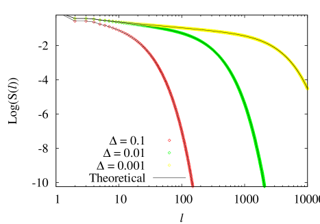
Figure 1: Monte-Carlo plots of $\log(S(l))$ where $S(l)=\sum_{\geq l}n(l)$ for different values of $\Delta=p-p_{c}$ , along with the theoretical curve calculated using Eq.(8) and Eq.(2).

3 Asymptotic behaviour

Away from the critical point $(p>p_{c})$, for large $l$

$$q(l)\simeq\frac{1-\frac{1}{z_{+}}}{1-\frac{1}{z_{-}}}-\frac{z_{-}(z_{+}-z_{-})(z_{+}-1)}{(1-z_{-})^{2}z_{+}^{3}}\textmd{Exp}[-l/\xi]\\$$ (9)

where $\xi=\frac{1}{\log[z_{+}]}\simeq\frac{1}{3(p-p_{c})}$. $\xi$ thus defines a correlation length for $q(l)$ and hence for $\rho(l)$.

At the critical point $q(l)$ simplifies to

$$q(l)=\frac{2[1-(-\frac{1}{2})^{l}]-3l(-\frac{1}{2})^{l}}{8+(-\frac{1}{2})^{l}+6l}\simeq\frac{1}{3l}\textmd{~{}~{}~{}for large $l$}$$ (10)

Therefore as $x\rightarrow 1$ the generating function $\overline{q}(x)$ diverges as $-\frac{1}{3}\log(1-x)$. Hence from Eq.(2)

$$\overline{\rho}(x)=\frac{-\frac{1}{3}\log(1-x)}{1-\frac{x}{3}\log(1-x)}\textmd{~{}~{}~{}for ($x\rightarrow 1,p=p_{c}$)}$$ (11)

Having found the generating function, we can extract the behaviour of $\rho(l)$ for large $l$. From Eq.(11), $\overline{\rho}(x)\simeq 1+3/\log\epsilon$ where $\epsilon=(1-x)$. We can approximate the summation in the generating function by an integral $\overline{\rho}(x)\simeq\int_{1}^{\infty}\textmd{Exp}[-\epsilon\ l]\rho(l)dl$. The singular part of this integral can be evaluated by equating $\overline{\rho}(x)\simeq\int_{1}^{1/\epsilon}\rho(l)dl$ from which we see that $\int_{1/\epsilon}^{\infty}\rho(l)dl\simeq-3/\log\epsilon$. Alternatively, from the fact that the integral $\textmd{Lim}_{\epsilon\rightarrow 0}\int_{2}^{\infty}\textmd{Exp}[-\epsilon\ l]/(\log\ l)^{2}dl$ diverges as $[\epsilon(\log\epsilon)^{2}]^{-1}(1+O[\frac{1}{\log\epsilon}])$ we obtain

$$\rho(l)\simeq\frac{3}{l(\log l)^{2}}\textmd{~{}~{}~{}for large $l$}$$ (12)

We thus have an expression for the asymptotic behaviour of $\rho(l)$.

Cases in which the rightward steps are of length $k>2$ can be treated in a similar way. In this case the independent elements are clusters of visited and unvisited sites separated by $k-1$ zeroes.

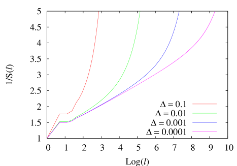
Figure 2: Theoretical plots of $1/S(l)$ v/s Log$(l)$ for different values of $\Delta$ showing a limiting slope of $\simeq$ 0.33 in accordance with Eq.(12)

4 Acknowledgement

I thank Prof. Deepak Dhar for providing the central ideas that led to these results and R. Loganayagam for helpful discussions on the series expansions involved.

References

• [1] C. Anteneodo and W.A.M. Morgado, Phys. Rev. Lett. 99, 180602 (2007)
• [2] W. Feller, Introduction to Probability Theory and Its Applications
• [3] E. W. Montroll and G. H. Weiss, J. Math. Phys. 6, 167 (1965)