An Instability in Triaxial Stellar Systems

Abstract

The radial-orbit instability is a collective phenomenon that has heretofore only been observed in spherical systems. We find that this instability occurs also in triaxial systems, as we checked by performing extensive $N$-body simulations whose initial conditions were obtained by sampling a self-consistent triaxial model of a cuspy galaxy composed of luminous and dark matter. $N$-body simulations show a time evolution of the galaxy that is not due to the development of chaotic motions but, rather, to the collective instability induced by an excess of box-like orbits. The instability quickly transforms such models into a more prolate configuration, with $0.64<b/a<0.77$ and $0.6<c/a<0.7$ for the dark halo and $0.64<b/a<0.77$ and $0.59<c/a<0.67$ for the luminous matter. Stable triaxial, cuspy galaxies with dark matter halos are obtained when the contribution of radially-biased orbits to the solution is reduced. These results constitute the first evidence of the radial-orbit instability in triaxial galaxy models.

1 Introduction

The aim of the current work is to test, by extensive $N$-body simulations, the stationarity of the triaxial galaxy models realized by Capuzzo Dolcetta et al. (2007, hereafter CLMV07). These models were constructed by means of the standard orbital superposition method introduced by Schwarzschild (1979), and represent triaxial, cuspy elliptical galaxies embedded in triaxial dark halos in which the dark and the luminous components have the same axial ratios ($a=1,b=0.86,c=0.7$, i.e., maximal triaxiality). In CLMV07 these models were referred to as MOD1 and MOD1-bis; the only difference between the two solutions was the maximum integration time permitted during the orbital integration, which was longer in MOD1-bis (5 Hubble times) than in MOD1 (2 Hubble times), i.e., MOD1-bis represents a more stationary solution.

2 The Self-Consistent Triaxial Models

The Schwarzschild method used to build the self-consistent solutions consisted in minimizing the discrepancy between the model cell “analytical” masses (obtained by integration of a given $\rho(x,y,z))$ and the masses given by a linear combination of orbits computed in the potential generated by $\rho$. In practice, the quantities to be, separately, minimized are :

$$\chi^{2}_{lum}=\frac{1}{N_{cells}}\sum_{j=1}^{N_{cells}}\left(M_{j;lm}-\sum_{k=1}^{n_{orb}}C_{k;lm}B_{k,j;lm}\right)^{2},~{}$$ (1)

and

$$\chi^{2}_{dm}=\frac{1}{N_{cells}}\sum_{j=1}^{N_{cells}}\left(M_{j;dm}-\sum_{k=1}^{n_{orb}}C_{k;dm}B_{k,j;dm}\right)^{2},~{}$$ (2)

where $B_{k;j;lm(dm)}$ is the fraction of time that the $k$th orbit spends in the $j$th cell of the luminous-matter grid (dark-matter grid); $M_{j;lm}$ is the mass which the model places in the $j$th cell of the luminous-matter grid and $M_{j;dm}$ is the same quantity for the dark-matter grid. $C_{k;lm}$ and $C_{k;dm}$ represent the total mass, respectively, of luminous component and dark matter placed over the $k$th orbit ($1\leq k\leq n_{orb}$). The basic constraints are $C_{k;lm}\geq 0$ and $C_{k;dm}\geq 0$, i.e., non-negative orbit weights.

The mass model considered in CLMV07 for the luminous component was a triaxial generalizations of Dehnen’s spherical model (Dehnen 1993) with a weak cusp. The density law for the luminous component was

$$\rho_{l}(m)=\frac{M}{2\pi a_{l}b_{l}c_{l}}\frac{1}{m(1+m)^{3}}$$ (3)

with

$$m^{2}=\frac{x^{2}}{a_{l}^{2}}+\frac{y^{2}}{b_{l}^{2}}+\frac{z^{2}}{c_{l}^{2}},\qquad 0<c_{l}<b_{l}<a_{l}$$ (4)

and $M$ the total luminous mass.

For the dark component the adopted mass density was

$$\rho_{dm}(m^{\prime})=\frac{\rho_{dm,0}}{(1+m^{\prime})(1+{m^{\prime}}^{2})}$$ (5)

with

$${m^{\prime}}^{2}=\frac{x^{2}}{a_{dm}^{2}}+\frac{y^{2}}{b_{dm}^{2}}+\frac{z^{2}}{a_{dm}^{2}}$$ (6)

and $\rho_{dm,0}$ is the central dark matter density (Burkert 1995). Therefore the dark component has a flat, low-density core. In the present work all quantities are given in units corresponding to $a_{l}=M_{l}=t_{cross}=1$ where $t_{cross}$ is the half mass crossing time of the system. Assuming $M_{l}=10^{11}M\odot$, $a_{l}=1$ kpc and $t_{cross}=26.5$ Myr.

3 N-body initial conditions

In order to study the dynamical properties of MOD1 and MOD1-bis we sampled these models as $N$-body systems and let them evolve. The initial conditions for the $N$-body integrations were set populating the $k$th orbit with a number of particle proportional to $C_{k}$ and randomly choosing positions and velocities from the files containing the results of the orbital integration.

In this work we define $x$($z$)-tube orbits as orbits having a non-vanishing $x$($z$) component of the angular momentum. All other orbits (either box or chaotic) are classified as semi-radial orbits. Regarding the initial conditions of the $N$-body systems, particular care should be given to the direction of rotation of the tube orbits. In fact the persistence of the sense of motion on tubes might be cause of internal streaming motions, giving a “rotating” model (Schwarzschild 1979; Merritt 1980). As a consequence of the symmetries of the potential, the orbits are invariant to a change in sign of the velocity and a decision should be made on the sense of motion of the particles placed on tube orbits. To detect the effects of any rotational motion, and to distinguish them from deformations due to dynamical instabilities, we set two $N$-body simulations for each solutions(MOD1 and MOD1-bis) in the two extreme cases of high and “zero” angular momentum. In Table 1 some parameters of four $N$-body systems, sampling MOD1 and MOD1-bis, are given.

$MODEL$	$Solution$	$L$	$N_{lm}$	$N_{dm}$
$HL$	$MOD1$	$23.71$	$19684$	$144886$
$HL_{bis}$	$MOD1-bis$	$23.58$	$19709$	$146485$
$LL$	$MOD1$	$0.40$	$19684$	$144886$
$LL_{bis}$	$MOD1-bis$	$0.34$	$19709$	$146485$

Table 1: Initial features of models used for the $N$-body simulations. $N_{lm(dm)}$ is the number of particles used to represent the luminous(dark) component; $L$ is the absolute value of the total angular momentum.

4 Results

Simulations reveal that both MOD1 and MOD1-bis evolve in shape, with no particular differences detected between the two cases during the evolution. The variation of the axial ratios is shown in Fig. 1. All the systems were found to have a final quasi-axisymmetric prolate shape. As example, Fig. 2 shows snapshots of the luminous component for model $LL_{bis}$.

We evaluated the anisotropy parameter $2T_{r}/T_{t}$ where $T_{r}=<v_{r}^{2}/2>$ and $T_{t}=<v_{t}^{2}/2>$. For all $N$-body systems, roughlty the same values of the anisotropy parameters were found $[2T_{r}/T_{t}]_{dm}\approx 2$ and $[2T_{r}/T_{t}]_{lm}\approx 1.4$. These values are quite high, in particular for the dark component, suggesting that a bias in the semi-radial orbits may have induced an analog to the radial-orbit instability (ROI) of spherical models.

$\begin{array}[]{cc}\includegraphics[angle={270},width=231.26378pt]{RA_M1_NON.ps}&\includegraphics[angle={270},width=231.26378pt]{RA_M1_PP.ps}\\ \includegraphics[angle={270},width=231.26378pt]{RA_BIS_NON.ps}&\includegraphics[angle={270},width=231.26378pt]{RA_BIS_PP.ps}\end{array}$

Figure 1: Upper panels: evolution of the axial ratios of $HL$(left) and $LL$(right). Lower panels: evolution of the axial ratios of $HL_{bis}$(left) and $LL_{bis}$(right). R is the distance from the center where the axial ratios are evaluated.

5 Minimizing the contribution from semi-radial orbits

To show that the dynamical instability seen in the $N$-body simulations is due to the large radial “pressure” in the models, new solutions containing a lower fraction of semi-radial orbits were computed by means of the orbital superposition technique and then evolved in time as $N$-body systems. Our goal was to demonstrate the existence of a threshold value of the ratio between the number of tube orbits to that of semi-radial orbits above which stability is guaranteed.

Following Poon and Merritt (2004), the relative orbital abundance in the self-consistent models was changed by adding a new term in equations (1) and (2), which become

$$\chi^{2}_{lum}=\frac{1}{N_{cells}}\sum_{j=1}^{N_{cells}}\left(M_{j;lm}-\sum_{k=1}^{n_{orb}}C_{k;lm}B_{k,j;lm}\right)^{2}+{}$$

$$+\sum_{k=1}^{n_{orb}}C_{k;lm}W_{k;lm}~{}~{}~{}~{}~{}~{}~{}~{}~{}~{}~{}~{}~{}~{}~{}~{}~{}$$ (7)

and

$$\chi^{2}_{dm}=\frac{1}{N_{cells}}\sum_{j=1}^{N_{cells}}\left(M_{j;dm}-\sum_{k=1}^{n_{orb}}C_{k;dm}B_{k,j;dm}\right)^{2}+{}$$

$$+\sum_{k=1}^{n_{orb}}C_{k;dm}W_{k;dm}~{}~{}.~{}~{}~{}~{}~{}~{}~{}~{}~{}~{}~{}~{}~{}~{}~{}$$ (8)

As above, the basic constraints were $C_{k;lm}\geq 0$ and $C_{k;dm}\geq 0$ , i.e., non-negative orbit weights.

Here, $W_{k;lm(dm)}$ is the “penalty” associated with the $k$th orbit of the luminous (dark) component, having the effect of filtering the orbital content in the solution: as $W_{k;lm(dm)}$ increases, the mass contribution $C_{k;lm(dm)}$ of the $k$th orbit in the model decreases. We chose $W_{k;lm}=W_{k;dm}=0$ for the tube orbits and $W_{k;lm}\equiv W_{R;lm}>0$ and $W_{k;dm}\equiv W_{R;dm}>0$ for the semi-radial orbits. The new solutions were found by means of the full set of orbits of the MOD1-bis catalog. Four different $N$-body models were obtained by sampling new solutions, taking randomly the sense of rotation for the particles on tube orbits. Each of these models was built using about $20000$ luminous and $150000$ dark matter particles. Table 2 gives the anisotropy of these $N$-body systems: as expected, $[2T_{r}/T_{t}]_{lm}$ and $[2T_{r}/T_{t}]_{dm}$ are decreasing functions of $W_{R}$.

MODEL	$W_{R;lm}$	$W_{R;dm}$	$[2T_{r}/T_{t}]_{lm}$	$[2T_{r}/T_{t}]_{dm}$
$A$	$50$	$50$	$0.512$	$1.175$
$B$	$5$	$5$	$0.784$	$1.335$
$C$	$5\times 10^{-6}$	$5\times 10^{-3}$	$1.220$	$1.754$
$D$	$5\times 10^{-6}$	$50$	$1.230$	$1.174$

Table 2: Anisotropy parameters of the new models.

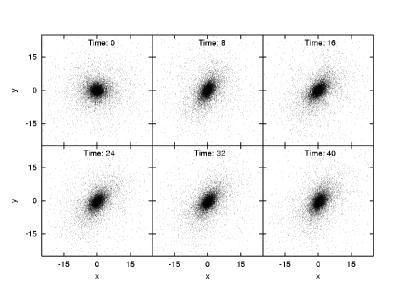
Figure 2: Time evolution of the luminous matter for model $LL_{bis}$, projected onto the $x-y$ plane.

6 The new simulations

$\begin{array}[]{cc}\includegraphics[angle={270},width=231.26378pt]{RA_50tube.ps}&\includegraphics[angle={270},width=231.26378pt]{RA_5tube.ps}\\ \includegraphics[angle={270},width=231.26378pt]{RA_pochetube.ps}&\includegraphics[angle={270},width=231.26378pt]{RA_Ntube.ps}\end{array}$

Figure 3: Evolution of the axis ratios for new models with lower number of semi-radial orbits.

Fig. 3 shows the axis-length evolution of the new models. Model $C$ is clearly dynamically unstable, evolving into a prolate configuration. By contrast, for models $A$, $B$ and $D$, we did not observe the quick transition to instability that characterizes the evolution of models constructed in CLMV07. Therefore, we conclude that the instability can be suppressed when the radial contribution to the solution is reduced. The correlation between the bar formation and the value of the radial velocity dispersion is a clear sign that the dynamical instability, seen above, can be identified with the ROI. Furthermore, the results of model $D$ suggest that the instability disappears when the dark halo gets more isotropic, i.e., the ROI derives mainly by the initial high radial pressure in the dark matter halo.

Finally, we can draw the following conclusions from our analysis of the various different runs:

• The dynamical instability that characterizes the time evolution of the galaxy models built in CLMV07 disappears when solutions contain a smaller number of semi-radial orbits; therefore it can be identified with the ROI;

• The ROI is due to the high concentration of radially “biased” orbits in the dark matter halo. In particular numerical experiments suggest that stable configurations are obtained when $[2T_{r}/T_{t}]_{dm}<1.4$.

7 Discussion

Our study has important implications for future construction of self-consistent models of realistic galaxies. In particular, it has been shown that the dynamical properties of solutions cannot be directly deduced by the Schwarzschild method itself since the temporal development of models can be strongly affected by the distributions in velocity space. In this context, $N$-body tests of the stability of the models seems to be indispensable tool for drawing conclusions about general properties of models constructed via orbital superposition.

Regarding the ROI, because a complete understanding of its mechanism is still lacking, it would be interesting to investigate more in depth its role in the case of triaxial potentials. Our simulations show dynamical features which cannot be detected in the case of spherical symmetry. The method exploited here to change the semi-radial orbit contribution to the models may be useful for constructing other radially-unstable triaxial systems.

References

- [1] Burkert, A. 1995, ApJ, 447, L25
- [2] Capuzzo-Dolcetta, R., Leccese, L., Merritt, D. and Vicari, A. 2007, ApJ, 666, 165 (CLMV07)
- [3] Dehnen, W., 1993, MNRAS, 265, 250
- [4] Merritt, D., 1980, ApJs, 43, 435
- [5] Merritt, D. and Aguilar, L., 1985, MNRAS, 217, 787
- [6] Poon, M. Y. and Merritt, D., 2004, ApJ, 606, 774
- [7] Schwarzschild, M., 1979, ApJ, 232, 236