Theoretical investigation of synchronous totally asymmetric exclusion processes
on lattices with multi-input-single-output junctions

Abstract

In this paper, we investigate the dynamics of synchronous totally asymmetric exclusion processes (TASEPs) on lattices with a multi-input-single-output (MISO) junction, which consists of $m$ subchains for the input and one main chain for the output. An MISO junction is a type of complex geometry, which is relevant to many biological processes as well as vehicular and pedestrian traffic flow. A mean-field approach is developed to deal with the junction that connects the subchains and the main chain. Theoretical calculations for stationary particle currents, density profiles and a phase diagram have been obtained. It is found that the phase boundary moves toward the left in the phase diagram with the increase of the number of subchains. The non-equilibrium stationary states, stationary-state phases and phase boundary are determined by the boundary conditions of the system as well as by the number of subchains. The density profiles obtained from computer simulations show a very good agreement with our theoretical analysis.

PACS numbers: 05.70.Ln, 02.50.Ey, 05.60.Cd

I Introduction

Non-equilibrium transport phenomena have attracted much attention of physicists since physical principles underlying these phenomena could be revealed in terms of phases and phase transitions HELBING01 ; CHOWDHURY05 . Totally asymmetric simple exclusion processes (TASEPs) serve as a basic model for non-equilibrium systems and have been widely applied in the study of transport phenomena in chemistry, physics and biology, for example, particle diffusion through membrane channels CHOU98 , the kinetics of synthesis of proteins SHAW03 , polymer dynamics in dense media SCH99 , gel electrophoresis WIDOM91 , intracellular transport of motor proteins moving along cytoskeletal filaments KLUMPP03 , vehicular traffic CHO00 ; HELBING01 and ant traffic JOHN04 .

TASEPs are non-equilibrium one-dimensional lattice models in which particles move along one direction with hard-core interactions. The exact solution of TASEPs has been obtained by using the matrix product ansatz (MPA) DER98 and the Bethe ansatz SCH01 , respectively. Recently, some extensions of TASEPs focus on coupling with Langmuir kinetics LIPOWSKY01 ; LIPOWSKY03 ; PAR03 ; POPKOV03 ; MIRIN03 ; EVANS03 ; JUH04 ; MUK05 ; NIS05 ; MIT06 and/or lattice geometries PRO04 ; PRO05 ; MIT05 ; STUKALIN06 ; REI06 ; JIANG07 ; WANG07 , as well as bottleneck-induced transport phenomena such as in KLU04 ; PIE06 . Ref. KLU04 investigated diffusive compartments as bottlenecks in a driven transport. They found that when a diffusive bottleneck is at the boundary of a system, the system cannot reach a maximal current phase; when a diffusive bottleneck is in the interior of the system, the system is dictated by the diffusive bottleneck and has a maximal current defined by the bottleneck. More recently, Ref. PIE06 introduced a bottleneck phase to describe the phenomenon that the current is independent of boundary conditions.

In this paper, we focus on one special lattice geometry - junctions, which are widely observed in many real physical systems. Those junctions are formed for various reasons. For example, (i) variation of the number of protofilaments on a microtubule in vitro CHRETIEN92 ; (ii) transport of vesicles in a branching axon or dendrite BURACK00 ; (iii) merging of two or more roads; (iv) data through hubs (e.g., switches, routers) on the Internet. This kind of lattice geometry can cause congestion, e.g., in the traffic of molecular motors, vehicles or data packets. Traffic congestion of molecular motors could lead to some human diseases such as Alzheimers GOLDSTEIN01 and some neurodegenerative diseases HURD96 . Vehicular traffic congestion can pollute environment, increase fuel consumption.

Inspired by this wide range of possible applications, we investigate the dynamics of synchronous (i.e., in parallel update) totally asymmetric exclusion processes on lattices with a multi-input-single-output (MISO) junction (see Fig. 1). The parallel updating procedure has been typically adopted in modeling vehicular and pedestrian traffic CHO00 ; HELBING01 . Multiple inputs exhibit more complex interactions between particles at junction points than two inputs. In reality, it can be observed that several traffic lanes merge into one lane and multiple protofilaments come together to form one protofilament CHRETIEN92 . However, they have not been understood well from the viewpoint of theoretical analysis.

Theoretical calculations, along with a mean-field approximation, are developed. The phase diagram is presented and density profiles are investigated. A phenomenological domain wall theory, based on Refs. ABK98 ; PRO05 , is used to predict phase boundaries. Computer simulations are also conducted. Note that TASEPs on lattices with Y-junctions (e.g., two-input-single-out junctions) in a random updating procedure has been investigated in Ref. PRO05 . Y-junctions can be seen as a special case of multi-input-single-output junctions.

The paper is organized as follows. In Section II, we give a description of a synchronous TASEP model with an MISO junction, theoretical calculations as well as the mean-field approximation are developed. In Section III, we analyze the phase boundaries using a phenomenological domain wall theory. In Section IV, the results of our theoretical calculations and computer simulations are presented. Finally, we give our conclusions in Section V.

II The Model and Mean-field Approximation

An MISO junction is illustrated in Fig. 1. The system consists of $m$ subchains for input and one main chain (chain $m+1$) for output connected by junction points–sites $N$ on the subchains and site $N+1$ on the main chain. Each subchain and the main chain includes $N$ sites. For simplification, inter-lane transitions between subchains are not permitted in this paper. Particles are assumed to move from the left to the right.

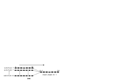
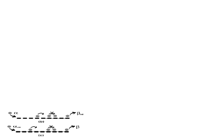
Figure 1: (a) Schematic diagram of a synchronous TASEP with an MISO junction. Particles move from the left to the right with hard-core exclusion. (b) In a subchain, the injection rate at site 1 and the ejection rate at site $N$ are given by $\alpha$ and $\beta_{eff}$, respectively. (c) In the main chain, the injection rate at site $N+1$ and the ejection rate at site $2N$ are given by $\alpha_{eff}$ and $\beta$, respectively.

An occupation variable, $\tau_{\ell,i}$, denotes the state of the $i$th site in the $\ell$th subchain ($\ell=1,2,...,m$) and the main chain ($\ell=m+1$). $\tau_{\ell,i}=1$ (or $\tau_{\ell,i}=0$) means that site $\tau_{\ell,i}$ is occupied (or empty). The system updates all particles in parallel by the following rules (see Fig. 1):

• $i=1$. (i) If $\tau_{\ell,1}=0$, a particle enters the system at rate $\alpha$; or (ii) If $\tau_{\ell,1}=1$ and $\tau_{\ell,2}=0$, then the particle at site $(\ell,1)$ moves into site $(\ell,2)$; or (iii) If both $\tau_{\ell,1}=1$ and $\tau_{\ell,2}=1$, then the particle at site $(\ell,1)$ does not move.

• $i=N$. (i) If sites $N$ of $k$ subchains $(1<k\leq m)$ are occupied by $k$ particles at the same time, particles have the same priority to hop to site $N+1$. However, only one particle will enter site $N+1$ at any single time step, providing that site $N+1$ is empty; or (ii) If only one site $N$ of the subchains is occupied by a particle, the particle can directly hop to site $N+1$ providing that site $N+1$ is empty.

• $i=2N$. If $\tau_{m+1,2N}=1$, the particle leaves the system with rate $\beta$.

• $1<i<N$ or $N+1\leq i<2N$. If $\tau_{\ell,i}=1$, the particle can move into site $(\ell,i+1)$ providing $\tau_{\ell,i+1}=0$. Otherwise, the particle cannot move.

Exactly solvable results of an one-dimensional synchronous TASEP have been obtained in Ref. TIL98 ; GIER99 . We briefly recall these results, as the solution of our synchronous TASEP with a junction can be derived from them. There are three phases (low density (LD), high density (HD) and maximal current(MC)) and a transition line when $\alpha=\beta$. The MC $J=0.5$ can only be reached at $\alpha=\beta=1$ GIER99 .

• When $\alpha<\beta\leq 1$, a low-density (LD) phase is obtained with

  $$J=\rho,\quad\rho=\rho_{1},\quad\rho_{1}=\frac{\alpha}{1+\alpha},\quad\rho_{N}=\frac{\alpha}{\beta(1+a)}.$$ (1)

  where $J$ is the system current; $\rho$ is the bulk density; $\rho_{1}$ ($\rho_{N}$) is the particle density at the first (last) site.

• When $1\geq\alpha>\beta$, a high-density (HD) phase is obtained with

  $$J=1-\rho,\quad\rho=\frac{1}{1+\beta},\quad\rho_{1}=1-\frac{\beta}{\alpha(1+\beta)},\quad\rho_{N}=\rho.$$ (2)

• When $\alpha=\beta<1$, a transition line between LD and HD is obtained.

• When $\alpha=\beta=1$, the maximal current (MC) is obtained and $J=0.5$.

Based on the above results, we develop exactly solvable results for TASEPs with an MISO junction. For an MISO junction, as the current is conserved through the system, we have:

$$J_{1}+J_{2}+\cdot\cdot\cdot+J_{m}=J_{m+1},\quad J_{1}=J_{2}=\cdot\cdot\cdot=J_{m},\quad mJ_{\ell}=J_{m+1}\leq 0.5$$ (3)

where $J_{\ell}$ ($\ell=1,2,...,m$) is the current on the $\ell$th subchain; $J_{m+1}$ is the current of the main chain.

Each of the $m$ subchains of the MISO junction can be seen as a synchronous TASEP with injection rate $\alpha$ and ejection rate $\beta_{eff}$, while the main chain can be seen as a synchronous TASEP with injection rate $\alpha_{eff}$ and ejection rate $\beta$. $\alpha_{eff}$ and $\beta_{eff}$ can be written as

$$\beta_{eff}=1-\rho_{N+1},\quad\alpha_{eff}=m\rho_{N}.$$ (4)

These $m$ subchains should have the identical phases when particles on the $m$ subchains merge into the main chain with the same priority. Our computer simulations also support this prediction. Thus, the stationary state of the system can be obtained by combining the possible phases that exist in each of these subchains and the main chain. As each single chain may have three possible phases (LD, HD and MC), due to the equivalence of these subchains, the number of possible stationary phases of the system is equal to $3^{2}=9$. In other words, a stationary state can be one of the following nine phases: the (LD, LD), (LD, HD), (LD, MC), (HD, LD), (HD, HD), (HD, MC), (MC, LD), (MC, HD), and (MC, MC) phases.

One can see that three phases cannot exist: (MC, LD), (MC, HD) and (MC, MC). According to Eq. (3), it is impossible for the maximal current phase to exist in a subchain since the maximal possible current in the system is no more than 0.5. Therefore, the number of the possible phase combinations reduce to 6, i.e., the (LD, LD), (LD, HD), (LD, MC), (HD, LD), (HD, HD), (HD, MC) phases.

• The (LD, HD) phase. The conditions for this case are as follows:

  $$\alpha<\beta_{eff},\quad\alpha_{eff}>\beta.$$ (5)

  From Eqs. (1) and (2), the stationary properties of this phase are given by:

  $$J_{1}=\frac{\alpha}{1+\alpha},\quad J_{m+1}=\frac{\beta}{1+\beta},\quad\rho_{1}=\frac{\alpha}{1+\alpha},$$

  $$\rho_{N}=\frac{\alpha}{\beta_{eff}(1+\alpha)},\quad\rho_{N+1}=1-\frac{\beta}{\alpha_{eff}(1+\beta)},\quad\rho_{2N}=\frac{1}{1+\beta}.$$ (6)

  According to Eq. (3), $mJ_{1}=J_{m+1}$, we get:

  $$\alpha=\frac{\beta}{m+(m-1)\beta}$$ (7)

  However, $\alpha_{eff}$ and $\beta_{eff}$ are not solvable from above equations. In other words, we cannot calculate the bulk density through the above equations. The density will be solved through the domain wall theory in Section III. From Figs. 2(a) and (b), one can see that $\alpha=\beta/[m+(m-1)\beta]$ (when $\beta<1$) corresponds to the transition line between the (LD, LD) phase and the (HD, HD) phase.

• The (LD, MC) phase. This phase corresponds to the following conditions:

  $$\alpha<\beta_{eff},\quad\alpha_{eff}=\beta=1.$$ (8)

  According to Eqs. (1) and (3), we obtain:

  $$\alpha=\frac{1}{2m-1},\quad J_{1}=\frac{1}{2m},\quad J_{m+1}=0.5.$$ (9)

  Obviously, $\alpha=1/(2m-1)<1/2$ when $m\geq 2$. That is, Eq. (8) is satisfied. Thus, the (LD, MC) phase can exist in the system when:

  $$\alpha=\frac{1}{2m-1},\quad\beta=1.$$ (10)

  Again, we cannot calculate the bulk density through above equations. The density will also be solved through domain wall theory in Section III. From Figs. 2(a) and (b), one can see that the (LD, MC) phase is the transition phase between the (LD, LD), (LD, HD), (HD, HD) and (HD, MC) phases.

• The (LD, LD) phase. The following conditions should be satisfied:

  $$\alpha<\beta_{eff},\quad\alpha_{eff}<\beta.$$ (11)

  According to Eq. (1), the stationary current and density are given by:

  $$J_{1}=\frac{\alpha}{1+\alpha},\quad J_{m+1}=\frac{\alpha_{eff}}{1+\alpha_{eff}},\quad\rho_{1}=\frac{\alpha}{1+\alpha},$$

  $$\rho_{N}=\frac{\alpha}{\beta_{eff}(1+\alpha)},\quad\rho_{N+1}=\frac{\alpha_{eff}}{1+\alpha_{eff}},\quad\rho_{2N}=\frac{\alpha_{eff}}{\beta(1+\alpha_{eff})}.$$ (12)

  Using Eqs. (3) and (4), $\alpha_{eff}$ and $\beta_{eff}$ are expressed as:

  $$\alpha_{eff}=\frac{m\alpha}{1-(m-1)\alpha},\quad\beta_{eff}=\frac{1-(m-1)\alpha}{1+\alpha}.$$ (13)

  Since $\alpha_{eff}\leq 1$ and $\alpha_{eff}=m\alpha/[1-(m-1)\alpha]$, $\alpha\leq 1/(2m-1)$. Substituting Eq. (13) into Eq. (11), we obtain $\alpha<\sqrt{1+m^{2}/4}-m/2$ for $\alpha<\beta_{eff}$, and $\alpha<\beta/[m+(m-1)\beta]$ for $\alpha_{eff}<\beta$. Since $1/(2m-1)<\sqrt{1+m^{2}/4}-m/2$ (when $m\geq 2$) and $\beta/[m+(m-1)\beta]\leq 1/(2m-1)$ (as $\beta\leq 1$), the system is in the (LD, LD) phase when:

  $$\alpha<\frac{\beta}{m+(m-1)\beta},\quad\beta\leq 1.$$ (14)

• The (HD, HD) phase. The conditions for this case are given by:

  $$\alpha>\beta_{eff},\quad\alpha_{eff}>\beta.$$ (15)

  The current and density of this phase in a stationary state are:

  $$J_{1}=\frac{\beta_{eff}}{1+\beta_{eff}},\quad J_{m+1}=\frac{\beta}{1+\beta},\quad\rho_{1}=1-\frac{\beta_{eff}}{\alpha(1+\beta_{eff})},$$

  $$\rho_{N}=\frac{1}{1+\beta_{eff}},\quad\rho_{N+1}=1-\frac{\beta}{\alpha_{eff}(1+\beta)},\quad\rho_{2N}=\frac{1}{1+\beta}.$$ (16)

  From Eqs. (3) and (16), we obtain $\beta_{eff}=\beta/[m+(m-1)\beta]$. Thus, the system is in the (HD, HD) phase when:

  $$\alpha>\frac{\beta}{m+(m-1)\beta}$$ (17)

• The (HD, MC) phase. The corresponding conditions for this phase are:

  $$\alpha>\beta_{eff},\quad\alpha_{eff}=\beta=1.$$ (18)

  According to Eqs. (2-3), we obtain

  $$J_{1}=\frac{1}{2m},\quad\rho_{N}=\frac{1}{m},\quad\rho_{N+1}=\frac{2m-2}{2m-1},\quad\beta_{eff}=\frac{1}{2m-1}.$$ (19)

  Thus, the (HD, MC) phase can exist in the system when:

  $$\alpha>\frac{1}{2m-1},\quad\beta=1.$$ (20)

• (HD, LD) phase. The conditions of existence for this phase can be written as

  $$\alpha>\beta_{eff},\alpha_{eff}<\beta.$$ (21)

  The corresponding expressions for stationary current and density are

  $$J_{1}=\frac{\beta_{eff}}{1+\beta_{eff}},\quad J_{m+1}=\frac{\alpha_{eff}}{1+\alpha_{eff}},\quad\rho_{1}=1-\frac{\beta_{eff}}{\alpha(1+\beta_{eff})},$$

  $$\rho_{N}=\frac{1}{1+\beta_{eff}},\quad\rho_{N+1}=\frac{\alpha_{eff}}{1+\alpha_{eff}},\quad\rho_{2N}=\frac{\alpha_{eff}}{\beta(1+\alpha_{eff})}.$$ (22)

  According to Eq. (3), we have

  $$\alpha_{eff}=\frac{m\beta_{eff}}{1-(m-1)\beta_{eff}}.$$ (23)

  From Eqs. (4) and (22), $\alpha_{eff}$ and $\beta_{eff}$ can be rewritten as follows

  $$\alpha_{eff}=\frac{m}{1+\beta_{eff}},\quad\beta_{eff}=\frac{1}{1+\alpha_{eff}}.$$ (24)

Substituting Eq. (24) into Eq. (23), we obtain $\alpha_{eff}=\sqrt{1+m^{2}/4}+m/2-1$ and $\beta_{eff}=\sqrt{1+m^{2}/4}-m/2$. It can be seen that values of $\alpha_{eff}$ and $\beta_{eff}$ are determined by the number of subchains $m$, independent of $\alpha$ and $\beta$. This indicates that the (HD, LD) phase cannot be represented in the $\alpha-\beta$ plane. In other words, the (HD, LD) phase does not exist in the system. In fact, when the subchains are in the high density phase, particles at site $N$ will hop to site $N+1$ at almost each time step, which leads to $\alpha_{eff}\approx 1$. Thus, it is impossible for the main chain to maintain the low density phase.

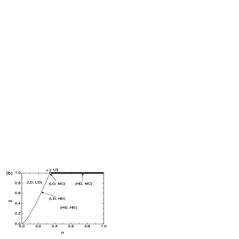
Figure 2: (a) Phase boundaries (or transition lines) for $m=1,2$ and $3$ in the synchronous TASEPs with an MISO junctions. (b) Phase diagram for $m=2$ in the synchronous TASEPs with an MISO junction. The solid line represents the (LD, HD) phase specified by $\alpha=\beta/[m+(m-1)\beta]$ and $\beta<1$; the grey oval corresponds to the (LD, MC) phase specified by $\alpha=1/(2m-1)$ and $\beta=1$; and the black rectangle for the (HD, MC) phase specified by $\alpha>1/(2m-1)$ and $\beta=1$.

From the analysis above, one can see that there are five possible phases ((LD, LD), (LD, HD), (LD, MC), (HD, HD) and (HD, MC)) in this system. Fig. 2(a) shows the possible phase boundaries ($\alpha=\beta/[m+(m-1)\beta]$) for $m=1,2$ and $3$. With the increase of $m$, we can predict that the phase boundary moves toward the left in the phase diagram, which means that the low-density area decreases while the high-density area increases. The phase diagram for $m=2$ is also shown in Fig. 2(b). From Fig. 2(b), one can see that: (i) The (LD, HD) phase corresponds to the transition line between the (LD, LD) phase and the (HD, HD) phase specified by $\alpha=\beta/[m+(m-1)\beta]$ and $0\leq\beta<1$. (ii) The (LD, MC) phase is the transition phase between the (LD, LD),(LD, HD), (HD, HD) and (HD, MC) phases specified by $\alpha=1/(2m-1)$ and $\beta=1$ . Also, note that the transition from the (LD, LD) phase to the (LD, HD) phase, the density change on the subchains is continuous, while the density change on the main chain is discontinuous. Similarly, the transition from the (LD, HD) to the (HD, HD) phases, the density change on the subchains is discontinuous, while the density change of the main chain is continuous. Also, for the transition from the (LD, MC) phase to the (HD, MC) phase, the density change on the subchains is discontinuous, while the density profile on the main chain is unchanged.

From the above analysis, we can see the non-equilibrium stationary states, stationary-state phases and the phase boundary are determined by the boundary conditions of the system as well as by the number of subchains. In other words, the dynamics of the system is determined by its environment and its own structure.

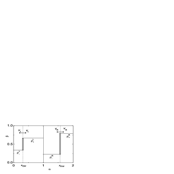
Figure 3: Schematic diagram of the domain wall dynamics in the (LD, HD) phase. The domain wall moves in the left and right subsystems at rates $v_{L}$ and $v_{R}$, respectively.

III Domain Wall Dynamics

A phenomenological domain wall (i.e., shock) theory to explain phase behavior of a TASEP in a random update procedure with open boundaries is introduced in Ref. ABK98 . A domain wall is a phase boundary connected by two possible stationary states. The wall can have a random walk through the system with a drift speed defined as follows ABK98 :

$$V=\frac{J_{+}-J_{-}}{\rho_{+}-\rho_{-}}.$$ (25)

where $J$ and $\rho$ are the currents and densities in the two phases; ’+’(’-’) denotes the phase to the right (left) of the domain wall. When $V>0$, the domain wall moves to the right, while the domain wall travels to the left when $V<0$. For instance, if $\alpha<\beta$ in a TASEP, the domain wall first appears at the left end and will drift to the right later. The wall will pass through the system, which eventually leads to the system being in a low-density stationary state. When $V=0$, it implies that the domain wall has no net drift between two possible phases. In this case, stationary density profiles are linearly increased and the domain wall can exist anywhere with equal probability in the system.

In this paper, the line specified by $\alpha=\beta/[m+(m-1)\beta]$ corresponds to the coexistence of the (LD, LD) and (HD, HD) phases. However, the simple approximation theory may not fully reflect the correlations near the junctions as indicated in Ref. PRO05 . The domain wall theory is adopted in order to derive the phase boundary and the density profile in the bulk. This theory has also been used in Ref. PRO05 .

To determine the position of the domain wall in the system, we define $x$ as $x=i/(2N)$, where $i$ is the site index and $2N$ is the length of the system. In the range of $0<x\leq 1$, the domain wall moves at rate $v_{L}$ in the left subsystem (the sub-chains). In the range of $1<x\leq 2$, the domain wall moves at rate $v_{R}$ in the right subsystem (the main chain), see Fig. (3).

$v_{L}$ and $v_{R}$ can be given by utilizing Eq. (25):

$$v_{L}=\frac{J_{L}}{\rho_{+}^{L}-\rho_{-}^{L}},\quad v_{R}=\frac{J_{R}}{\rho_{+}^{R}-\rho_{-}^{R}}.$$ (26)

where:

$$J_{L}=\frac{\alpha}{1+\alpha},\rho_{+}^{L}=\frac{1}{1+\alpha},\rho_{-}^{L}=\frac{\alpha}{1+\alpha},J_{R}=\frac{\beta}{1+\beta},\rho_{+}^{R}=\frac{1}{1+\beta},\rho_{-}^{R}=\frac{\beta}{1+\beta}.$$ (27)

As a result, $v_{L}$ and $v_{R}$ are rewritten as:

$$v_{L}=\frac{\alpha}{1-\alpha},\quad v_{R}=\frac{\beta}{1-\beta}.$$ (28)

Similarly to Ref. PRO05 , $q_{L}$ ($q_{R}$) is denoted as a probability to find the domain wall at any position in the left (right) subsystem. For a special site, $i$, in the left (right) subsystem, the probability is obviously equal to $q_{L}/N$ ($q_{R}/N$). Then, at the junction point, we have:

$$\frac{v_{L}q_{L}}{N}=\frac{v_{R}q_{R}}{N}.$$ (29)

In addition, normalized $q_{L}$ and $q_{R}$ are satisfied with:

$$q_{L}+q_{R}=1.$$ (30)

Combining Eqs. (29) and (30), we obtain:

$$q_{L}=\frac{v_{R}}{v_{L}+v_{R}},\quad q_{R}=\frac{v_{L}}{v_{L}+v_{R}}.$$ (31)

According to Eq. (28), Eq. (31) implies that:

$$q_{L}=\frac{\beta(1-\alpha)}{\alpha+\beta-2\alpha\beta},\quad q_{R}=\frac{\alpha(1-\beta)}{\alpha+\beta-2\alpha\beta}.$$ (32)

Accordingly, the probabilities of the domain walls falling in certain zones in the left and right subsystems are also given by:

$$Prob(x_{DW}>x)=q_{L}x,\quad 0<x\leq 1,$$ (33)

and

$$Prob(x_{DW}<x)=q_{L}+q_{R}(x-1),\quad 1<x\leq 2.$$ (34)

Thus, the density at any position in the system becomes:

$$\rho(x)_{k}=\rho_{-}^{k}Prob(x_{DW}>x)+\rho_{+}^{k}Prob(x_{DW}<x),\quad k=L,R$$ (35)

Finally, from Eqs. (32)-(35), one can obtain:

$$\rho(x)_{L}=\frac{\alpha}{1+\alpha}+\frac{\beta(1-\alpha)^{2}}{(1+\alpha)(\alpha+\beta-2\alpha\beta)}x,\quad 0<x\leq 1$$ (36)

and

$$\rho(x)_{R}=\frac{\beta}{1+\beta}+\frac{\beta(1-\alpha)(1-\beta)}{(1+\beta)(\alpha+\beta-2\alpha\beta)}+\frac{\alpha(1-\beta)^{2}}{(1+\beta)(\alpha+\beta-2\alpha\beta)}(x-1),\quad 1<x\leq 2.$$ (37)

Densities in the boundary conditions can be calculated as $\rho(x=0)_{L}=\alpha/(1+\alpha)$ and $\rho(x=2)_{R}=1/(1+\beta)$. These results are completely identical with theoretical analysis in Refs. TIL98 ; GIER99 . At the junction point $N$, the densities are equal to $\rho(x=1)_{L}=[\alpha^{2}(1-\beta)+\beta(1-\alpha)]/[(1+\alpha)(\alpha+\beta-2\alpha\beta)],\rho(x=1)_{R}=\beta(1-\alpha\beta)/[(1+\beta)(\alpha+\beta-2\alpha\beta)]$. Note that in the transition line between the (LD, LD) and (HD, HD) phases, we obtain the relationship $\alpha=\beta/[m+(m-1)\beta]$.

IV Simulation results and discussions

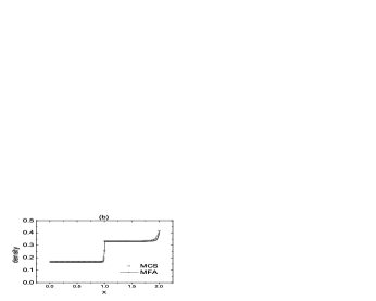
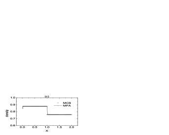
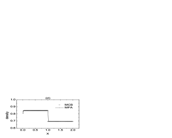
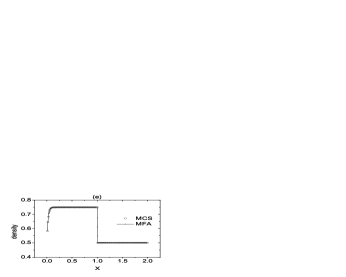
Figure 4: Density profiles obtained from our theoretical calculations and Monte Carlo simulations (MCS) when $m=2$: (a) and (b) are for the (LD, LD) phase, (c) and (d) are for the (HD, HD) phase, and (e) for the (HD, MC) phase. The parameters are set to: (a) $\alpha=0.1$ and $\beta=0.8$, (b) $\alpha=0.2$ and $\beta=0.8$, (c) $\alpha=0.8$ and $\beta=0.32$, (d) $\alpha=0.8$ and $\beta=0.44$, and (e) $\alpha=0.6$ and $\beta=1.0$.

To validate our theoretical analysis, computer simulations are conducted. Here, we only present a synchronous TASEP with a Y-type junction, that is $m=2$. The numbers of sites of the subchains and the main chain are all equal to 1,000. In simulations, stationary density profiles are obtained by averaging $10^{8}$ sampling at each site. The first $10^{5}N$ time steps are discarded to let the transient time out.

The density profiles for the (LD, LD), (HD, HD) and (HD, MC) phases are shown in Fig. 4. We only illustrate the density properties of subchain 1 and the main chain since the density properties of the other subchain is essentially the same as subchain 1. It is found that there is a good agreement between Monte Carlo simulations (MCS) and mean field (MF) analysis (see Figs. 4(a)-(e)), which verifies our theoretical investigations.

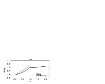
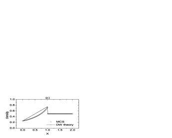
Figure 5: Density profiles obtained by the domain wall (DW) theory and Monte Carlo simulations (MCS) when $m=2$: (a) and (b) for the phase coexistence line between the (LD, LD) and (HD, HD) phases, (c) is for the coexistence phases between the (LD, LD), (LD, HD),(HD,HD)and (HD, MC) phases. The parameters are: (a) $\alpha=0.1$ and $\beta=0.222$, (b) $\alpha=0.2$ and $\beta=0.5$, and (c) $\alpha=1/3$ and $\beta=1.0$.

A phenomenological domain wall (DW) theory developed in Section III is used to calculate the density profiles of phase boundaries such as the (LD, HD) and (LD, MC) phases (see Fig. 5). The results obtained from the domain wall theory show an agreement with computer simulations. When $\alpha$ and $\beta$ both increase and also maintain $\alpha=\beta/[m+(m-1)\beta]$, the system keeps in the (LD, HD) phase until $\beta=1$; the slope of the density profiles for $x<1$ decreases until the slope reduces to 0.5, while the slope of the density profiles for $1<x<2$ also decrease until the slope decreases to 0. For instance, the slope decreases from 0.588 to 0.542 (also see Eq. (32)) when $\alpha$ increases from 0.1 to 0.2 (see Figs. 5(a) and (b)). Finally, the slopes of density profiles of the subchains become 0.5 and the slope of density profile of the main chain becomes 0 when $\alpha=1/3$ and $\beta=1$ (see Fig. 5(c)). Additionally, Monte Carlo simulations, theoretical calculations and domain wall theory all show that, when $\alpha=1/3$ and $\beta=1$ (i.e., the transition phase between the other four phases), the main chain is in the maximal current phase.

Density profiles of the systems for $m=2$ and $m=3$ with the synchronous update scheme are simulated and compared (see Fig. 6). According to Eq. (7), the phase boundary between the (LD, LD) and (HD, HD) phases can be described as $\alpha=\beta/(2+\beta)$ for $m=2$ and $\alpha=\beta/(3+2\beta)$ for $m=3$. Fig. 6 shows that both systems are in the (LD, LD) phase when $\alpha=0.1$ and $\beta=0.8$. However, when $\alpha$ increases (e.g., $\alpha=0.2$), the system for $m=2$ is still in the (LD, LD) phase, while the system for $m=3$ is in the (HD, HD) phase (see Fig. 6(b)). This is due to the phase boundary between the (LD, LD) and (HD, HD) phases moving towards the left when $m$ increases (see Fig. 2(a)). Density profiles in the (HD, HD) phase for both $m=2$ and $m=3$ are shown in Fig. 6(c). Compared with Fig. 6(a) and (c), it can be seen that the density profiles of the subchains of both systems are the same when both systems in the (LD, LD) phase, while the density profiles of the main chains of both systems are the same when both systems are in the (HD, HD) phase. Fig. 6(d) illustrates that the system is in the (LD, LD) phase for $m=2$, while it is in the (HD, MC) phase for $m=3$.

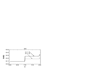
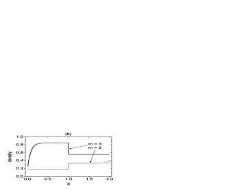
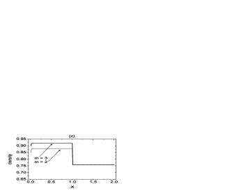
Figure 6: Density profiles in Monte Carlo simulations when $m=2$ and $m=3$. The parameters are: (a) $\alpha=0.1$ and $\beta=0.8$, (b) $\alpha=0.2$ and $\beta=0.8$, (c) $\alpha=0.8$ and $\beta=0.32$, and (d) $\alpha=0.25$ and $\beta=1.0$.

We can also see the similarities and differences between the phase diagram of the system with the synchronous/parallel update scheme (see Fig. 2(b)) and that of the system with the random update scheme (see Fig. 3 in PRO05 ). One can see that the structures of the phase diagrams are similar. All have five phases in their phase diagrams. Also, increasing the number of subchains (i.e., inputs) only shifts the transition line between the (LD, LD) phase and the (HD, HD) phase that does not fall on the boundaries of the phase diagrams. However, the differences in the phase diagrams include: (i) the (HD, MC) phase region in the phase diagram of the system with the random update scheme reduces to a line in that of the system with the synchronous update scheme; and (ii) the line of the (LD, MC) phase in the phase diagram of the system with the random update scheme reduces to a point in the phase diagram of the system with the synchronous update scheme.

Fig. 7 shows the differences in the density profiles of the systems with the synchronous update scheme and the system with the random update scheme when $m=2$. In Fig. 7(a), these two systems are in the (LD, LD) phase when $\alpha=0.1$ and $\beta=0.8$. When $\alpha$ is increased to 0.2 and $\beta$ is unchanged, the system with the synchronous update scheme is still in the (LD, LD) phase, while the phase of the system with the random update scheme becomes the (HD, MC) phase (see Fig. 7(b)). Fig. 7(c) shows the system in the (HD, HD) phase in both systems when $\alpha=0.8$ and $\beta=0.32$. With the increase of $\beta$ (e.g., $\beta=0.8$),the phase of the system with the random update scheme changes to the (HD, MC) phase, while it still keeps in the (HD, HD) phase in the other system.

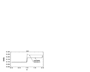
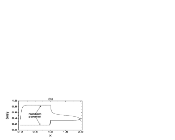
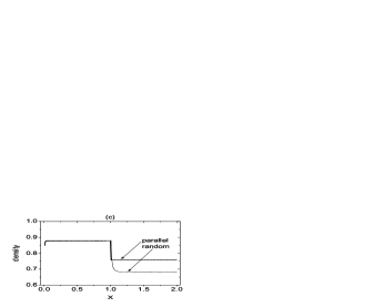
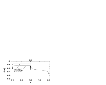
Figure 7: Density profiles in Monte Carlo simulations when $m=2$ in random and parallel updates. The parameters are: (a) $\alpha=0.1$ and $\beta=0.8$, (b) $\alpha=0.2$ and $\beta=0.8$, (c) $\alpha=0.8$ and $\beta=0.32$, and (d) $\alpha=0.8$ and $\beta=0.8$.

Note that the system also exhibits a particle-hole symmetry. Since particles moving forward at junction points with the same priority is equivalent to holes moving backward at the same priority. Also, our method can be used to analyze synchronous TASEPs with a single-input-multi-output (SIMO) junction. Other inhomogeneous synchronous TASEPs can be investigated in the similar way. For instance, it would be interesting to study an MISO junction where these parallel subchains are dynamically different.

V Summary and Conclusions

Multi-input-single-output (MISO) junctions are relevant to many biological processes as well as vehicular and pedestrian traffic flow. Synchronous totally asymmetric exclusion processes (TASEPs) with an MISO junction are investigated in this paper. The theoretical solutions, mean-field approximation, domain wall theory are developed. Extensive computer simulations are conducted. Our theoretical analysis suggests that there are five possible stationary phases ((LD, LD), (LD, HD), (LD, MC), (HD, HD) and (HD, MC)). The (LD, HD) phase corresponds to the transition line (when $\alpha=\beta/[m+(m-1)\beta]$ and $\beta<1$, where $m$ is the number of subchains) between the (LD, LD) phase and the (HD,HD) phase. The (LD, MC) phase (when $\alpha=1/(2m-1)$ and $\beta=1$) is the transition phase between the (LD, LD), (LD, HD), (HD, HD) and (HD, MC) phases. Also, the non-equilibrium stationary state, stationary-state phases and the phase boundary are determined by the boundary conditions of the system as well as the number of subchains. The phase boundary moves to the left in the phase diagram when the number of subchains increases. The density profiles are simulated, which shows good agreement with theoretical analysis.

We also compare the phase diagrams and density profiles between the system with the synchronous update scheme and the system with the random update scheme. The main differences in the phase diagrams include: (i) the (HD, MC) phase region in the phase diagram of the system with the random update scheme reduces to a line in that of the system with the synchronous update scheme; and (ii) the line of the (LD, MC) phase in the phase diagram of the system with the random update scheme reduces to a point in the phase diagram of the system with the synchronous update scheme.

The approach used in this paper can be used directly to analyze TASEPs with a single-input-multi-output (MIMO) junction in a parallel updating procedure.

References

- (1) D. Helbing, Rev. Mod. Phys. 73, 1067 (2001).
- (2) D. Chowdhury, A. Schadschneider and K. Nishinari, Phys. Life. Rev. 2, 318 (2005).
- (3) T. Chou, Phys. Rev. Lett. 80, 85 (1998).
- (4) L.B. Shaw, R.K.P. Zia and K.H. Lee, Phys. Rev. E 68, 021910 (2003)
- (5) G.M. Schütz, Europhys. Lett. 48, 623 (1999).
- (6) B. Widom, J.L. Viovy and A.D. Defontaines, J. Phys. I 1, 1759 (1991).
- (7) S. Klumpp and R. Lipowsky, J. Stat. Phys. 113, 233 (2003).
- (8) D. Chowdhury, L. Santen, and A. Schadschneider, Phys. Rep. 329, 199 (2000).
- (9) A. John, A. Schadschneider, D. Chowdhury and K. Nishinari, J. Theor. Boil. 231, 279 (2004).
- (10) B. Derrida, Phys. Rep. 301, 65 (1998).
- (11) G.M. Schütz, in Phase Transitions and Critical Phenomena, Vol. 19, edited by C. Domb and J.L. Lebowitz (Academic Press, San Diego, 2001).
- (12) R. Lipowsky, S. Klumpp, and T.M. Nieuwenhuizen, Phys. Rev. Lett. 87 , 108101, (2001).
- (13) S. Klumpp and R. Lipowsky, Europhys. Lett. 66, 90, (2004).
- (14) A. Parmeggiani, T. Franosch and E. Frey, Phys. Rev. Lett. 90, 086601 (2003); Phys. Rev. E 70, 046101 (2004).
- (15) V. Popkov, A. Rákos, R.D. Willmann, A.B. Kolomeisky and G.M. Schütz, Phys. Rev. E 67, 066117 (2003).
- (16) N. Mirin and A.B. Kolomeisky, J. Stat. Phys. 110, 811 (2003).
- (17) M.R. Evans, R. Juhász and L. Santen, Phys. Rev. E 68, 026117 (2003).
- (18) R. Juhász and L. Santen, J. Phys. A 37, 3933 (2004).
- (19) S. Mukherji and S.M. Bhattacharjee, J. Phys. A 38, L285 (2005).
- (20) K. Nishinari, Y. Okada, A. Schadschneider and D. Chowdhury, Phys. Rev. Lett. 95, 118101 (2005).
- (21) T. Mitsudo and H. Hayakawa, J. Phys. A 39, 15073 (2006).
- (22) E. Pronina and A.B. Kolomeisky, J. Phys. A 37, 9907 (2004); J. Phys. A 40, 2275 (2007).
- (23) E. Pronina and A.B. Kolomeisky, J. Stat. Mech. P07010 (2005)
- (24) T. Mitsudo and H. Hayakawa, J. Phys. A 38, 3087 (2005).
- (25) E.B. Stukalin and A.B. Kolomeisky, Phys. Rev. E 73, 031922 (2006).
- (26) T. Reichenbach, T. Franosch and E. Frey, Phys. Rev. Lett. 97, 050603 (2006).
- (27) R. Jiang, R.Wang and Q.S. Wu, Physica A 375 (1), 247 (2007).
- (28) R. Wang, M. Liu and R. Jiang, Physica A 387, 457 (2008).
- (29) S. Klumpp and R. Lipowsky, Phys. Rev. E 70, 066104 (2004).
- (30) P. Pierobon, M. Mobilia, R. Kouyos and E. Frey, Phys. Rev. E 74 (3), 031906 (2006).
- (31) D. Chrétien, F. Metoz, F. Verde, E. Karsenti and R.H. Wade, J. Cell Biol. 117, 1031 (1992).
- (32) M.A. Burack, M.A. Silverman and G. Banker, Neuron 26(2), 465 (2000).
- (33) L.S.B. Goldstein, Proc. Nat. Acad. Sci. 98, 6999 (2001).
- (34) D.D. Hurd and W.M. Saxton, Genetics 144, 1075 (1996).
- (35) St.M. Block, L.S.B. Goldstein and B.J. Schnapp, Nature 348, 348 (1990).
- (36) A.B. Kolomeisky, G.M. Schütz, E.B. Kolomeisky and J.P. Straley, J. Phys. A 31, 6911 (1998).
- (37) L.G. Tilstra and M.H. Ernst, J. Phys. A 31, 5033 (1998).
- (38) J. Gier and B. Nienhuis, Phys. Rev. E 59, 4899 (1999).