Jitter radiation images, spectra, and light curves from a relativistic spherical blastwave

Abstract

We consider radiation emitted by the jitter mechanism in a Blandford-McKee self-similar blastwave. We assume the magnetic field configuration throughout the whole blastwave meets the condition for the emission of jitter radiation and we compute the ensuing images, light curves and spectra. The calculations are performed for both a uniform and a wind environment. We compare our jitter results to synchrotron results. We show that jitter radiation produces slightly different spectra than synchrotron, in particular between the self-absorption and the peak frequency, where the jitter spectrum is flat, while the synchrotron spectrum grows as $\nu^{1/3}$. The spectral difference is reflected in the early decay slope of the light curves. We conclude that jitter and synchrotron afterglows can be distinguished from each other with good quality observations. However, it is unlikely that the difference can explain the peculiar behavior of several recent observations, such as flat X-ray slopes and uncorrelated optical and X-ray behavior.

1 Introduction

The synchrotron external shock model (Meszaros & Rees 1997) has been used with great success to model GRB afterglows since their discovery (Wijers, Rees & Meszaros 1997; Piran 1999; Panaitescu & Kumar 2001; Zhang & Meszaros 2004). However, its physical foundations have been put under debate, principally because a coherent equipartition magnetic field is assumed to be generated at the shock front. In addition, the fraction of internal energy that is given to the magnetic field is assumed independent of the location in the blastwave (the distance from the shock) and of the properties of the shock (e.g. its Lorentz factor).

The two latter assumptions have been tested phenomenologically on afterglow data. Rossi & Rees (2003) considered a magnetic field that is allowed to decay behind the shock front. They concluded that afterglow observations require a magnetic field that has an approximately uniform intensity throughout the blastwave (or at least within a distance $R/\Gamma^{2}$ from the shock front). Yost et al. (2003) studied the possibility that the fraction of the internal energy stored in the magnetic field component grows with the decrease of the Lorentz factor of the fireball. They concluded that this effect could explain a sample of radio afterglows that have flat late time radio decay.

Even though these works present interesting constraints on the behavior of the magnetic field, they do not address the mechanism that generates it, its structure, and whether the radiation mechanism is really synchrotron or not. Analytic (Medvedev & Loeb 1999) and numerical work (Silva et al. 2003; Nishikawa et al. 2003; Frederiksen et al. 2004; Medvedev et al. 2005; Spitkovsky 2008; Chang, Spitkovsky & Arons 2008) have started to unveil recently the mechanism by which a magnetic field component is generated behind a relativistic collisionless shock front. All the studies find that the magnetic field is generated through some kind of two-stream instability, such as the Weibel instability (Weibel 1959). Magnetic fields are generated behind the shock with an energy of the order of 30 per cent of the total available internal energy. They are observed to subsequently decay and, possibly, to stabilize at a level of a fraction of a per cent of the internal energy. Whether they decay even further deep into the shocked material is a matter of debate. The structure of the field is observed to be highly tangled and planar behind the shock front and to grow more coherent deep into the blastwave.

The correlation length of the magnetic field right behind the shock is so short that the synchrotron approximations do not hold and a new radiative regime sets in. This form of radiation, called jitter radiation (Medvedev & Loeb, 1999; Medvedev 2000, 2006 or, sometimes, diffusive synchrotron radiation, Fleishman 2006ab), has been studied analytically, semi-analytically and numerically (Medvedev & Loeb 1999; Medvedev 2000; Frederiksen et al. 2004; Medvedev 2006; Fleishman 2006a; Medvedev et al. 2007; Workman et al. 2008). In this work we apply the theory of jitter radiation to compute the emission from a Blandford & McKee (1976) blastwave, taking into account its structure, the special relativistic effects, and the light propagation time. The results include spectra, lightcurves and images, analogously to what is done by Granot, Piran & Sari (1999a) for the synchrotron case.

This paper is organized as follows: In § 2 we describe the numerical methods applied to integrate the radiation spectrum over the BM solution and over surfaces of equal arrival time; in § 3 we describe our results and in § 4 we summarize and discuss them.

2 Modeling The Afterglow

In this section we describe the process by which we solve for the physical shape, evolution, and internal properties of a Gamma-Ray Burst (GRB) blast wave. We loosely follow the outline used by Granot et al. (1999a) but we expand on their work by allowing for both a constant density ISM and a wind environment such as would possibly be found near the progenitor stars of long duration Gamma Ray Bursts. We will describe the physical setup of the problem and then describe the method used to compute images, spectra, and light curves assuming that the whole blastwave radiates jitter radiation. See Medvedev & Loeb (1999), Medvedev (2000) and Workman et al. (2008) for a thorough discussion of the conditions under which jitter radiation is produced.

2.1 The Blandford McKee Solution

To calculate the spectrum of a GRB afterglow emitting jitter radiation we first have to compute the local physical quantities in the blastwave and the time evolution of the afterglow in the relevant geometry of the external medium. As soon as the external shock has swept up a mass comparable to the rest mass of the fireball over its Lorentz factor, the blastwave enters the self-similar stage (Blandford & McKee 1976).

Following Blandford & McKee (1976) we define a similarity variable as:

$$\chi(r)=1+4(4-k)\gamma^{2}_{f}(1-\frac{r}{R})$$ (1)

where $R$ is the radius of the shock, $r$ is the distance to the center of the shock, $\gamma_{f}$ is the Lorentz factor of the material immediately behind the shock front and $k$ describes the properties of the external medium. For a constant density profile, $k=0$, while for a wind environment $k=2$. Using this similarity variable, we can solve for the comoving number density ($n^{\prime}$), the comoving energy density ($e^{\prime}$), and the Lorentz factor ($\gamma$) of the material anywhere within the expanding volume with the following equations:

$$n^{\prime}=4n\gamma_{f}\chi^{\frac{1}{2}}\chi^{\frac{(2k-7)}{(4-k)}},$$ (2)

where $n(r)=n_{ISM}$ for the constant density case and $n(r)=\frac{Ar^{-2}}{m_{p}}$ for the wind environment with $A=\frac{\dot{M}_{w}}{4\pi V_{w}}$ g/cm,

$$e^{\prime}=4nm_{p}c^{2}\gamma_{f}^{2}\chi^{\frac{(4k-17)}{(12-3k)}},$$ (3)

and

$$\gamma=\gamma_{f}\chi^{\frac{-1}{2}}.$$ (4)

To solve for the above quantities, we need to find $\gamma_{f}$, the Lorentz factor of the material directly behind the shock front that defines the blastwave outermost edge. It is given by (e.g., Chevalier & Li, 2000)

$$\gamma_{f}=\left[\frac{(17-4k)E}{16\pi m_{p}n(R)R^{3}c^{2}}\right]^{\frac{1}{2}}.$$ (5)

where $E$ is the energy of the blastwave.

Let us consider now the point $P$ in Fig. 1. It is characterized by a distance $r$ from the center of the explosion and an angle $\theta$ with respect to the line of sight. Velocity at this point is in the $\hat{r}$ direction. The point $P$ begins to emit radiation when it is crossed by the forward shock at the observed time:

$$T_{obs}=\frac{r}{c}\left(1-\cos(\theta)+\frac{1}{4(4-k)\gamma_{f}^{2}}\right)$$ (6)

The radiation observed at time $T_{obs}$ is obtained therefore by integration over the locations $(r,\theta)$ that satisfy:

$$\frac{r}{c}\left(1-\cos(\theta)+\frac{1}{4(4-k)\gamma_{f}^{2}}\right)\leq T_{obs}$$ (7)

At any location that satisfies Eq. 7, the ratio $R/r$ that is needed to compute the self-similar variable $\chi$ is computed through the equation:

$$T_{obs}=\frac{R}{c}\left(1+\frac{1}{4(4-k)\gamma_{f}^{2}}\right)-\frac{r}{c}\cos(\theta)$$ (8)

where $R$ is the radius of the shock at the laboratory time at which the photon was emitted at radius $r$ to be observed at infinity at time $T_{obs}$.

The energy density of the magnetic field and of non-relativistic particles is assumed to be a constant fraction of the local internal energy, as derived from the BM blast wave solution. Such a prescription is analogous to adiabatic evolution of the population of relativistic electrons with the density of particles (Beloborodov 2005). We use the full form for Weibel fields described in detail in Medvedev (2006) and Workman et al. (2008) to describe the geometry and correlation function of the magnetic field. We assume that the properties of the magnetic field stay constant throughout the afterglow and throughout the blast wave. We parametrize the magnitude of the magnetic field according to the usual prescription

$$\frac{\langle B\rangle^{2}}{8\pi}=\epsilon_{B}e^{\prime},$$ (9)

where $\epsilon_{B}$ represents the equipartional fraction of the magnetic field with the energy density.

2.2 The Observed Jitter Spectrum

To determine $P^{\prime}_{\rm tot}(\omega)$, the total power emitted per unit frequency by an ensemble of electrons radiating in a unit volume, we perform the following integral

$$P^{\prime}_{\rm tot}(\omega)=\int_{\gamma_{min}}^{\infty}n^{\prime}(\gamma)p^{\prime}(\omega)d\gamma.$$ (10)

The number density $n$ and the minimum Lorentz factor ($\gamma_{min}$) in the integral are derived by basic assumptions about the total number and energy of electrons, the interested reader is referred to Workman et al. (2008). Once the above quantity has been computed we assume isotropic radiation and, following Rybicki and Lightman (1979), we define the emission coefficient, $j^{\prime}_{\omega}$ as

$$j^{\prime}_{\omega}=\frac{P^{\prime}_{\rm tot}(\omega)}{4\pi}.$$ (11)

Following the process outlined in Medvedev et al. (2007), Workman et al. (2008); Granot, Piran, and Sari (1999b), and Rybicki and Lightman (1979) we define the absorption coefficient as

$$\alpha^{\prime}_{\omega}=\frac{(p+2)\pi^{2}k}{m_{e}\omega^{2}}\int_{\gamma_{min}}^{\infty}\gamma^{-(p+1)}P^{\prime}(\omega)d\gamma.$$ (12)

Once we have found the necessary coefficients we use the fact that $\alpha_{\omega}\omega$ and $\frac{j_{\omega}}{\omega^{2}}$ are both Lorentz invariants with $\omega=\omega^{\prime}\gamma_{b}(1+\frac{v}{c}\cos\theta^{\prime})$; where $\gamma_{b}$ and $v$ refer to the bulk Lorentz factor and velocity of the afterglow and $\cos\theta^{\prime}$ is defined by the angle between a photon’s path and the co-moving volume’s direction. Using this property we can re-write the differential equation for specific intensity in our frame, given by

$$\frac{dI_{\omega}}{ds}=j_{\omega}-\alpha_{\omega}I_{\omega}$$ (13)

directly in terms of comoving quantities. We assume that there is no scattering or frequency redistribution (see Fleishman 2006ab). This allows us to calculate the spectrum by numerically solving for a series of one dimensional, line of sight, integrals. We define our integration region as the three dimensional volume of constant arrival time, which is given by equation 8. As the jitter radiation depends on the angle of emission in the co-moving frame, we solve for $\theta^{\prime}$ using $\theta$ and $\beta$ by inverting the equation

$$cos(\theta)=\frac{cos(\theta^{\prime})+\beta}{1+\beta cos(\theta^{\prime})}$$ (14)

Once we have found the comoving angle at each point, we use the the Blandford-McKee solution to find the values of $\gamma$, $n^{\prime}$, $e^{\prime}$, and the magnetic field at each point and solve for $j^{\prime}_{\omega}$ and $\alpha_{\omega}^{\prime}$.

With these functions known throughout the volume of constant arrival time, we solve the equation for observed specific intensity, at a given frequency, along lines of sight that span the vertical extent of the surface, giving us $I_{\omega}(y)$ where y is the perpendicular distance from the center of the source (see Fig. 1).

Cooling is added analytically by changing the spectral slope to $\omega^{p-2}$ above a frequency of

$$\omega_{c}=\frac{8.5\times 10^{16}}{2\pi}E_{52}^{-1/2}(\frac{\epsilon_{B}}{0.001})^{-3/2}n_{ISM}^{-1}t_{days}^{-1/2}$$ (15)

(from Sari et al. 1998) for the ISM case and

$$\omega_{c}=\frac{5.7\times 10^{15}}{2\pi}E_{52}^{-1/2}(\frac{\epsilon_{B}}{0.001})^{-3/2}A_{*}^{-2}t_{days}^{1/2}$$ (16)

(from Chavalier & Li 2000) for the wind case, where $A_{*}=\frac{A}{3\times 10^{35}~{}cm^{-1}}$. However, for the parameters and times considered in this paper, cooling only becomes important above $32$ keV for the ISM case and $24$ keV for the wind case.

Once we have solved for the specific intensity in the observer frame, the observed flux at the detector is given by

$$F_{\omega}=2\pi\frac{1}{d^{2}}\int_{0}^{R_{\perp,max}}I_{\omega}(y)ydy,$$ (17)

where $d$ is the distance to the afterglow and $R_{\perp,max}$ is the largest perpendicular extent of the afterglow (as in Granot et al. 1999a).

3 Results

In order to compare synchrotron and jitter radiation we calculate the spectrum and time evolution for both radiation mechanisms for the case of a constant (ISM) and a wind external medium, for a total of 4 models. Analytical lightcurves for these models are derived in Medvedev et al. (2007). In all four cases the total isotropic equivalent energy in the blast wave was $E=10^{53}$ erg, the magnetic field equipartition fraction was $\epsilon_{B}=10^{-5}$, and the fraction of internal energy in electrons was $\epsilon_{e}=0.01$. For the ISM case the external density was $n=1$ while for the wind medium we assumed $\dot{M}=10^{-6}M_{\sun}$/yr and $v_{w}=1000$ km/s giving $A_{*}=0.1$.

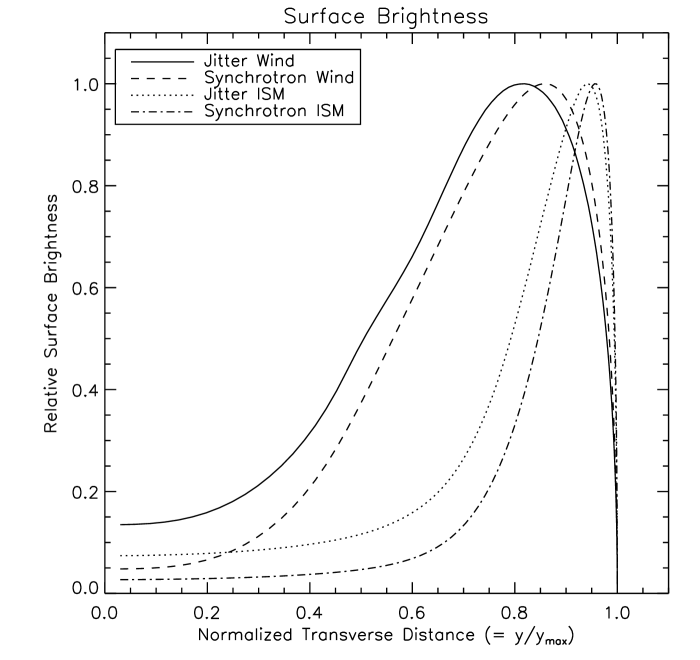
Figure 3: Comparison of surface brightness at $1$ eV at $t=1000$ seconds for the same 4 models of Fig. 2. In all cases, the emission is concentrated towards the outer edge. Normalized transverse distance is defined as $y/y_{max}$ with $y$ defined as in Fig. 1.

A spectrum for each of these 4 models at $t=500$s is plotted in Fig. 2. At this time, the two synchrotron models have a peak frequency of about $0.3$ eV. At lower frequencies the spectrum increases as $\omega^{1/3}$ and at higher frequencies it decreases as $\omega^{-(p-1)/2}$. The self-absorption break is observed at $\sim 10^{-2}$ eV. The two jitter radiation models have similar behavior to the synchrotron models above the peak frequency and in the optically thick regime. However, the jitter models have a nearly flat spectrum below the peak frequency rather than a $\nu^{1/3}$ branch. Even though jitter radiation can produce a spectral slope as steep as $\omega^{1}$ at small angles, the integrated emission is dominated by material at large comoving angles (see Fig. 3) which produce a flat spectrum for jitter radiation (see Medvedev 2006; Medvedev et al. 2007; Workman et. al. 2008). A good quality spectrum over a wide frequency range can distinguish between the synchrotron and jitter radiation mechanisms if the $\nu^{1/3}$ or flat portion of the spectrum is captured. However, the spectrum alone cannot separate ISM and wind external media.

At very low frequency (see Fig. 4) all models are initially optically thick. This results in an increase of luminosity as $t^{1/2}$ for the two ISM models and an increase as $t^{1}$ for the two wind models. The radiation mechanism does not significantly affect the results in the optically thick regime.

At higher frequency all four models are optically thin. A comparison of the light curves for the four models at $1$ eV is shown in Fig. 5. For the ISM case, the synchrotron spectrum initially increases as $t^{1/2}$ and then transitions to a steep decay ($t^{-3(p-1)/4}$) as the peak frequency of the spectrum decreases below $1$ eV. This light curve is similar to the low frequency synchrotron-ISM and jitter-ISM models is Fig. 4. With a wind external medium and synchrotron radiation, the light curve is initially flat before transitioning to a steep decay ($t^{-(3p-1)/4}$). If the jitter radiation mechanism is used, the slope of the light curves are initially decreased by a factor of $t^{-1/2}$, giving a flat initial slope for the jitter-ISM model and a decrease of $t^{-1/2}$ for the jitter-wind case. The result is that in this regime the jitter-ISM and synchrotron-wind models are not distinguishable from each other from the light curve alone, as they both begin with a flat intensity.

For the jitter-wind case, the luminosity initially decreases as $t^{-1/2}$. This gives the light curve the appearance of a broken powerlaw decay. The break occurs at about $10^{3}$s at $1$ eV for this example, but the time of the break depends on frequency as $t_{break}\propto\omega^{-2/3}$. Fig. 6 shows light curves from the jitter-wind model for energies between $10^{-3}$ eV and $1$ keV. The jitter wind model naturally gives rise to a power law decay with a chromatic break between slopes of $t^{-1/2}$ and $t^{-(3p-1)/4}$. At lower frequencies in Fig. 6, the initial slope is increasing as the ejecta are initially optically thick. Observations of the jitter-wind model would show a chromatic break over a range of frequencies or a steep decay at high frequency with a shallow decay and then a break at lower frequencies, depending on the time range and frequencies of the observations.

Fig. 7 shows light curves from the jitter-wind model in the x-ray ($1$ keV), visible ($575$ nm), and radio ($24.2$ GHz). In this case, the x-ray observations show a single powerlaw decay, the visible shows a broken powerlaw, and the radio shows a powerlaw increase.

4 Discussion and conclusions

We have calculated the spectra and light curves produced by jitter radiation from a relativistic fireball expanding into either an ISM (constant density) or wind ($\rho\propto r^{-2}$) external medium including self absorption and electron cooling, and then compared these results to results for synchrotron radiation in identical cases. We improved upon our previous computations (Medvedev et al. 2007) by performing the integration over the blastwave and taking into account the light travel time of the photons.

The primary difference between jitter and synchrotron radiation is that jitter radiation produces a flat spectral slope below the peak frequency, rather than the $\omega^{1/3}$ slope seen in synchrotron radiation. Jitter and synchrotron radiation are not distinguishable in the optically thick regime or above the peak frequency, only in between. The flat spectral slope of jitter radiation has the effect of decreasing the slope of the light curve by a factor of $t^{-1/2}$ compared to synchrotron radiation in the relevant frequency and temporal intervals. This means that the slope of the light curve, while the observed frequency is below the peak frequency, decreases from $t^{1/2}$ for synchrotron to $t^{0}$ for jitter in the ISM case and decreases from $t^{0}$ to $t^{-1/2}$ for the wind case. This indicates that the jitter-ISM and synchrotron-wind cases would not be distinguishable from a single light curve as they both have a $t^{0}$ slope.

In the last four years, Swift observations, combined with ground-based optical and radio telescopes have put the standard synchrotron external shock model under scrutiny. The new observations have shown temporally flat X-ray light curves (Nousek et al. 2006), chromatic breaks (e.g., Huang et al. 2007), and uncorrelated multi-band behavior (e.g., Blustin et al. 2006; Dai et al. 2007). The light curves and spectra of jitter and synchrotron radiation are different. However, the differences appear to be too subtle to explain the atypical afterglow observations summarized above. Even though jitter radiation can produce flat lightcurves, it does so in all wavebands and not only in the X-rays, and cannot explain the steep decay observed, for example, in GRB 070110 (Troja et al. 2007). Chromatic breaks can be produced by jitter radiation as well as by synchrotron, the only difference being the amount of change in the pre- and post-break decays. Pending a more quantitative comparison of the jitter light curves and spectra with the data, it seems that jitter is a viable radiation mechanism to explain the behavior of GRB afterglows. It shares, however, all the problems of synchrotron in the explanation of some of the most recent data. Some possible explanation and a review of the difficulties can be found, for example, in Ghisellini et al. (2007); Liang, Zhang & Zhang (2007); Uhm & Beloborodov (2007); Panaitescu (2008).

Figure 1: Schematic diagram of the region from which photons reach a distant observer simultaneously (Granot, Piran & Sari, 1999a). The line A-B represents a line of sight along which the radiative transfer equation is solved to find $I_{\omega}(y)$.

Figure 2: Comparison of afterglow spectra at $t=500$ seconds. Spectra plotted are for radiation from a shock expanding into a wind or ISM-type medium produced by jitter and synchrotron radiation. Both jitter spectra are flat between the peak frequency and optically thick cutoff, while the synchrotron spectra increase as $\omega^{1/3}$ before reaching a broad peak. The wind cases are optically thick at lower frequencies.

Figure 4: Simulated light curves at $h\nu=10^{-3}$ eV ($\lambda=1.24$ mm) for the 4 models of Fig. 2. All 4 models are optically thick at this frequency. The ISM models decrease in luminosity as $t^{1/2}$, while the wind models increase as $t^{1}$.

Figure 5: Simulated light curve at $h\nu=1$ eV ($\lambda=1240$ nm) for the 4 models of Fig. 2. The synchrotron-ISM model luminosity increases at early times as $t^{1/2}$. The synchrotron-wind and jitter-ISM models are both initially flat before transitioning to a power-law decay as the peak frequency decreases below $h\nu=1$ eV. The jitter-wind model initially decreases as $t^{-1/2}$ before transitioning to a steeper power-law decay.

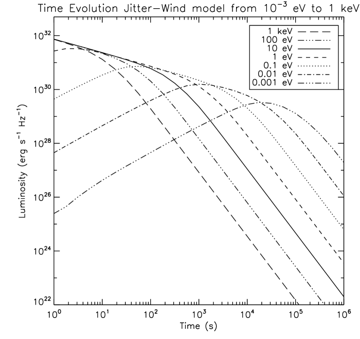
Figure 6: Comparison of light curves for jitter-wind model at different energies. The transition time between the luminosity scaling as $t^{-1/2}$ and $t^{-(3p-1)/4}$ is dependent on frequency and gives the appearance of a chromatic break in a power-law decay light curve. The time of this break ranges from about $t=10$s to $t=10^{5}$s for the frequencies shown in the figure.

Figure 7: Comparison of light curves for jitter-wind model in the X-ray ($h\nu=1$ keV), visible ($\lambda=575$ nm) and radio ($\nu=24.2$ GHz) bands, observed from $t=60$s to $t=10^{5}$s. The x-ray light curve is a single powerlaw decay, the visible is a broken powerlaw and the radio, in the optically thick regime, is a powerlaw increase.

References

- [1] Beloborodov A. M., 2005, ApJ, 627, 346
- [(Blandford & McKee 1976] Blandford R. D., & McKee C., F. 1976, Physics of Fluids, 19, 1130
- [2] Blustin A. J., et al., 2006, ApJ, 637, 901
- [3] Chang P., Spitkovsky A., Arons J., 2008, ApJ, 674, 378
- [(Chevalier & Li 2000] Chevalier R., & Li Z., 2000, ApJ 536, 212
- [4] Dai X., Halpern J. P., Morgan N. D., Armstrong E., Mirabal N., Haislip J. B., Reichart D. E., Stanek K. Z., 2007, ApJ, 658, 509
- [(Fleishman 2006)] Fleishman G., 2006a, ApJ, 638, 348
- [5] Fleishman G. D., 2006b, MNRAS, 365, L11
- [(Frederiksen et al. 2004)] Frederiksen J., Hededal C., Haugbølle T. & Nordlund Å., 2004, ApJ, 608, L13
- [6] Ghisellini G., Ghirlanda G., Nava L., Firmani C., 2007, ApJ, 658, L75
- [(Granot, Piran, and Sari (a) 1999)] Granot J., Piran T., & Sari R., 1999a, ApJ, 513, 679
- [Granot, Piran, and Sari (b) 1999] Granot J., Piran T., & Sari R., 1999b, ApJ, 527, 236
- [7] Huang K. Y., et al., 2007, ApJ, 654, L25
- [8] Liang E.-W., Zhang B.-B., Zhang B., 2007, ApJ, 670, 565
- [(Medvedev & Loeb 1999)] Medvedev M. V., & Loeb A., 1999, ApJ, 526, 697
- [(Medvedev 2000)] Medvedev M. V., 2000, ApJ, 540, 704
- [(Medvedev 2005)] Medvedev M. V., Fiore M., Fonseca R., Silva L. O., & Mori W., 2005, ApJ, 618, L75
- [(Medvedev 2006)] Medvedev M. V., 2006, ApJ, 637, 869
- [9] Medvedev M. V., Lazzati D., Morsony B. C., Workman J. C., 2007, ApJ, 666, 339
- [10] Meszaros P., & Rees M. J., 1997, ApJ, 476, 232
- [11] Nishikawa K.-I., Hardee P., Richardson G., Preece R., Sol H., Fishman G. J., 2003, ApJ, 595, 555
- [12] Nousek J. A., et al., 2006, ApJ, 642, 389
- [13] Panaitescu A., & Kumar P., 2001, ApJ, 554, 667
- [14] Panaitescu A., 2008, MNRAS, 383, 1143
- [15] Piran T., 1999, PhR, 314, 575
- [16] Rossi E., Rees M. J., 2003, MNRAS, 339, 881
- [(Rybicki & Lightman 1979)] Rybicki G. B., & Lightman A. P., 1979, Radiative Processes in Astrophysics. John Wiley & Sons, Inc., New York, New York
- [17] Sari R., Piran T., & Narayan R., 1998, ApJ, 497, L17
- [18] Silva L. O., Fonseca R. A., Tonge J. W., Dawson J. M., Mori W. B., Medvedev M. V., 2003, ApJ, 596, L121
- [19] Spitkovsky A., 2008, ApJ, 673, L39
- [20] Troja E., et al., 2007, ApJ, 665, 599
- [21] Uhm Z. L., Beloborodov A. M., 2007, ApJ, 665, L93
- [(Weibel 1959)] Weibel E. S., 1959, Phys. Rev. Lett., 2, 83
- [22] Wijers R. A. M. J., Rees M. J., Meszaros P., 1997, MNRAS, 288, L51
- [23] Workman J. C., Morsony B. J., Lazzati D., Medvedev M. V., 2008, MNRAS, 386, 199
- [24] Yost S. A., Harrison F. A., Sari R., Frail D. A., 2003, ApJ, 597, 459
- [(Zhang & Mészáros 2004)] Zhang B. & Mészáros P., 2004, International Journal of Modern Physics, 19, 2385