A flexible Bayesian method for adaptive measurement in psychophysics

Abstract

In psychophysical experiments time and the limited goodwill of participants is usually a major constraint. This has been the main motivation behind the early development of adaptive methods for the measurements of psychometric thresholds. More recently methods have been developed to measure whole psychometric functions in an adaptive way. Here we describe a Bayesian method to measure adaptively any aspect of a psychophysical function, taking inspiration from Kontsevich and Tyler’s (1999) optimal Bayesian measurement method. Our method is implemented in a complete and easy-to-use MATLAB package.

1 Motivation

Over the years a large number of methods have been developed with the goal to obtain the most information about an observer’s behaviour in a limited amount of time. They range from simple empirical schemes such as the staircase, to more elaborate mechanisms with better theoretical foundations, such as the QUEST or ZEST methods (Watson & Pelli,, 1983; King-Smith et al.,, 1994). Some only estimate the threshold, while others aim to provide information about the slope of the psychometric function as well (Kontsevich & Tyler,, 1999; Kujala & Lukka,, 2006).

Here we build on the latter to provide a very general framework for adaptive measurement and fitting of psychometric functions. We provide the option of focusing on a just one aspect of a psychometric function (for example, threshold or slope alone), or on the whole psychometric function. By using the framework of Bayesian inference, we provide theoretically well-founded methods for estimating the parameters and obtaining maximal information about them. An additional concern has been with the development of fast algorithms so that waiting time between trials could be minimised. We provide an easy-to-use software package in MATLAB for researchers without the time, the required technical background, or the inclination to implement our algorithms.

2 Description of the method

2.1 General framework

A psychometric function links the stimulus level (for example, contrast or signal-to-noise ratio) to a probability of response (often, the probability of a correct response). It can be defined by three parameters: one for the position along the stimulus level axis, one for the slope, and one for the lapse rate. The effects of the three are illustrated on figure 3. Thresholds are defined in the following way: first pick a performance level, for example 75%. Then the corresponding threshold is given by the inverse of the psychometric function, ie, it is the stimulus level such that the probability of response is 0.75.

The aim of a acquiring responses from an observer is to estimate some feature of the psychometric function, either its three parameters, or just its threshold or slope. The non-adaptive way to do this is for the experimenter is to spend some time in a dark room playing around with the stimulus and then choosing within a range a number of stimulus values they think appropriate to measure observer’s performance. This is known as the method of constant stimuli. The usual result is that due to variability between observers, and due also to the fact that the experimenter, having spent countless hours doing the task, will overestimate everybody else’s performance, thinking that 1% contrast should be easy enough for anyone. The method of constant stimuli thus leads to very wasteful data collection, with observers being tested at chance performance, or close to 100%. In the worst-case scenario, none of the datapoints are actually informative.

Despite this flaw, the method of constant stimuli enjoys the considerable resilience of a gold standard, notably because it results in fits that are easy to evaluate visually - but this is sometimes misleading, as we explain in section 2.9.7 below. The general class of alternatives to the method of constant stimuli is known in psychophysics as adaptive methods, and in other circles as active learning (Cohn et al.,, 1995). Adaptive methods take advantage of the intuitive idea that if an observer has already answered 10 out of 10 times correctly at a given level, then there isn’t much point in further interrogation.

In Bayesian adaptive methods, the measurement process is viewed as the step-by-step update of a probability distribution over the object of interest. Imagine we want to measure the 75% threshold: we start out by expressing our prior information about potential thresholds as a prior distribution. Just as in the case of the method of constant stimuli, we use the information acquired in the hours spent fiddling around and exploiting next-door colleagues to get some idea of what would be a range of realistic thresholds for other observers. This information will be udpated every time we collect a response from the observer: we update our beliefs according to whatever data we get. How exactly we need to update our beliefs is given by Bayes’ theorem. The process is illustrated in figure 1 and 2.

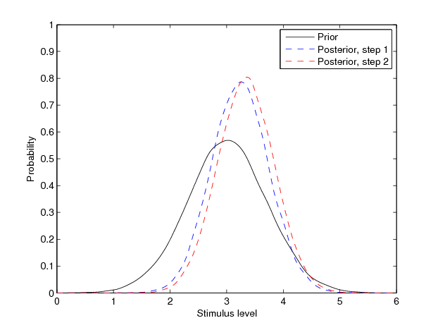
Figure 1: An illustration of Bayesian belief updating. We start out with a prior for the 75% threshold centered around 3 (black solid curve). On the first trial, we test the observer at stimulus level 6 and get an incorrect response. We update our beliefs according to Bayes’ theorem, yielding the first posterior distribution (blue dashed curve). The distribution agrees with intuitive reasoning: an incorrect response at level 6 would be unlikely if the real threshold were below 3, but more likely if it were above. On the 2d trial, the posterior from our first trial becomes our prior, and we measure a correct response at level 3, which is relatively likely under most threshold values between 2 and 4, and the posterior probability (red dashed curve) is changed only slightly. Notice how the uncertainty decreases over time, first fast, then more slowly. This is a general feature of Bayesian updating.

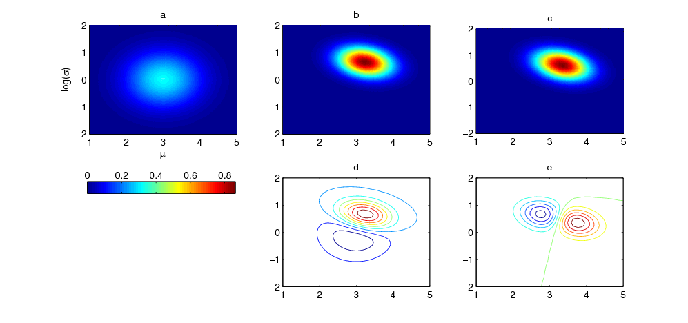
Figure 2: For the same data illustrated in figure 1, we show the Bayesian update in $\mu,\log\sigma$ space (see 2.2). a. Marginal prior over $\mu,\log\sigma$ b. Posterior after first trial c. Posterior after 2d trial. d. Difference between prior and first posterior e. Difference between second and first posterior. The updates are obtained via the Laplace approximation.

The uncertainty that remains about the threshold (or about any other set of parameters) is given by the entropy of the distribution. A distribution that has a single peak - indicating that we are extremely sure about the value of our parameter - will have minimum entropy, while a flat distribution - indicating complete lack of confidence - has maximum entropy. A decrease in entropy, then, is equivalent to an increase in confidence. At each step we ask: what is the stimulus level so that the confidence will increase maximally on average? Obviously if we know that the probability that the observer’s threshold is over 20% is 0.01, then there is no point in picking a stimulus level in the vicinity of 20%. The right stimulus level is given by a minimum in a cost function, which can be computed by the algorithms we detail below.

2.2 Functional form for the psychometric function

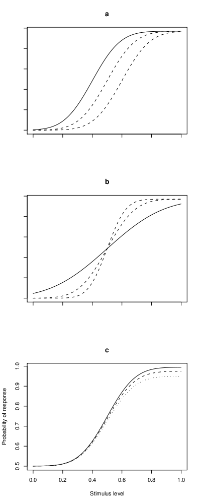
Figure 3: Effects of varying the parameters of the psychometric function. a. Increasing location, $\mu$ b. Increasing inverse slope $\sigma$ c. Increasing lapse rate $\lambda$

For psychometric functions in forced-choice experiments we use the following form:

$$\Psi(x;\mu,\sigma,\lambda)=(1-\lambda)\left(\gamma+(1-\gamma)\Phi(x;\mu,\sigma)\right)+\lambda\gamma$$ (1)

• x is the stimulus level

• $\mu$ and $\sigma$ describe the placement and slope of the psychometric function

• $\gamma$, a constant, is the chance rate. In 2AFC designs, $\gamma$ is set to 0.5.

• $\Phi(x;\mu,\sigma)$ is the cumulated Gaussian function. This choice of shape is on aesthetic grounds, choosing for example a logistic shape makes little to no difference in practice.

• Following the recommendations in Wichmann & Hill, 2001a ; Wichmann & Hill, 2001b we include a lapse term, $\lambda$. Here we assume that on every trial, the observer either lapses and makes a random choice (with probability of success $\gamma$) or behaves in a stimulus-dependent manner, with probability of success $\gamma+(1-\gamma)\Phi(x;\mu,\sigma)$. Including a lapse term is useful in order to insure robustness against random errors at high stimulus levels.

One can measure psychometric functions with different goals in mind. If the psychometric function is the independent variable in an experiment, one will wish to know its parameters $\theta=(\mu,\sigma,\lambda)$ as well as possible, using as few datapoints as possible. This is the aim of Kontsevich and Tyler’s original method. In another scenario, one wishes only to measure thresholds, for example to set the stimulus level in an experiment so that the difficulty is more or less the same for all observers, or simply because the threshold provides a useful summary of performance. Sometimes one may want to know more than just one threshold, for example both the $.73$ and the $.65$ thresholds could be of interest: we show in section 5.3 that this reduces to the $\Psi$ method solution.

2.3 The $\psi$ method

2.3.1 Description

The $\Psi$ method we describe here was first developed by Kontsevich & Tyler, (1999) and improved on by Kujala & Lukka, (2006). We frame the problem in Bayesian terms: our knowledge of the parameters of the psychometric function is described by a probability distribution over the parameters $\theta$. We start out with prior beliefs about $\theta$, descriped by a prior pdf $p_{0}(\theta)$, and at each step we collect data $y_{t}=(x_{t,}r_{t})$ where $r_{t}$ is the response and $x_{t}$ the stimulus level. We then update our beliefs according to Bayes’ theorem. We define $\mathbf{y_{t}}=(y_{1},y_{2},...,y_{t})$

$$p_{t}(\theta|\mathbf{y_{t}})=\frac{p(r_{t}|\theta)p_{t-1}\left(\theta|\mathbf{y_{t-1}}\right)}{p(\mathbf{y_{t})}}$$

From now on when not required for clarity we will drop the dependency of $\theta$ on $\mathbf{y}$ and simply write $p_{t}(\theta)$ for our posterior over $\theta$ at time $t$.

At any point in time, our uncertainty over the real value of the parameters can be summarised by the entropy of the posterior distribution:

$$H_{t}(\theta)=-\int p_{t}(\theta)\ln p_{t}(\theta)d\theta$$

The goal of the adaptive procedure must be to find the optimal stimulus placement so that the entropy is as low as possible when we are done collecting data. The optimal way of doing that would be to find at each time step the stimulus level that minimises expected entropy over all the remaining steps (Pelli,, 1987). This is computationally intractable and Nontsevick and Tyler’s $\Psi$ method only minimises the expected entropy over the next step, ie. it finds a $x_{t+1}$such that:

$$E_{r_{t+1}}\left(H_{t+1}(\theta)\right)$$

is minimised. Here $E_{r_{t+1}}$denotes the expectation over the unknown response $r_{t+1}$, given a stimulus level of $x_{t+1}$.

Intuitively, the $\Psi$method finds a stimulus level such that the observer’s response will have maximum effect (in expectation) on our beliefs. For example, if we know from our posterior on $\theta$ that the observer will be very close to 100% correct at a given stimulus level, then there is little point in placing the next trial at that level because the response is unlikely to teach us something new.

2.3.2 Computational issues

Computation of the posterior distribution

A number of computational issues arise in applying the $\Psi$ method. First, there is no closed form for the posterior $p_{t}(\theta)$, whatever the choice of prior, which makes it difficult to compute. Kontsevich & Tyler choose to discretise the parameter space, which leads to a difficult trade-off between precision and computation time and to many problems when parameter values lie near the boundaries. In their extension to the $\Psi$ method, Kujalla & Lucca use particle filtering to represent and update the posterior. Here we use a Laplace approximation (Mackay,, 2002), which is computationally very cheap and quite accurate for the right choice of parameterisation (see below). Given an unnormalised density $P(\theta)\propto p(\mathbf{y}|\theta)p(\theta)$, we find its mode $\theta^{*}$and approximate $P$ with $Q(\theta)$ a Gaussian centred on $\theta^{*}$. The covariance matrix of the Gaussian is given by the inverse of the Hessian of $\log Q$ at the mode. The approximation is accurate if $P(\theta)$ is unimodal and roughly symmetrical around its principal axes.

To improve the approximation should the need be felt, we provide the option of using importance resampling (Gelman et al.,, 2003). In importance resampling, $n$ samples $\{q\}$ from the approximating density $Q(\theta)$ are drawn. Each is given a weight:

$$w_{i}=\frac{P(q_{i})}{nQ(q_{i})}$$

We then draw $k<n$ samples without replacement from $\{q_{i}\}$ with probability $w_{i}$. In general this leads to an improvement in the approximation of the posterior density, because points that have low probability under $P(\theta)$ are less likely to be resampled.

Computation of the cost function

In Kontsevich and Tyler’s (1999) original formulation, the cost function for stimulus level is computed using algorithm 1. The cost function is computed over a predefined, discrete set of stimulus values and the best stimulus value is chosen. The algorithm is rather slow because it must compute a posterior distribution twice for each stimulus value. Kujalla & Lucca give a way of using a Fourier transform to reduce computational complexity.

Algorithm 1 Computing the K&T cost function, original algorithm

For each stimulus level $x_{t+1}$

1. Compute the probability of a correct response: $p_{t}(r_{t+1}=1|x_{t+1})=\sum_{\theta}p_{t}(\theta_{i})\Psi(x;\theta)$

2. For $r_{t+1}=$ 0 and 1: compute a posterior $p(\theta|r_{t+1},x_{t+1},\mathbf{y})$ and its entropy $H(r_{t+1}|x_{t+1})$

3. Compute $c(x_{t+1})=p_{t}(r_{t+1}=1|x_{t+1})H(r_{t+1}=1|x_{t+1})+p_{t}(r_{t+1}=0|x_{t+1})H(r_{t+1}=0|x_{t+1})$

More usefully to us, they have devised a reformulation of the cost function that enables fast computation when samples from the posterior are available. At each time step, $\theta$ is a continuous random variable with density given by $p_{t}(\theta)$. $r_{t+1}$, the observer’s next response, is a Bernoulli variable, whose probability of success $\pi_{t}(x_{t+1})$depends on the stimulus level. Minimising the $\Psi$ cost function is equivalent to finding the $x_{t+1}$ that maximises the mutual information between the response $r_{t+1}$ and $\theta$. The mutual information is symmetrical, thus:

$$I(r_{t+1},\theta)=H(\theta)-H(\theta|r_{t+1})=H(x_{t+1})-H(r_{t+1}|\theta)$$ (2)

The latter expression can be expanded as:

$$h\left(\pi_{t}(r_{t+1})\right)-\int p_{t}(\theta)h\left(\Psi(x_{t+1};\theta)\right)d\theta=h\left(\int p_{t}(\theta)\Psi(x_{t+1};\theta)d\theta\right)-\int p_{t}(\theta)h(\Psi(x_{t+1};\theta)d\theta$$

$h(\pi)$ is the entropy function for a Bernoulli variable $h(\pi)=-\pi\ln\pi-(1-\pi)\ln(1-\pi)$.

Given n samples $\{q_{i}\}$from the posterior or its approximation, an estimate of the cost function $c_{\Psi}$ is given by:

$$c_{\Psi}(x_{t+1})\approx h\left(n^{-1}\sum_{i=0}^{n}\Psi(x_{t+1},q_{i})\right)+n^{-1}\sum_{i=0}^{n}h\left(\Psi(x_{t+1},q_{i})\right)$$ (3)

The cost function can be computed with cost $\mathcal{O}(n)$.

2.3.3 Optimisation of the cost function

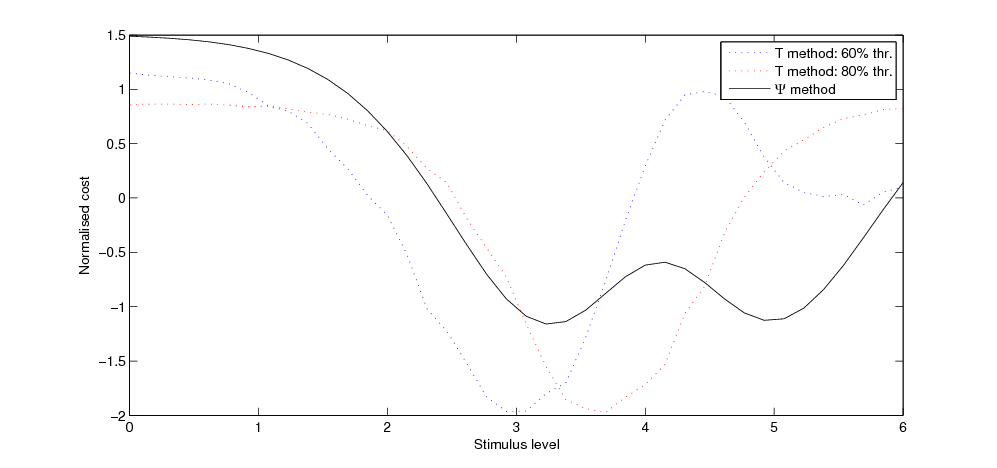
Figure 4: We simulate 100 trials of an adaptive run, and plot the different cost functions giving the best placement for the next trial according to different criteria. In the case of the cost functions computed using the $T$ method, we plot the estimates obtained using $6\times 10^{4}$ samples. The noisy nature of the estimates are still visible in the kinks of what would be otherwise smooth functions. Only one function is convex over the range illustrated here, see text for solutions to that problem.

The $\Psi$ cost function is in general not convex, and we have found empirically that in some cases it exhibits two local minima, see figure 4. To find the global minima several strategies can be used, including:

1. Sampling the function over a fixed grid, and starting a descent algorithm from the best point.

2. Using a descent algorithm with random restarts

The whole process is summed up in algorithm 2.

Algorithm 2 The $\Psi$ algorithm, fast version

At each time step t:

1. Find the maximum of the log posterior $p_{t}(\theta|\mathbf{y})$

2. Sample from the Laplace approximation to the log-posterior $p_{t}(\theta|\mathbf{y})$.

3. Find a minimum of the cost function $c_{\Psi}(x_{t+1})$, estimated from the posterior samples and equation (3).

4. Obtain observer response at stimulus level $x_{t+1}$.

2.4 Adaptive measurement for one attribute only: the $T$ method

Often when measuring psychophysical performance only one attribute is of interest: eg., the threshold, slope or range. The $T$ method takes inspiration from methods such as ZEST (King-Smith et al.,, 1994) and the $\Psi$ method described above, and provides an adaptive measurement algorithm for such cases. We describe the algorithm in detail for the case of measuring a threshold, the other two cases are similar. It is possible to generalise the algorithm to handle any function of the parameters into the real line, we show how below.

2.4.1 One threshold

A posteriori probability over a threshold

As we note above, quite often, the quantity of interest is the threshold, defined as the stimulus level such that the probability of a correct response is equal to $\alpha$. If the parameters $\theta^{*}$ are known, then the threshold $\tau_{\alpha}$ is expressed as:

$$\tau_{\alpha}=\{x:\Psi(x;\theta^{*})=\alpha\}$$

For a given parameter vector $\theta^{*}$ there is only one $x$ that satisfies this equation: $\Psi(x;\theta^{*})$ has an inverse, $\Psi^{-1}(\alpha;\theta^{*})$.

However, we have an uncertainty over $\theta$ that translates into an uncertainty over $\tau$. The posterior distribution over $\tau$ is given by:

$$p(\tau_{\alpha}|\mathbf{y})=\intop_{\theta}\delta\left(\Psi(\tau_{\alpha};\theta)=\alpha\right)p(\theta|\mathbf{y})d\theta$$

This is difficult to compute directly because for a given $\tau$ there are many $\theta$ such that $\Psi(\tau_{\alpha};\theta)=\alpha$ - we would need to integrate along a curve in $\mathbb{R}^{3}$. Fortunately, given samples from the posterior over $\theta$, it is easy to sample from $p(\tau_{\alpha}|\mathbf{y})$. We simply run the samples through $\Psi^{-1}$:

$$\Psi^{-1}(\alpha;q)\sim p(\tau_{\alpha}|\mathbf{y})\,\textrm{if}\,q\sim p(\theta|\mathbf{y})$$

Cost function for one threshold

Just as in the case of the $\Psi$-method outlined above, we want to maximise the quantity of information we gain at each step about the threshold $\tau$. Here again we proceed by choosing the $x_{t+1}$that maximises $I(r_{t+1},\tau)$, the mutual information between $r_{t+1}$ and the quantity of interest, $\tau$. There are a number of ways to compute that mutual information, but a fast method is to sample from the joint probability $p(r_{t+1},\tau)$, from the marginals $p(r_{t+1})$ and $p(\tau)$ and to estimate the mutual information from the samples.

We explained above how to sample from $p(\tau)$. $p(r_{t+1})$ is a Bernoulli random variable with probability of success $\int p_{t}(\theta)\Psi(x_{t+1};\theta)d\theta$. Sampling from the joint distribution is achieved by getting $\{q_{i}\}$ samples from $p(\theta|y)$. Then a sample pair from the joint distribution is obtained through:

$$\Psi^{-1}(\alpha;q_{i})$$

for the threshold and by simulating a Bernoulli variable with probability of success $\Psi(x_{t+1},q_{i})$ for the response.

Estimating the mutual information from samples is a whole topic in itself. Recall that the mutual information between two discrete random variables $X,Y$ is given by (Cover & Thomas,, 2006):

$$I(X,Y)=\sum_{X,Y}p(X,Y)\log\frac{p(X,Y)}{p(X)p(Y)}$$ (4)

One way to obtain an estimate of the mutual information between two continuous variables, or between one continuous and one discrete variable as is the case here, is to estimate their density by computing a histogram or using a kernel density estimator (Hastie et al.,, 2001). An estimate $\tilde{I}$ is obtained by plugging the numbers into equation 4, see 5.4 in the Appendix.

It turns out that here a faster method is available. Empirically, we observe that under the Laplace approximation $p(\tau|r_{t+1}=0)$ and $p(\tau|r_{t+1}=1)$ are often well approximated by Gaussians, especially when the performance wanted is around the mid-point (for example, 75% for a 2AFC experiment). Just as in equation 2, we write:

$$I(\tau,r_{t+1})=H(\tau)-H(\tau|r_{t+1})$$

Only the latter part of the right-hand side depends on the stimulus level through $r_{t+1}$. Therefore, to maximise the mutual information, we minimise :

$$H(\tau|r_{t+1})=-p(r_{t+1}=1)\int p(\tau|r_{t+1}=1)\log p(\tau|r_{t+1}=1)d\tau-p(r_{t+1}=0)\int p(\tau|r_{t+1}=0)\log p(\tau|r_{t+1}=0)d\tau$$ (5)

If we model the continous probability distribution functions in this expression as Gaussians, all we need to do is to compute the mean and variance of the samples from $p(\tau|r_{t+1}=0)$ and $p(\tau|r_{t+1}=1)$, the mutual information can then be computed by plugging the numbers into the expression for the entropy of a Gaussian, then into 5. Here again the time complexity of calculating the cost function at a single point is $\mathcal{0}(n)$, where $n$ is the number of samples. The number of samples required for a nearly-smooth approximation to the cost function is however much higher (e.g., 15,000), but in practice 5,000 samples yields good performance if a robust form of optimisation is used (section 2.8).

2.5 Adaptive estimation of width alone

The $\alpha$-width of a psychometric function is defined for the Yes/No case in Kuss et al., (2005) as:

$$w_{\alpha}=\Psi^{-1}(1-\alpha)-\Psi^{-1}(\alpha)$$

When $\alpha=10\%$, the width is the difference between the 90% and the 10% thresholds. This quantity is useful in describing the range of a psychometric function - contrary to slope measures, it is expressed in the same units as the stimulus. In NAFC experiments, an equivalent measure can be defined by:

$$w_{\alpha}=\Psi^{-1}(1-\alpha)-\Psi^{-1}(\gamma+\alpha)$$

For a 2AFC experiment ($\gamma=50\%$), and $\alpha=10\%$, $w_{10\%}$ is the difference between the 90% and the 60% thresholds.

To compute the mutual information between $w_{\alpha}$ and $r$, we proceed exactly as with thresholds, with the following modification: since $w_{\alpha}$ is bounded below by 0, the posterior distribution is assymetrical. A simple log-transformation renders it symmetrical, and we can apply our Gaussian method outlined above, or again use nonparametric density estimation.

2.6 Adaptive estimation of slope alone

For a cumulative Gaussian psychometric function such as we the one we use here the slope is inversely related to $\sigma$; therefore an appropriate measure of slope is

$$s=-\log\sigma=-\nu$$

Here again the same technique used for thresholds can be applied: a Gaussian approximation will do a very good job, but nonparametric estimation can be used as well.

2.7 Generalising to any function of the parameters

The threshold, slope and width as defined above are functions of the parameters $\theta=(\mu,\sigma,\lambda)$ into the real line. $\tau=\Psi^{-1}(\theta)$, $w_{\alpha}=\Psi^{-1}(1-\alpha)-\Psi^{-1}(\gamma+\alpha)$ and $s=-\log\sigma$. It is possible to generalise the algorithm to any function $f(\theta)$ into the real line, with $f$ defined according to the needs of the experiment. To maximise $I\left(r,f(\theta)\right)$ the algorithm given for thresholds applies directly, but care should be taken to check that the distributions $p\left(f(\theta)|r=0\right)$ and $p\left(f(\theta)|r=1\right)$ are well approximated by Gaussians. If not, then an appropriate transformation or non-parametric estimation should be used, see 5.4. Algorithm 3 presents the T method in its general form.

Algorithm 3 The T method

At each time step t, for a function $f(\theta)$ defining the quantity of interest.

1. Find the maximum of the log posterior $p_{t}(\theta|\mathbf{y})$

2. Get samples $\mathbf{q}_{\theta}$ from the Laplace approximation to the log-posterior $p_{t}(\theta|\mathbf{y})$,

3. For $k$ discrete levels of $x$: compute $\mathbf{q}_{f}=f(\mathbf{q}_{\theta})$, $\mathbf{q}_{r}=\Psi(x_{i};\mathbf{q}_{\theta})$, and sort the $\mathbf{q}_{f}$ according to $\mathbf{q}_{r}$ to obtain samples from $p_{t}\left(f(\theta)|r\right)$. Estimate $I\left(f(\theta)||r\right)$ using a parametric or non-parametric method.

4. Pick the point $x_{i}$ with the maximal estimated mutual information.

5. Obtain observer response at stimulus level $x_{t+1}$.

2.8 Optimising the cost function

Because it relies on random simulations, the $T$ cost function is noisy, unlike its $\Psi$ counterpart. Using a plain descent algorithm in this case is inappropriate, because the derivative information will be unreliable. A number of measures can be taken to cope with that problem. We highlight two.

The simplest is evaluation over a discrete grid, with an optional iterative refinement step around the minimum over the grid. One find the minimum over the grid, then expands another grid around the minimum, and iterates. Depending on the desired precision, the method may or may not be appropriate. If the possible stimulus levels are constrained to a discrete set in the first place (for example, contrast on a monitor), then simply evaluating the cost at every reasonable level makes sense.

Another option is to first evaluate the cost function over a discrete grid as above, to fit a smoothing model to the resulting points, and to optimise over the fitted model. A large number of techniques are available, including spline models(Hastie et al.,, 2001) and Gaussian Processes (Rasmussen & Williams,, 2005). A minor advantage of splines is that the minimum between each pair of knots can be computed analytically (and cheaply), although the primary cost is in the fitting. Interestingly, the optimal placement of points to find the minimum of a noisy function is itself an adaptive estimation problem that can be tackled via probabilistic models(Lizotte et al.,, 2007).

2.9 Statistical issues

2.9.1 Parameterisation, and choice of priors

We want to ensure that the posterior distribution is well-approximated by a Gaussian so that the Laplace method works well. This is difficult in the $\theta=(\mu,\sigma,\lambda)$ parameterisation because $\sigma\in]0,\infty[$ and $\lambda\in[0,1]$, and the parameter space is therefore bounded. We follow the recommendations in (Gelman et al.,, 2003) and use a reparameterisation, namely $\theta=(\mu,\nu,\eta)$, where:

$$\nu=\log(\sigma)$$

$$\eta=\textrm{logit}(\lambda)=\log\frac{\lambda}{(1-\lambda)}$$

This leaves us with parameters defined over $\mathcal{R}^{3}$, which is perfect for the Laplace approximation.

The natural choice of prior in that space is that of independent Gaussians, which can be made suitably vague by varying the standard deviation along each dimension:

$$p(\theta)=\mathcal{N}\left([m_{\mu},m_{\nu},m_{\eta}],[s_{\mu},s_{\nu},s_{\eta}]\mathbf{I}\right)$$

For $\eta$ fixed the the model is a generalised linear model, and in the limit $\eta\rightarrow-\inf$ the likelihood $p(\mathbf{y}|\theta)$ is a probit regression likelihood, and guaranteed to be log-concave (Paninski et al.,, 2004). In practice, to ensure that the posterior is uni-modal, the prior over $\eta$ should be made precise (ie, lapse-rates over 4 or 5% should be very improbable). That is not a major limitation, since, as Wichmann & Hill (; ) note, lapse rates above 5% make the measurement of psychometric functions very difficult and, should they occur, the experiment ought to be redesigned.

To get a “feel” for the prior, it is useful to display some draws from it, as in figure 5. The hyper-parameters can be adjusted until the researcher is confident that the prior contains realistic psychometric functions.

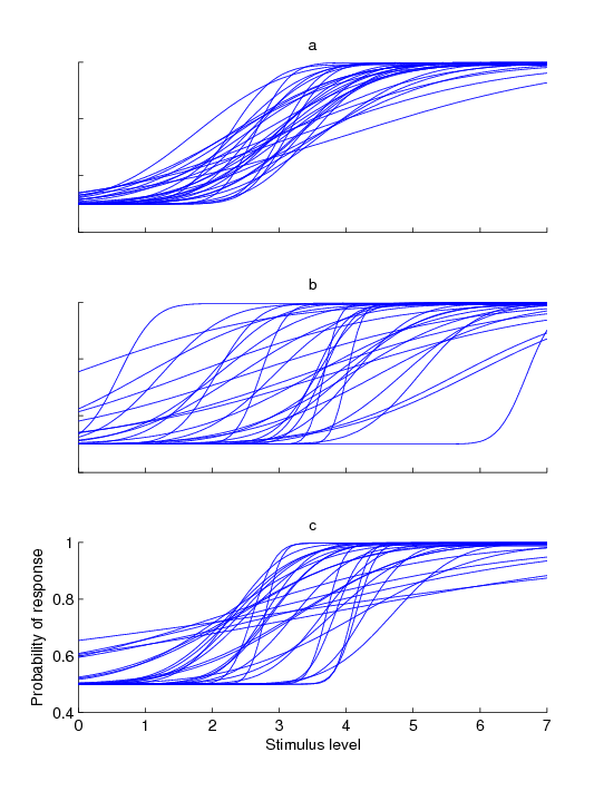
Figure 5: Adjusting the prior distribution. We display 30 psychometric functions, drawn from a Gaussian prior distribution. a) Tight prior over both $\mu$ and $\nu$ b) Looser prior over $\mu$ c) Looser prior over $\nu$

2.9.2 Posterior uncertainty

Confidence intervals over parameters

Approximate confidence intervals for $(\mu,\nu,\eta)$ or $(\mu,\sigma,\lambda)$ can be obtained from the empirical quantiles of the posterior distribution, or from the Hessian at the mode. Confidence intervals over thresholds $\mathbf{\tau}$ can be obtained in a similar way. The posterior often shows strong correlations between parameters, so in certain cases it might be worth taking a direct look at the probability volume, which can be done for instance via a slice representation. The same type of display can be used to make sure that the Laplace approximation is a good one (figure 6).

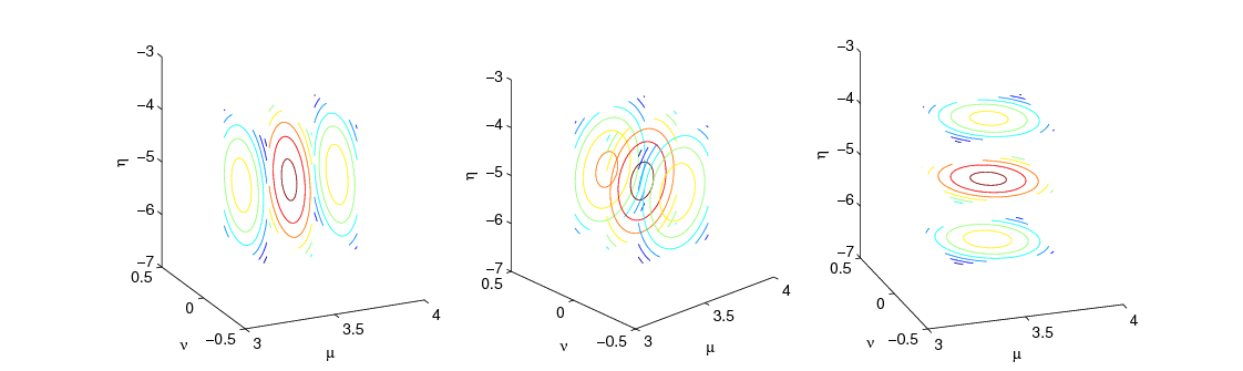
Figure 6: The posterior over parameters in a simulated experiment, after 200 trials. Slices across the three dimensions reveal nearly elliptical contours, showing that the Laplace approximation can be effective. The only aspect that is not well captured by a Laplace approximation is the slight sharpening of the contours in the direction of lower $\eta$ (the less an observer lapses, the more informative his or her responses are).

Posterior response distribution

As a useful display of posterior uncertainty, we also recommend plotting the posterior response distribution

$$p\left(\Psi(x)=q|\mathbf{y}\right)=p(\Psi^{-1}(q;x)|\mathbf{y})$$ (6)

where $\Psi^{-1}(q;x)$ is the $\theta$ such that $\Psi(x;\theta)=q$. In words, that distribution expresses “given the data y, what is the probability that the probability correct of the observer at stimulus level $x$ is $q$?”.

We plot the quantiles of that distribution for a simulated experiment in figure X, where color corresponds to quantile rank. Another useful visualisation is to display draws from the posterior, which can be compared with draws from the prior (figure X).

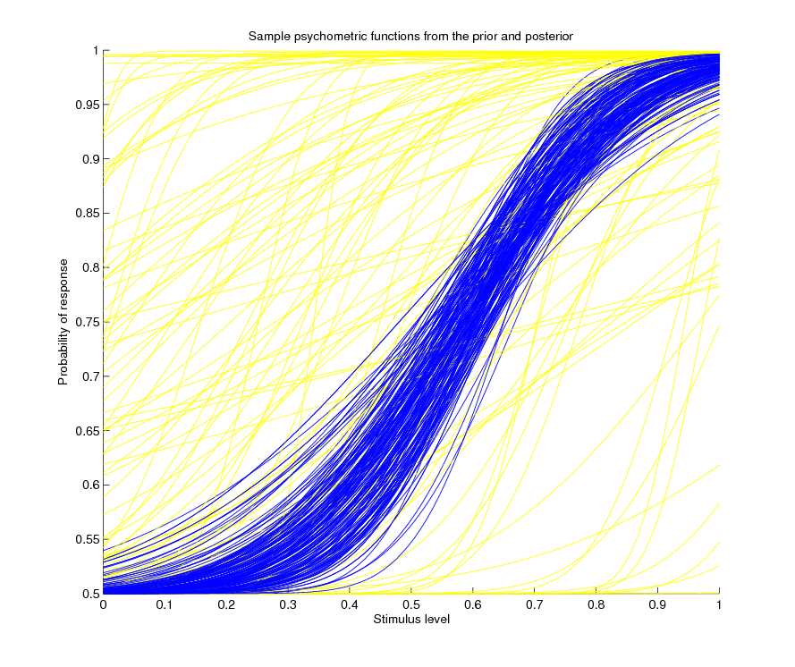
Figure 7: Comparing posterior to prior uncertainty. After a simulated experiment of 300 trials, samples from the posterior distribution (in blue) are plotted along with samples from the prior (in yellow).

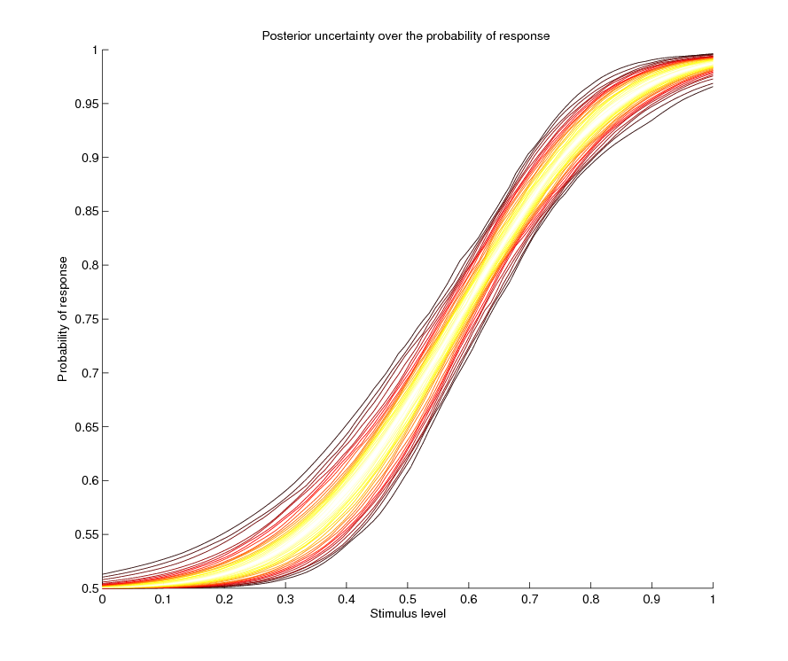
Figure 8: Posterior response uncertainty. With the same data as in figure (7), we plot the level lines of $p\left(\Psi(x)=q|\mathbf{y}\right)$ with line color corresponding to quantiles.

2.9.3 Stopping rules

Instead of stopping the procedure after a pre-set number of steps, the researcher may want a certain level of confidence to be reached. A simple solution is to interrupt the procedure after a certain entropy has been reached. The entropy can be estimated by the entropy of the Laplace approximation: recall that the covariance matrix is given by the inverse Hessian at the mode. We see from LABEL:eq:entG that a stopping rule can be established by setting a minimum level for $\det(\mathbf{G}^{-1})$, where $\mathbf{G}$ is the Hessian at the mode.

A more intuitive class of stopping rules is “don’t stop until we’re X% sure that a parameter is within certain limits”. This can be simply read off posterior samples. For example if the rule is: “don’t stop until we’re 95% sure that the threshold is above 1”, all one needs to do is to find out the proportion of posterior threshold samples that lie above 1.

2.9.4 Estimating response probability

The usual custom in psychophysics is to fit a psychometric function to the data, and to use the fitted values for predictions. If the probability of response at a given stimulus level is of interest then that is not the best strategy. To estimate that probability of response it makes more sense to average over values of the parameters:

$$p(r;x)=\int_{\theta}p(\theta|\mathbf{y})\Psi(x;\theta)d\theta$$

rather than use the estimated $\hat{\theta}$and compute $\hat{p}(r;x)=\Psi(x;\hat{\theta})$. Given large amounts of data the difference will be insignificant, but given small amounts it might not.

2.9.5 The estimates are biased!

Correct, if bias is understood in the statistical sense, ie for parameter $\theta$ and estimator $\hat{\theta}$ as $E(\hat{\theta}-\theta)$. If you have a prior that says that $\theta$ is more likely to be, say, 1, while the real theta is .8, then the estimator used here, the mean of the posterior distribution is going to be some compromise between what the data are saying (.8), and what the prior is saying. On the other hand, given the fact that $\theta$ is unknown, and whatever we know of it is contained in the prior and in the data, the mean of the posterior represents our best guess - choosing an unbiased estimator would imply disregarding the prior information, leading to far worse performance in practice.

2.9.6 How do I know my prior is correct? Can I avoid using one?

There are different aspects to that question. The first one is the question of how the use of a prior influences the final estimates. If the data are sufficient, and the prior is not too precise, the answer is not much at all. It is very easy to check for this: once the data have been collected, simply re-estimate the parameters of interest with a loosened prior. In the limit of high prior variance, the maximum a posteriori estimate tends to the maximum likelihood estimate, and in the limit of large data as well. When the data do not constrain the parameters very well, the maximum a posteriori estimate and the maximum likelihood estimate may be quite different. In that case, the maximum likelihood estimate can be clearly non-sensical, and prior constraints will help getting something sensible. What to do depends on what the data are needed for: if the adaptive procedure is used prior to an experiment to set levels appropriate to an observer’s performance, then good prior information can compensate to some extent for not-so-good data. If the adaptive procedure is used to collect the main data, then estimates that are not very robust to prior assumptions may be really bad news. Devising clever statistical procedures based on hierarchical models (Gelman et al.,, 2003) is a way of salvaging such data but running more subjects might be the simplest solution.

The second, potentially separate issue is the use of prior information for adaptive measurement. Such information is essential to avoid wasting trials testing observers on stupidly high or low stimulus intensity. Fortunately, this is quite easy to do. The software package we wrote includes a graphical utility for setting a prior that makes sense. As an experimenter, some simple considerations can help decide how to tune the parameters of the prior. For example, in a detection task, if an observer cannot detect the stimulus at 100% contrast, something must be going really wrong. Plotting prior proabibility of response, as in figure 9, helps modify the prior to take that fact into account. It is also safe to assume that if the overtrained experimenter can’t see the stimulus the subjects won’t be able to either. Again, it’s fairly easy to set the prior so that simple constraint is taken into account. Setting a prior on the slope is not too difficult either: do we believe observers can go from 50% correct to 95% correct in the space of a contrast increment? If yes, then prior samples should show that feature, if not then they should not (see figure 5).

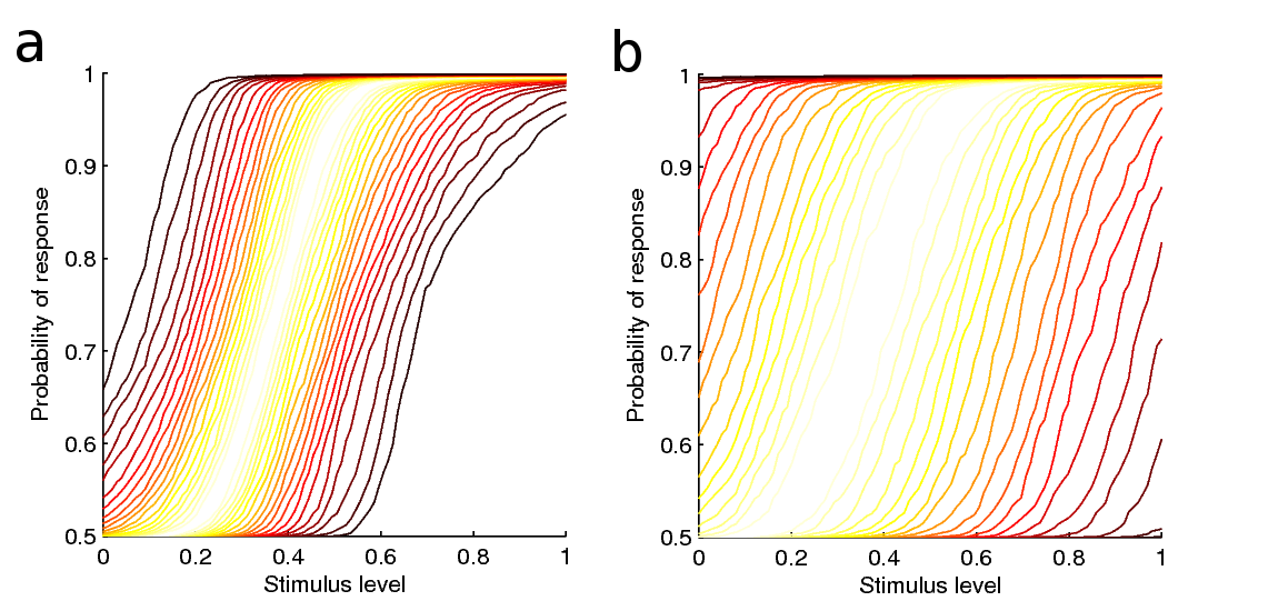
Figure 9: Adjusting the prior using the prior response probability. The level curves in the above figures are level lines of $p(\Psi(x))=\Psi(x;\theta)p(\theta)$ for a prior that is tight in $\mu$ (figure a) and one that is very wide (figure b). In the context of a detection experiment, suppose a stimulus level of 1 is the highest luminance that can be displayed. Clearly if the observer is still at chance for that level there is something wrong with the experiment or with the observer. Knowing that, the prior response probability of figure a is more appropriate than that of figure b.

2.9.7 I can’t check the fits by eye!

When using the method of constant stimuli, psychophysicists like to plot the measured proportion at each level along with the fit. The fit is then deemed to be good if it appears to go more or less through the datapoints.

One caveat is that psychometric functions are usually plotted on a probability scale because everyone likes a nice S-shape. This is unfortunately inappropriate for judging a fit because, unlike in least-squares regression, binomial error can’t be assessed from Euclidean distances in a plot on a probability scale. Predicting 50% and measuring 60% is not bad, predicting 90% and measuring 80% can be. The problem can be alleviated by plotting the psychometric function on a probit scale, which will make the psychometric function almost linear, and by providing sampling intervals for the fitted psychometric function. The sampling intervals answer the question: if the model is true, where would the central 95% of the measured values lie? This is given by the binomial distribution, is asymetrical and therefore does not map to the Euclidean metric we use to “eyeball” fits.

When running an adaptive experiment, we measure responses at many different points along the stimulus level axis, and we do it only once. It is not possible to plot the proportion of responses in this way, and therefore the familiar plot of the fitted psychometric function is impossible. Not all is lost, because there are alternatives.

A bad alternative is to bin together responses from nearby levels (this bad idea has nonetheless been used in several papers we won’t cite). This does not make any sense because we cannot, on the one hand, assume that the probability of response varies continuously with the stimulus level and then act as if it did not, by binning. Furthermore, there is no unique criterion to determine the size of the bins, and sizes could be hand-picked such as to make the fit look good or bad.

A simple alternative is to plot the responses as dashes along the stimulus level axis, as shown in figure X. This makes it possible to diagnose really bad fits (arising from a completely mistaken prior, either too flat or too peaked), and to assess whether the psychometric function has been properly sampled.

A more sophisticated option is to use posterior predictive checks (Gelman et al.,, 2003). The intuition behind the method is that models that fit well should give the observed data high probability under the posterior. The posterior predictive distribution is given by:

$$p(\mathbf{y^{*}}|\mathbf{y})=\int_{\theta}p(\mathbf{y^{*}}|\theta)p(\theta|\mathbf{y})d\theta$$

It represents the probability of getting data $\mathbf{y}^{*}$ when we’ve observed data y. It is easy to generate samples from that distribution given samples from the posterior $p(\theta|\mathbf{y})$ - see 2.4. Posterior predictive checks compare the actual, measured data from simulated datasets obtained from the posterior

One possible problem that could arise when estimating a psychometric function is when performance changes over time, for example due to drifts in attention levels. An example diagnostic plot is given in figure X. Here we simulate an observer whose psychometric function changes in the course of an experiment: the $\mu$ parameter is under a downward drift, $\mu(t)=3.5$, and the other parameters are set as in 3.1.

We plot level, trial, response triplets $(i,x_{i},r_{i})$ with stimulus level along the x axis, trial number (time) along the y axis, and the response, correct or incorrect, is color coded. The actual dataset is plotted in figure 10, and in figure 11, we plot simulated datasets from the predictive distribution. The lack of fit can be seen from the overprediction of correct responses in the late trials and the underprediction in the early trials.

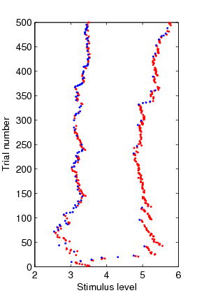
Figure 10: Posterior predictive checks. We plot the result of a simulated run of the $\Psi$ algorithm for an observer whose psychometric function changes over time (see text). Correct responses are plotted in red, incorrect responses in blue.

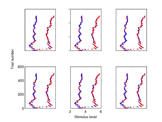
Figure 11: Simulated datasets from the posterior predictive distribution. Discrepancies with the observed data are visible.

3 Simulation results

We conducted an empirical evaluation of our software based on simulations. We report results on speed of convergence with respect to other sampling schemes, robustness to a misspecificed prior, and a comparison with the QUEST procedure.

3.1 The $\Psi$ method: speed of convergence

How well does the $\Psi$ method perform compared to other sampling schemes? We tested the following:

1. Uniform sampling from an interval. In this case the observer is tested at levels drawn uniformly from an interval. We test varied the spread of the interval, from wide (between 50.01% and 98.5% correct), medium (between 55% and 95% correct) to tight (the interval only covers values of the psychometric function between 70% correct and 85% correct).

2. Constant stimulus: we picked 6 stimulus levels for testing the observer. Here again we varied the spread of the levels: we took the same 3 intervals used for uniform sampling and divided them into 5 parts of equal length.

3. Our version of the $\Psi$ method.

We took the case of a 2AFC experiment. The lapse rate of the simulated observer was set to 2%. The simulated psychometric function is show in figure X, along with the sampling schemes we used. We varied the number of trials from 50 to 500, and took the mean a posteriori of $\mu$ and $\nu$ given the data as our estimates. We show the m.s.e. as a function of number of trials for the different conditions in figure X. We set the “true” parameters to $\mu=3.5$, $\nu=0.5$, with priors:

$$\mu\sim\mathcal{N}(3,\sqrt{0.5})$$

$$\nu\sim\mathcal{N}(0,\sqrt{0.5})$$

The results are shown on figure 12.

An important observation is that a tight interval around the threshold yields a good estimate of $\mu$ but a bad estimate of $\nu$, and vice-versa for a wide estimate. The $\Psi$ method seeks a compromise between the two, and achieves much better performance than the medium ’trade-off’ sampling scheme, as is evident from the figures.

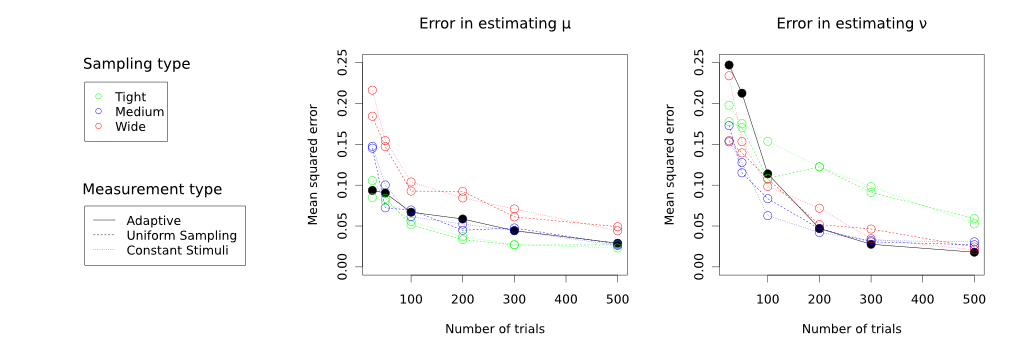
Figure 12: Comparison of measurement methods and sampling schemes. Mean squared error is plotted as a function of number of simulated trials (each datapoint represents an average over 150 simulated experiments) .

3.2 Robustness

In the paragraph above, the true values of the parameters are each one standard deviation away from the assumed prior mean. We’d like to know how the $\Psi$ method behaves when true values turn up to be very unlikely under the prior, ie. how robust it is to prior assumptions.

We repeat the experiment above, still setting $\mu=3.5$ and $\nu=0.5$, but starting with the following priors

1. $\mu\sim\mathcal{N}(3,\sqrt{0.5})$: true value less than one standard deviation away, precise prior

2. $\mu\sim\mathcal{N}(2,\sqrt{0.5})$ true value more than two standard deviations away, precise prior

3. $\mu\sim\mathcal{N}(3,1)$ true value 1.5 standard deviations away, vague prior

The results are plotted on figure 13. Prior (2) giving little prior probability to the true value starts off dramatically bad, but shows roughly exponential recovery. Prior (3) shows less bias and catches up with prior (2) quite fast. Bayesian asymptotics guarantee that as long as the prior gives non-null probability to the true value of the parameter, the maximum of the posterior will converge to the true value in the limit of large data. The lesson here is that vague priors are the prudent way to go if the circumstances allow. One way to check for large violations of prior assumptions during data analysis is to compare MAP and ML estimates to make sure there are no systematic discrepancies.

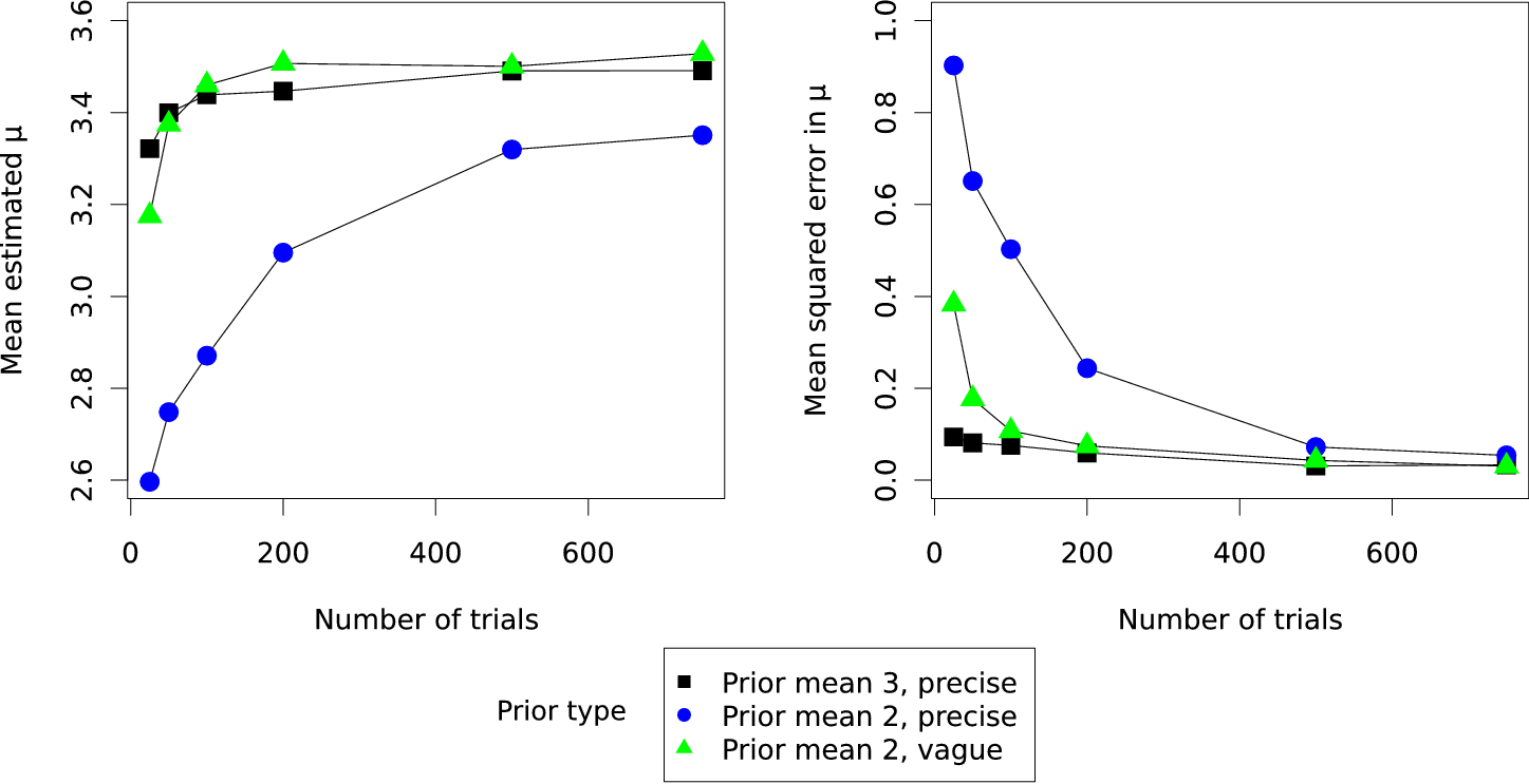
Figure 13: Experiments were simulated using three different types of priors. The mean estimate of $\mu$ and the associated mean square error are displayed as a function of the number of trials. Each datapoint represents an average over 150 simulated experiments.

3.3 T method versus QUEST

Although now a quarter of a century old, the QUEST algorithm remains a widely-used tool for the adaptive measurement of psychometric thresholds, one of the reasons being that it is available in a quality implementation in the popular package PsychToolbox (Brainard,, 1997; Pelli,, 1997). In this simulation we compare QUEST’s performance to that of the T method.

For the comparison to be fair, three issues had to be settled. The first issue is that QUEST assumes that the psychometric function has Weibull shape, whereas we assume it is a cumulated Gaussian. We account for that by simulating alternatively an observer with Weibull shape and an observer with Gaussian shape. We set the parameters for the Gaussian observer to $\mu=6,\nu=0.5$, and adjusted the parameters $\alpha,\beta$ of the Weibull observer so that the shape of the psychometric function was as close as possible, as measured by $L_{2}$ distance.

$$argmin_{\alpha,\beta}\int_{0}^{+\inf}\left(\Psi(x;\mu,\nu,\eta)-\Psi_{w}(x;\alpha,\beta,\eta)\right)^{2}dx$$ (7)

The Weibull psychometric function is a variant of 1:

$$\Psi_{w}(x;\mu,\sigma,\lambda)=(1-\lambda)\left(\gamma+(1-\gamma)w(x;\alpha,\beta)\right)+\lambda\gamma$$ (8)

$w(x;\alpha,\beta)=1-\exp\left(-\left(\frac{x}{\alpha}\right)^{\beta}\right)$ is the Weibull function. The integral 7 has no analytical form, so we used numerical integration and numerical optimisation. The result of the adjusment is displayed on figure 14. To keep things even half of the trials were run with the Weibull observer, and half without.

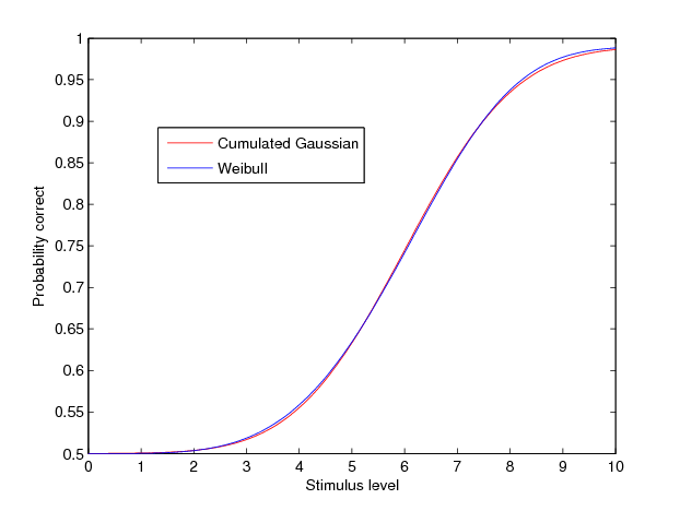
Figure 14: The psychometric function of the simulated Weibull observer was adjusted so as to match that of the cumulated Gaussian observer as closely as possible, as measured by $L_{2}$ distance. The resulting psychometric function is plotted in blue, with the target in red.

The second set of issues has to do with the prior assumptions embedded in the QUEST algorithms. We needed to ensure that the comparison was fair in terms of assumed prior knowledge, that QUEST did not know more a priori about the parameters than our method and vice-versa:

• QUEST asks the user to provide a “guess” for the threshold along with a prior variance. We therefore initialised QUEST with a guess and prior variance for the threshold corresponding to the mean and variance of $p(\tau|\mu,\nu,\eta)$, obtained by simulating from the prior for the T method and computing the threshold for each sample (as in section 2.4.1).

• QUEST assumes a known parameter$\beta$ in 8, but this parameter is never known exactly in practice. So QUEST’s $\beta$ value was set each time to a different, random, value to express the prior uncertainty in this parameter. Again, we sampled from the prior $p(\mu,\nu,\eta)$ and computed the best fitting $\alpha,\beta$ values by optimisation of 7 as explained above. $p(\log\beta|\mu,\nu,\eta)$ had a Gaussian distribution with mean 2.33 and standard deviation 0.77. Therefore, in every simulated QUEST experiment, we set $\log\beta$ to a random value from $\mathcal{N}(2.33,0.77)$.

• QUEST’s performance depends on a precision parameter. We increased the precision parameter until no further visible performance gain could be obtained. The performance of the T method can be increased by using more samples from the posterior, by refining the optimisation grid, by using non-parametric estimation, etc. We set the number of samples to 5000, the number of grid points to 45, and did not use non-parametric estimation. Those settings keep computing time to a reasonable 280ms per trial on the not-so-recent computer we used to run the tests.

We used the functions QuestQuantile to determine stimulus level and QuestMean for the final estimate. The results are shown on figure 15. The T method has a lead when the number of trials is low, but at 200 trials the methods yield essentially identical results. Although some marginal improvements could still be had in the T method by increasing the computational load, this leads us to think that in the case of estimating thresholds we are close to ceiling performance, unless we move to more sophisticated models than the psychometric function (e.g., models that take into account possible interdependencies between trial outcomes instead of assuming independence).

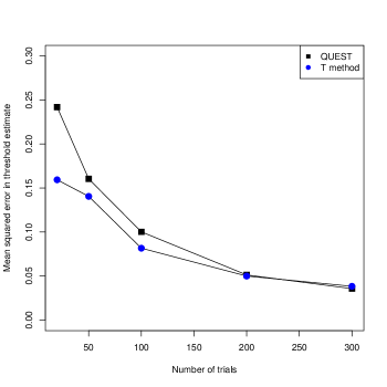
Figure 15: Comparison of QUEST and the T method. We plot the mean squared error in estimation of the 75% threshold (each datapoint represents an average over 100 simulated experiments).

4 Conclusion

Our framework can easily be extended to a range of related problems, such as the adaptive measurement of psychometric surfaces (probability of response as a function of more than one stimulus dimension), as in Kujala & Lukka, (2006). A more challenging extension and a direction for future work is to model-based adaptive measurement in psychophysics (Lesmes et al.,, 2006). The usual course of action in psychophysical experiments is to acquire some data first, and then to fit models to evaluate hypotheses. Using the techniques outlined here it is possible to select stimuli to minimise the uncertainty about model parameters, or even to select stimuli that help determine which model is more appropriate - an adaptive form of hypothesis testing. We are currently investigating an application to the Bayesian estimation of classification images.

5 Appendix

5.1 Bayesian inference for psychometric functions

5.1.1 Computing the posterior

The posterior over the parameters $\theta=(\mu,\nu,\eta)$ given the data is given by:

$$p(\theta|\mathbf{y})=\frac{p(\mathbf{y}|\theta)p(\theta)}{p(\mathbf{y})}$$

Where the likelihood is equal to:

$$p(\mathbf{y}|\theta)=p\left(\{\mathbf{r},\mathbf{x}\}|\theta\right)=\prod_{i=1}^{N}\left(r_{i}\Psi(x_{i},\theta)+(1-r_{i})(1-\Psi(x_{i},\theta))\right)$$

The posterior has no closed form solution, so an approximation must be used. Kuss et al., (2005) use reversible-jump Markov Chain Monte Carlo, but we found that the much simpler Laplace approximation works well enough for most purposes, given the appropriate parameterisation (section 2.9.1).

If something more precise is needed, the posterior is only three-dimensional so traditional numerical integration, while slow, is still tractable. We recommend integrating over a cubic region that includes most of the mass of the Laplace approximation, in case the Laplace approximation is much sharper than the actual density. The density is continuous and twice differentiable so traditional integration rules apply.

5.1.2 Integrating out the lapse rate

In many cases the lapse parameter $\eta=\textrm{logit}(\lambda)$ is a nuisance variable of no direct interest. The standard way of dealing with nuisance variables in Bayesian statistics is by “integrating out”:

$$p(\mu,\nu|\mathbf{y})=\int_{-\inf}^{+\inf}p(\mu,\nu,\eta|\mathbf{y})d\eta$$ (9)

Under the Laplace approximation, $p(\mu,\nu,\eta|\mathbf{y})$ is multivariate Gaussian and therefore so is $p(\mu,\nu|\mathbf{y})$, and the correlation matrix is unchanged (Rasmussen & Williams,, 2005). When working with samples from the posterior if $(\mu^{*},\nu^{*},\eta^{*})$ are samples from $p(\mu,\nu,\eta|\mathbf{y})$ then $(\mu^{*},\nu^{*})$ are samples from $p(\mu,\nu|\mathbf{y})$.

5.2 The psychometric function in Yes/No experiments

In Yes/No experiments the range of the psychometric function is $[0,1]$. We adopt the following functional form:

$$\Psi(x;\mu,\sigma,\lambda)=(1-\lambda)\Phi(x;\mu,\sigma)+\frac{\lambda}{2}$$ (10)

The parameters have the same interpretation as in the forced-choice case, see 2.2.

5.3 Reduction of the multiple-threshold case to the $\Psi$ method

Suppose that the researcher wishes to find appropriate stimulus levels to put the observer at 0.65, 0.75 and 0.85 performance. In other words, he or she needs to estimate a vector $\mathbf{\tau}$ of thresholds. In cases maximising the mutual information between $\mathbf{\tau}$ and the observer’s responses is equivalent to maximising the mutual information between $\theta$ and the observer’s responses (approximately for two thresholds, exactly for three and more). In other words, the $\Psi$ method is appropriate in this case.

This is quite easy to see: if we know $\theta$ then $\tau$ is known (the psychometric function defines unique thresholds). On the other hand, if we know that $\Psi(x_{1};\mu,\sigma,\lambda)=q_{1}$,$\Psi(x_{2};\mu,\sigma,\lambda)=q_{2}$,$\Psi(x_{3};\mu,\sigma,\lambda)=q_{3}$ (ie we know three thresholds), then we know $\theta=(\mu,\sigma,\lambda)$. Each known threshold fixes one parameter with respect to the others. Therefore there exists a one-to-one correspondence between $\theta$ and $\mathbf{\tau}$, so that in probabilistic terms, a density over $\theta$ is a transformation of a density over $\tau$, and vice versa. The mutual information is invariant to transformations of the variables, therefore $I(\mathbf{\theta},\mathbf{r})=I(\mathbf{\tau},\mathbf{r})$ and the $\Psi$ method applies.

In the case where $\tau$ is two-dimensional then the one-to-one correspondence does not exist, and:

$$p\left(\tau_{q_{1},q_{2}}=(x_{1},x_{2})\right)=\int_{\Theta}I_{\theta,\tau}p(\theta)d\theta$$

where $I_{\theta,\tau}$ is the indicator function of the solution set of $\left(\begin{array}[]{cc}\Psi(x_{1};\theta)&=q_{1}\\ \Psi(x_{2};\theta)&=q_{2}\end{array}\right)$, which contains all the $(\mu,\sigma,\lambda)$ triplets compatible with $q_{1},q_{2}$ thresholds being at $x_{1},x_{2}$. We’ll make a heuristic argument of why in this case the $\Psi$ method is still a good approximation.

Notice that $\lambda$, the lapse rate, affects thresholds very little within its normal range ($\lambda$ < 5%), especially for thresholds far from the extremes. So most of the uncertainty about the thresholds can be traced to uncertainty about $\mu$ and $\sigma$. Consequently, given two thresholds $\tau_{1}$ and $\tau_{2}$ known exactly, there is little uncertainty left in the estimation of $\mu$ and $\sigma$. This implies that having knowledge of $\theta$ and having knowledge of $\tau=(\tau_{1},\tau_{2})$ is almost the same thing, and gaining information about one is almost the same as gaining information about the other.

5.4 Nonparametric density estimation for the T method

The problem of estimating the mutual information between threshold (or width, or slope) and response hinges on the computation of the conditional densities of $p(\tau,r)$: $p(\tau|r)$, or, equivalently, $p(r|\tau)$. The first (a continuous density as a function of a binary variable) can be dealt with using non-parametric density estimation techniques, the second (a probability distribution over a binary variable as a function of a vector of continuous variables) can be dealt with using a multiplicity of techniques developed for logistic regression.

5.4.1 Kernel density estimation

Kernel density estimation is a natural extension of the well-honed technique of building histograms (Hastie et al.,, 2001). A histogram estimates a density $f_{X}$ by binning the data $\mathbf{X}=(\mathbf{x_{1},}\mathbf{x_{2},...,}\mathbf{x_{N})}$:

$$\hat{f_{X}}(x)=\frac{1}{N}\times B(x;\mathbf{X})$$

The function $B(x,\mathbf{X})=\sum_{i=1}^{N}I_{x}(x_{i})$, where $I_{x}$ is the indicator function for the bin that contains $x$, simply counts how many samples are in the same bin. Within that neighbourhood, all samples are given equal weighting, and without, all are discarded. This leads to non-smooth density estimates (as we’ve all noticed, histograms are blocky).

In kernel density estimation, to estimate $f_{X}(x)$, we weigh samples according to how far they are from $x$, with the weighting given by a kernel function. The kernel density estimate is given by

$$\hat{f}_{X,t}(x)=\frac{1}{Nt}\sum_{i=1}^{N}K(x,x_{i})$$

$K(x,x^{\prime})$ is a kernel function, generally a Gaussian (we promise this is the last occurence of the word Gaussian in this article). The smoothness parameter $t$ is estimated from the data. The kernel density estimator has better convergence properties than the histogram for smooth distributions. Once we have estimated $t$, the entropy estimate for the density $f_{X}(x)$ follows naturally

$$\hat{H}(f_{X})=-\int\hat{f}_{X,t}(x)\log\hat{f}_{X,t}(x)$$

This quantity can be computed numerically quite easily.

5.4.2 Advantages and shortcomings

The main advantage of the kernel density estimator is that it is non-parametric. The main problem here is that density estimation or non-parametric logistic regression occurs within an optimisation loop, so that time complexity is the major issue. If we require m evaluations of $\hat{f}_{X,t}$ to compute the entropy estimate based on n samples, a naive implementation would have $\mathcal{O}(mn)$ time complexity. A clever implementation based on the Fast Fourier Transform can bring that down to $\mathcal{O}(m\log n)$.

As a proof of concept, we have implemented support for Gray and Moore’s (Gray & Moore,, 2003) kernel density estimator, which uses a tree structure to speed up processing. Alternatively, kernel logistic regression is a candidate for modelling $p(r|\tau)$. Unfortunately, the computational cost is still severe enough to make it prohibitive on all but the most recent desktop computers. Future advances will no doubt make this practical.

References

- Brainard, (1997) Brainard, D. H. (1997). The psychophysics toolbox. Spat Vis, 10(4), 433–436.
- Cohn et al., (1995) Cohn, D. A., Ghahramani, Z., & Jordan, M. I. (1995). Active learning with statistical models. In G. Tesauro, D. Touretzky, & T. Leen (Eds.), Advances in Neural Information Processing Systems, volume 7 (pp. 705–712).: The MIT Press.
- Cover & Thomas, (2006) Cover, T. M. & Thomas, J. A. (2006). Elements of Information Theory 2nd Edition (Wiley Series in Telecommunications and Signal Processing). Wiley-Interscience.
- Gelman et al., (2003) Gelman, A., Carlin, J. B., Stern, H. S., & Rubin, D. B. (2003). Bayesian Data Analysis. Chapman & Hall.
- Gray & Moore, (2003) Gray, A. G. & Moore, A. W. (2003). Nonparametric density estimation: Toward computational tractability. In SIAM Data Mining.
- Hastie et al., (2001) Hastie, T., Tibshirani, R., & Friedman, J. H. (2001). The Elements of Statistical Learning. Springer.
- King-Smith et al., (1994) King-Smith, P. E., Grigsby, S. S., Vingrys, A. J., Benes, S. C., & Supowit, A. (1994). Efficient and unbiased modifications of the quest threshold method: theory, simulations, experimental evaluation and practical implementation. Vision Research, 34(7), 885–912.
- Kontsevich & Tyler, (1999) Kontsevich, L. L. & Tyler, C. W. (1999). Bayesian adaptive estimation of psychometric slope and threshold. Vision Res, 39(16), 2729–2737.
- Kujala & Lukka, (2006) Kujala, J. V. & Lukka, T. J. (2006). Bayesian adaptive estimation: The next dimension. Journal of Mathematical Psychology, 50(4), 369–389.
- Kuss et al., (2005) Kuss, M., Jäkel, F., & Wichmann, F. A. (2005). Bayesian inference for psychometric functions. Journal of Vision, 5(5), 478–492.
- Lesmes et al., (2006) Lesmes, L. A., Jeon, S. T., Lu, Z. L., & Dosher, B. A. (2006). Bayesian adaptive estimation of threshold versus contrast external noise functions: the quick tvc method. Vision Res, 46(19), 3160–3176.
- Lizotte et al., (2007) Lizotte, D., Wang, T., Bowling, M., & Schuurmans, D. (2007). Automatic gait optimization with gaussian process regression. In M. Veloso (Ed.), Proceedings of the Twentieth International Joint Conference on Artificial Intelligence.
- Mackay, (2002) Mackay, D. J. C. (2002). Information Theory, Inference & Learning Algorithms. Cambridge University Press.
- Paninski et al., (2004) Paninski, L., Pillow, J. W., & Simoncelli, E. P. (2004). Maximum likelihood estimation of a stochastic integrate-and-fire neural encoding model. Neural Comput, 16(12), 2533–2561.
- Pelli, (1987) Pelli, D. (1987). The ideal psychometric procedure. Investigative Ophthalmology and Visual Science (Supplement), 28, 366+.
- Pelli, (1997) Pelli, D. G. (1997). The videotoolbox software for visual psychophysics: transforming numbers into movies. Spat Vis, 10(4), 437–442.
- Rasmussen & Williams, (2005) Rasmussen, C. E. & Williams, C. K. I. (2005). Gaussian Processes for Machine Learning (Adaptive Computation and Machine Learning). The MIT Press.
- Watson & Pelli, (1983) Watson, A. B. & Pelli, D. G. (1983). Quest: a bayesian adaptive psychometric method. Percept Psychophys, 33(2), 113–120.
- (19) Wichmann, F. A. & Hill, N. J. (2001a). The psychometric function: I. fitting, sampling, and goodness of fit. Percept Psychophys, 63(8), 1293–1313.
- (20) Wichmann, F. A. & Hill, N. J. (2001b). The psychometric function: Ii. bootstrap-based confidence intervals and sampling. Percept Psychophys, 63(8), 1314–1329.