NT@UW-08-16
Understanding the Optical Potential in HBT Interferometry

Abstract

The validity of using a pion optical potential to incorporate the effects of final state interactions on HBT interferometry is investigated. We find that if the optical potential is real, the standard formalism is modified as previously described in the literature. However, if the optical potential is complex, a new term involving pion emission from eliminated states must be included. The size of such effects in previous work by Cramer and Miller is assessed.

I Introduction

The space-time structure of the “fireball” produced in the collision between two relativistically moving heavy ions can be investigated by measuring two-particle momentum correlations between pairs of identical bosons. The Bose-Einstein enhancement of the coincidence rate at small momentum differences depends on the space-time extent of the particle source. This method of investigation, called HBT interferometry, has been applied extensively in recent experiments at the Relativistic Heavy Ion Collider (RHIC) by the STAR and PHENIX collaborations. See the reviewsPratt:wm ; Wiedemann:1999qn ; Kolb:2003dz ; Lisa:2005dd .

The invariant ratio of the cross section for the production of two pions of momenta ${\bf p}_{1},{\bf p}_{2}$ to the product of single particle production cross sections is analyzed as the correlation function $C({\bf p}_{1},{\bf p}_{2})$. We define ${\bf q}$=${\bf p}_{1}$–${\bf p}_{2}$ and ${\bf K}$=$({\bf p}_{1}$+${\bf p}_{2})/2$, with ${\bf K}_{T}$ as the component perpendicular to the beam direction. (We focus on mid-rapidity data, where ${\bf K}={\bf K}_{T}$.) The correlation function can be parameterized for small ${\bf q}$ as $C({\bf q},{\bf K})-1\approx\lambda\exp{(-R_{O}^{2}q_{O}^{2}-R_{S}^{2}q_{S}^{2}-R_{L}^{2}q_{L}^{2})}\approx\lambda(1-R_{O}^{2}q_{O}^{2}-R_{S}^{2}q_{S}^{2}-R_{L}^{2}q_{L}^{2})\;(q_{i}R_{i}\ll 1),$ where $O,S,L$ represent directions parallel to ${\bf K}_{T}$, perpendicular to both ${\bf K}_{T}$ and the beam direction, and parallel to the beam direction BP-HBT . Early Rischke:1996em and recent Kolb:2003dz hydrodynamic calculations predicted that a fireball evolving through a quark-gluon-hadronic phase transition would emit pions over a long time period, causing a large ratio $R_{O}/R_{S}$. The puzzling experimental result that $R_{O}/R_{S}\approx 1$ Adler:2001zd is part of what has been called “the RHIC HBT puzzle” Heinz:2002un . Another part of the puzzle is that the measured radii depend strongly on the average momentum $K$, typically decreasing in size by about 50% over the measured range, showing that the radii are not simply a property of a static source. The medium at RHIC seems to be a very high density, strongly interacting plasma Gyulassy:2004zy , so that any pions made in its interior could be expected to interact strongly before emerging. Thus one expects that the influence of the interactions between the pion probe and the medium, as well as flow and other effects, must be taken into account when extracting the radii.

We studied the effects of including the pionic interactions in previous work Cramer:2004ih ; Miller:2005ji . Distorted waves, instead of plane waves, were used to represent the pion wave functions. The resulting formalism is called the Distorted Wave Emission Function (DWEF) formalism because the emission function used to describe the space-time extent of the emitting system is dressed by the final state interactions. We found that it is possible to simultaneously describe the measured HBT radii and pionic spectra by including the effects of pion-medium final state interactions obtained by solving the relevant relativistic wave equation. These interactions are so strongly attractive that the pions act as essentially massless objects inside the medium. The medium acts as if it is free of the chiral condensate that is the source of the pion mass, and therefore acts as a system with a restored chiral symmetry. Other solutions of the HBT puzzle have been proposed. See the review Lisa:2005dd .

Some theorists have questioned whether waves, produced by incoherent sources, unaffected by final state interactions, interfere with those that are affected by final state interactions. That this interference occurs was demonstrated at least as early as 1979 Gyulassy , again in the nineties Barz:1996gr ; Barz:1998ce ; hh ; th , and there have been two recent publications confirming that conclusion Kapusta:2005pt , Wong:2003dh . The former derive a general formula for the correlation function of two identical particles including multiple elastic scatterings in the medium in which the two particles are produced. Numerical results for the case of soft final state interactions are presented. Ref. Wong:2003dh includes the effects occurring when emitted particles undergo multiple scattering with medium particles. Using the Glauber theory of multiple scattering at high energies and the optical model at intermediate energies, it is found that multiple scattering leads to an absorption.

Despite this progress, several conceptual issues remain. These include understanding: the meaning of the imaginary part of the optical potential, the role of the energy dependence of the optical potential Pratt:2007pf , and the relationship between the sources producing the pions and the optical potential. Therefore, we find it worthwhile to re-investigate the effects of quantum mechanical treatments of final state interactions.

Our procedure is to repeat the derivation of Ref. BP-HBT using a simple Lagrangian. First, the original plane wave treatment is reproduced using our notation, Sect. II. Then the effects of a real optical potential are incorporated, Sect. III. The result is a re-derivation of of the DWEF formalism. However, a deeper understanding is needed to correctly account for the effects of a complex optical potential. This can only be incorporated using a coupled channels formalism, Sect. IV. We find that including the complete effects of an imaginary optical potential requires a modification to the DWEF formalism that is presently incalculable. However, the optical potential used in Cramer:2004ih ; Miller:2005ji was dominated by its real part. In particular, in Sect. V we find that setting the imaginary part optical potential to zero does not significantly change our description of the data. Sect. VI is reserved for a summary and discussion.

II The Pratt Formalism

The space-time extent of a source of pions can be inferred by measuring the pionic correlations known as the Hanbury Brown-Twiss effect HBT ; HBT1 . The correlation function function $C({\bf p},{\bf q})$ is defined to be

$$C({\bf p},{\bf q})\equiv{P({\bf p},{\bf q})\over P({\bf p})P({\bf q})},$$ (1)

where $P({\bf p}_{1},\cdots{\bf p}_{n})$ is the probability of observing pions of momentum ${\bf p}_{i}$ all in the same event. The identical nature of all pions of the same charge cause $C({\bf p},{\bf p})=2$. The width of the correlation function is related to the space-time extent of the source.

A state created by a random pion source $|\eta\rangle$ is described by Gyulassy

$$|\eta\rangle=\exp[\int d^{4}x\eta(x)\gamma(t)\hat{\psi}^{\dagger}(x)]|0\rangle=\exp[\int d^{3}pdt\eta({\bf p},t)\gamma(t)c^{\dagger}({\bf p})e^{-iE_{p}t}]|0\rangle,$$ (2)

where $\hat{\psi}^{\dagger}$ is the pion creation operator in the Heisenberg representation, $\gamma(t)$ is the random phase factor that takes the chaotic nature of the source into account, and $c^{\dagger}({\bf p})$ is the creation operator for a pion of momentum ${\bf p}$.. In particular, an average over collision events gives

$$\langle\gamma^{*}(t)\gamma(t^{\prime})\rangle=\delta(t-t^{\prime}),\;\langle\gamma^{*}(t_{1})\gamma^{*}(t_{2})\gamma(t_{3})\gamma(t_{4})\rangle=\delta(t_{1}-t_{3})\delta(t_{2}-t_{4})+\delta(t_{1}-t_{4})\delta(t_{2}-t_{3}).$$ (3)

We note that as written, the state $|\eta\rangle$ is not normalized to one. However, the normalization constant will divide out of the numerator and denominator of the correlation function. Therefore we do not make the normalization factor explicit here, but note that it enters when we calculate the pion spectrum.

For $\hat{\psi}$ and its time derivative to obey the Heisenberg commutation relation one has

$$\sqrt{E_{p}E_{p^{\prime}}}[c({\bf p}),c^{\dagger}({\bf p}^{\prime})]=\delta^{(3)}({\bf p}-{\bf p}^{\prime}).$$ (4)

Furthermore, we define

$$\eta({\bf p},t)\equiv\int d^{3}xe^{-i{\bf p}\cdot{\bf x}}\eta(x).$$ (5)

The state $|\eta\rangle$ is an eigenstate of the destruction operator in the Schroedinger representation, $c({\bf p})$:

$$c({\bf p})|\eta\rangle=\int dte^{iE_{p}t}{\eta({\bf p},t)\over E_{p}}\gamma(t)|\eta\rangle.$$ (6)

The correlation function is

$$C({\bf p},{\bf q})={\langle\eta|c^{\dagger}({\bf p})c^{\dagger}({\bf q})c({\bf q})c({\bf p})|\eta\rangle\over\langle\eta|c^{\dagger}({\bf p})c({\bf p})|\eta\rangle\langle\eta|c^{\dagger}({\bf q})c({\bf q})|\eta\rangle}.$$ (7)

The use of Eq. (3) and Eq. (6) in the numerator of Eq. (7) yields

$$\langle\eta|c^{\dagger}({\bf p})c^{\dagger}({\bf q})c({\bf q})c({\bf p})|\eta\rangle=\langle\eta|c^{\dagger}({\bf p})c({\bf p})|\eta\rangle\langle\eta|c^{\dagger}({\bf q})c({\bf q})|\eta\rangle+|\langle\eta|c^{\dagger}({\bf p})c({\bf q})|\eta\rangle|^{2}.$$ (8)

Furthermore

$$\langle\eta|c^{\dagger}({\bf p})c({\bf q})|\eta\rangle=\int dt\exp[-i(E_{p}-E_{q})t]{\eta^{*}({\bf p},t)\eta({\bf q},t)\over E_{p}E_{q}}.$$ (9)

The quantity $g(x,{\bf p})$ is denoted the emission function and is defined as

$$g(x,{\bf p})=\int d^{3}x^{\prime}\eta^{*}({\bf x}+{1\over 2}{\bf x}^{\prime},t)\eta({\bf x}-{1\over 2}{\bf x}^{\prime},t)e^{i{\bf p}\cdot{\bf x}^{\prime}},$$ (10)

so that

$$\int{d^{3}p\over(2\pi)^{3}}g(x,{\bf p})e^{-i{\bf p}\cdot{\bf z}}=\eta^{*}({\bf x}+{1\over 2}{\bf z},t)\eta({\bf x}-{1\over 2}{\bf z},t)$$ (11)

$$\int{d^{3}p\over(2\pi)^{3}}g(({\bf y}+{\bf y}^{\prime})/2,t,{\bf p})e^{-i{\bf p}\cdot({\bf y}-{\bf y}^{\prime})}=\eta^{*}({\bf y},t)\eta({\bf y}^{\prime},t).$$ (12)

The second expression appears in the right-hand-side of Eq. (9) (if one uses Eq. (5)) so that we may write

$$\langle\eta|c^{\dagger}({\bf p})c({\bf q})|\eta\rangle=\int d^{4}x{\exp[-i(p-q)\cdot x]\over E_{p}E_{q}}g(x,{(p+q)\over 2}).$$ (13)

Using Eq. (13) with ${\bf p}={\bf q}$ shows that the function $g(x,{\bf p})/E_{p}^{2}$ is the probability of emitting a pion of momentum ${\bf p}$ from a space-time point $x$. Using Eq. (8) and Eq. (13) in Eq. (7) gives the desired expression:

$$C({\bf p},{\bf q})=1+{\int d^{4}x\;d^{4}x^{\prime}g(x,{1\over 2}{\bf K})g(x^{\prime},{1\over 2}{\bf K})\exp[-ik\cdot(x-x^{\prime})]\over\int d^{4}x\;d^{4}x^{\prime}g(x,{\bf p})g(x^{\prime},{\bf q})},$$ (14)

where ${\bf K}\equiv{\bf p}+{\bf q}$ and $k\equiv(E_{p}-E_{q},{\bf p}-{\bf q})$, and the factors of ${1\over E_{p}E_{q}}$ have canceled out.

From a formal point of view, a key step in the algebra is the relation between the Heisenberg representation pion creation operator $\hat{\psi}^{\dagger}(x)$ and its momentum-space Schroedinger representation counterpart $c^{\dagger}({\bf p})$ that appears in Eq. (2):

$$\hat{\psi}^{\dagger}(x)=\int d^{3}p\;c^{\dagger}({\bf p})\;{e^{-i{\bf p}\cdot{\bf x}}\over(2\pi)^{3/2}}\;e^{iE_{p}t}$$ (15)

$$\hat{\psi}(x)=\int d^{3}p\;c({\bf p})\;{e^{i{\bf p}\cdot{\bf x}}\over(2\pi)^{3/2}}\;e^{-iE_{p}t}$$ (16)

The operators $c^{\dagger}({\bf p})$ ($c({\bf p})$) are coefficients of a plane wave expansion for $\hat{\psi}^{\dagger}(x)\;(\hat{\psi}(x))$, with the plane wave functions ${e^{i{\bf p}\cdot{\bf x}}/(2\pi)^{3/2}}$ being the complete set of basis functions. However, one could re-write $\hat{\psi}^{\dagger}(x)\;(\hat{\psi}(x))$ as an expansion using any set of complete wave functions. We shall exploit this feature below.

III Distorted waves – Real Potential

We represent the random classical source emitting pions that interact with a real, time-independent external potential ${\cal U}$ by the Lagrangian density:

$$-{\cal L}=\hat{\psi}^{\dagger}(-\partial^{2}+{\cal U}+m^{2})\hat{\psi}+j(x)\hat{\psi}.$$ (17)

The current operator $j(x)$ is closely related to the emission function $g$, Gyulassy . In this Lagrangian the terms ${\cal U}$ and $j(x)$ are independent. Thus the relation between the emission function and ${\cal U}$ derived in pd need not be satisfied.

The field operator $\hat{\psi}^{\dagger}$ can be expanded in the mode functions $\psi^{(-)}_{\bf p}$ that satisfy:

$$(-\nabla^{2}+{\cal U})\psi^{(-)}_{\bf p}({\bf x})=p^{2}\psi^{(-)}_{\bf p}({\bf x}).$$ (18)

These wave functions obey the usual completeness and orthogonality relations

$$\int d^{3}p\psi^{(-)*}_{\bf p}({\bf x})\psi^{(-)}_{\bf p}({\bf y})=\delta^{(3)}({\bf x}-{\bf y})$$ (19)

$$\int d^{3}x\psi^{(-)*}_{\bf p}({\bf x})\psi^{(-)}_{{\bf p}^{\prime}}({\bf x})=\delta^{(3)}({\bf p}-{\bf p}^{\prime}),$$ (20)

so that one may use the field expansion

$$\hat{\psi}(x)=\int d^{3}p\;\psi^{(-)}_{\bf p}({\bf x},t)e^{-iE_{p}t}d({\bf p}),$$ (21)

with $d^{\dagger}({\bf p})$ being the creation operator for pions of momentum ${\bf p}$ in the basis of Eq. (18). The expansion Eq. (21) assumes that ${\cal U}$ produces no bound states. If so, one the integral term would be augmented by a term involving a sum over discrete states.

The availability of mode expansions when distortion effects are included means that the simplification of the correlation function can proceed as in the previous section. We again use Eq. (2) and Eq. (3). The use of the field expansion Eq. (21) enables a generalization of the function $\eta(x)$:

$$\eta(x)=\int d^{3}p\psi^{(-)*}_{\bf p}({\bf x},t)\tilde{\eta}({\bf p},t),$$ (22)

with

$$\tilde{\eta}({\bf p},t)\equiv\int d^{3}x\psi^{(-)}_{\bf p}({\bf x},t)\eta(x),$$ (23)

so that

$$|\eta\rangle=\exp[\int d^{3}pdt\tilde{\eta}({\bf p},t)\gamma(t)d^{\dagger}({\bf p})]|0\rangle.$$ (24)

The ability to obtain a relation between the $\tilde{\eta}({\bf p},t)$ and $\eta(x)$ rests on the relations Eq. (19) and Eq. (20).

The state $|\eta\rangle$ is an eigenstate of $d({\bf p})$. Thus the result

$$C({\bf p},{\bf q})=1+{{|}\langle\eta|d^{\dagger}({\bf p})d({\bf q})|\eta\rangle{|}^{2}\over\langle\eta|d^{\dagger}({\bf p})d({\bf p})|\eta\rangle\langle\eta|d^{\dagger}({\bf q})d({\bf q})|\eta\rangle},$$ (25)

very similar to Eq. (7), is obtained. We need the matrix elements appearing in the numerator and find

$$\langle\eta|d^{\dagger}({\bf p})d({\bf q})|\eta\rangle=\int d^{4}xd^{3}x^{\prime}{\exp[-it(E_{p}-E_{q})]\over E_{p}E_{q}}\psi_{p}^{(-)}({\bf x})\psi_{q}^{(-)*}({\bf x}^{\prime})\eta(x)\eta({\bf x}^{\prime},t).$$ (26)

and the use of Eq. (12) allows us to obtain

$$\langle\eta|d^{\dagger}({\bf p})d({\bf q})|\eta\rangle={1\over E_{p}E_{q}}\int dtd^{3}xd^{3}x^{\prime}{d^{3}p^{\prime}\over(2\pi)^{3}}e^{it(E_{q}-E_{p})}e^{-i{\bf p}^{\prime}\cdot{\bf x}^{\prime}}\psi_{\bf p}^{(-)}({\bf x}+{\bf x}^{\prime}/2)\psi_{\bf q}^{(-)*}({\bf x}-{\bf x}^{\prime}/2)g(x,{\bf p}^{\prime}).$$

(27)

This result, which can be applied for ${\bf p}\neq{\bf q}$ and for ${\bf p}={\bf q}$, specifies the evaluation of the correlation function of Eq. (25) with the result

$$C({\bf p},{\bf q})=1+{S(K,k)\over S(p)S(q)}$$ (28)

where

$$S(K,k)\equiv\int d^{4}xd^{3}x^{\prime}{d^{3}p^{\prime}\over(2\pi)^{3}}e^{it(E_{q}-E_{p^{\prime}})}e^{-i{\bf p}^{\prime}\cdot{\bf x}^{\prime}}\psi_{\bf p}^{(-)}({\bf x}+{\bf x}^{\prime}/2)\psi_{\bf q}^{(-)*}({\bf x}-{\bf x}^{\prime}/2)g(x,{\bf p}^{\prime}),$$ (29)

and

$$S(p)\equiv\int d^{4}xd^{3}x^{\prime}{d^{3}p^{\prime}\over(2\pi)^{3}}e^{-i{\bf p}^{\prime}\cdot{\bf x}^{\prime}}\psi_{\bf p}^{(-)}({\bf x}+{\bf x}^{\prime}/2)\psi_{\bf p}^{(-)*}({\bf x}-{\bf x}^{\prime}/2)g(x,{\bf p}^{\prime}).$$ (30)

This expression is also the one that appears in the DWEF formalism Cramer:2004ih ; Miller:2005ji . One could use either Eq. (14) or Eq. (28) to analyze data, but the extracted space time properties of the source $\eta(x)$ would be different.

We need to comment on the possible momentum and energy dependence of the optical potential. The completeness and orthogonality relations are obtained with any Hermitian ${\cal U}$ which can therefore be momentum dependent, but not energy dependent. As explained in Sect. 5 (Eq. (43)) of Ref. Miller:2005ji , the real part of the potential can and should be thought of as a momentum-dependent, but energy-independent potential. If there were true energy dependence a factor depending on the derivative of the potential with respect to energy, Pratt:2007pf , would enter into the orthogonality and completeness relations.

IV Coupled channels

The optical potential used in previous work Cramer:2004ih ; Miller:2005ji is complex. Using the necessary completeness and orthogonality relations to relate $\eta(x)$ to $\tilde{\eta}({\bf p},t)$ requires the use of a real potential. Therefore one needs to investigate possible corrections.

The optical potential or pion self-energy is an effective interaction between the pion and the medium. The medium is not an eigenstate of the Hamiltonian, but rather of $H_{0}$, which is the full Hamiltonian minus the Hermitian operator representing the pionic final state interactions. Eliminating the infinite number of possible states of $H_{0}$ and representing these by a single state leads to a self-energy that is necessarily complex. Our procedure here is to specifically consider the infinite number of states of the medium, obtain a Lagrangian density that involves Hermitian interactions, and derive the optical potential formalism and any corrections to it.

Let $P_{n}$ denote a projection operator for the medium to be in a given eigenstate of $H_{0}$, $n$. These obey

$$\sum_{n}P_{n}=1,P_{n}P_{m}=\delta_{n,m}P_{n}.$$ (31)

For the case of $\pi$-nuclear scattering, $n$ would represent the nuclear eigenstates. Here $n$ represents states of the medium in the absence of its interactions with pions. The correlation function is now given by

$$C({\bf p},{\bf q})={\sum_{n}P_{n}({\bf p},{\bf q})\over\sum_{n}P_{n}({\bf p})\sum_{m}P_{m}({\bf q})}$$ (32)

where $P_{n}({\bf p})$ is the probability for emission of a pion of momentum ${\bf p}$ from the medium in a state $n$. Similarly $P_{n}({\bf p},{\bf q})$ is the probability for emission of a pair of pions of momentum ${\bf p},{\bf q}$ from the medium in a state $n$. The sums over $n$ account for the inclusive nature of the process of interest.

It is convenient to define the product of the field operator with the projection operator $P_{n}$:

$$\hat{\psi}_{n}(x)\equiv\hat{\psi}(x)\;P_{n},$$ (33)

with

$$\hat{\psi}(x)=\sum_{n}\hat{\psi}_{n}(x),$$ (34)

using the complete nature of the set $n$. The Lagrangian density is given by

$$-{\cal L}=\sum_{n}\partial\hat{\psi}_{n}^{\dagger}\cdot\partial\hat{\psi}_{n}+\sum_{n,m}{\psi}_{n}^{\dagger}\left((m_{\pi}^{2}+M^{2}_{m})\delta_{nm}+{\cal U}_{nm}\right)\hat{\psi}_{m}+\sum_{n}j_{n}(x)\hat{\psi}_{n}(x),$$ (35)

where

$${\cal U}_{nm}={\cal U}^{*}_{mn}\equiv(\hat{{\cal U}})_{nm}$$ (36)

and $\hat{{\cal U}}$ is the Hermitian interaction operator and $M_{m}^{2}$, the $m$ matrix element of the diagonal operator $M^{2}$, represents the effects of the different energies of the states labeled by $m$. The field operator $\hat{\psi}_{n}$ can be expanded in the mode functions $\psi^{(-)}_{{\bf p},n}$:

$$\sum_{m\neq n}{\cal U}_{nm}({\bf x})\psi^{(-)}_{{\bf p},m}({\bf x},t)=(p^{2}+\nabla^{2}-M_{n}^{2}-{\cal U}_{nn}({\bf x}))\psi^{(-)}_{{\bf p},n}({\bf x},t).$$ (37)

Here the potential ${\cal U}$ is taken as a local operator in the position space of the outgoing pion.

To see the correspondence between the formulation of Eq. (35) and Eq. (37), let $\hat{\psi}_{1}$ correspond to the field operator (and state) of the previous section and solve formally for $\psi^{(-)}_{{\bf p},m}$ in terms of $\psi^{(-)}_{{\bf p},1}$. It is convenient to define the operator $\widetilde{\cal U}$ with matrix elements given by

$$\tilde{{\cal U}}_{n,n^{\prime}}\equiv(1-\delta_{n,1})(1-\delta_{n^{\prime},1}){\cal U}_{n,n^{\prime}}$$ (38)

Then

$$\psi^{(-)}_{{\bf p},n\neq 1}=\sum_{m\neq 1}\left({1\over\nabla^{2}+p^{2}-M^{2}-\widetilde{{\cal U}}-i\epsilon}\right)_{nm}{\cal U}_{m1}\psi^{(-)}_{{\bf p},1},$$ (39)

where $(\nabla^{2}+p^{2}-M^{2})_{nm}\propto\delta_{n,m},$ and $M^{2}$ is an operator giving $M_{n}^{2}$ when acting on the state $n$. Then rewrite Eq. (37) in terms of $\psi^{(-)}_{{\bf p},1}$ as

$${\cal U}_{11}\psi^{(-)}_{{\bf p},1}+\sum_{m,n\neq 1}{\cal U}_{1n}\left({1\over\nabla^{2}+p^{2}-M^{2}-{\cal U}-i\epsilon}\right)_{nm}{\cal U}_{m1}\psi^{(-)}_{{\bf p},1}=(p^{2}+\nabla^{2}-M_{1}^{2})\psi^{(-)}_{{\bf p},1}$$ (40)

The complex object

$${\cal U}_{11}+\sum_{m,n\neq 1}{\cal U}_{1m}\left({1\over\nabla^{2}+p^{2}-M^{2}-\widetilde{{\cal U}}-i\epsilon}\right)_{m,n}{\cal U}_{n1},$$

a non-local operator in coordinate space, can be identified with the optical potential, given by the operator $V(Z)$ as a function of a complex variable $Z$:

$$V(Z)={\cal U}_{11}+\sum_{m,n\neq 1}{\cal U}_{1m}\left({1\over\nabla^{2}+Z-M^{2}-{\cal U}}\right)_{m,n}{\cal U}_{n1}.$$ (41)

We proceed by employing Eq. (34) and Eq. (35) to compute the correlation function. The solutions of Eq. (37) form a complete orthogonal set:

$$\sum_{n}\int d^{3}p\psi^{(-)*}_{{\bf p},n}({\bf x})\psi^{(-)}_{{\bf p},n}({\bf y})=\delta^{(3)}({\bf x}-{\bf y})$$ (42)

$$\sum_{n}\int d^{3}x\;\psi^{(-)*}_{{\bf p},n}({\bf x})\psi^{(-)}_{{\bf p}^{\prime},n}({\bf x})=\delta^{(3)}({\bf p}-{\bf p}^{\prime}).$$ (43)

The field expansion is now

$$\hat{\psi}(x)=\int d^{3}p\;\sum_{n}\;a({\bf p})P_{n}\psi^{(-)}_{{\bf p},n}({\bf x})e^{-iE_{p}t},$$ (44)

so that

$$|\eta\rangle=\exp[\sum_{n}\int d^{4}x\eta_{n}(x)\gamma(t)\int d^{3}p\;a^{\dagger}({\bf p})P_{n}\psi^{(-)*}_{{\bf p},n}({\bf x})e^{iE_{p}t}]\sum_{m}|0,m\rangle,$$ (45)

where the state $|0,m\rangle$ is the pionic vacuum if the medium is in the state $m$, and $\eta_{n}(x)$ represents the source for the state $n$. These state vectors obey the relations

$$\langle 0,n|0,m\rangle=\delta_{n,m}=\langle 0,n|P_{n}|0,m\rangle.$$ (46)

Define

$$\eta_{n}({\bf p},t)\equiv\int d^{3}x\;\eta_{n}({\bf x},t)\psi^{(-)*}_{{\bf p},n}({\bf x}),$$ (47)

so that

$$|\eta\rangle=\exp[\int d^{3}pdt\gamma(t)\sum_{n}\eta_{n}({\bf p},t)a^{\dagger}({\bf p})P_{n}e^{iE_{p}t}]\sum_{m}|0,m\rangle,$$ (48)

$$a({\bf p})|\eta\rangle=\int dt\;\gamma(t)\sum_{n}{\eta_{n}({\bf p},t)\over E_{p}}P_{n}e^{iE_{p}t}|\eta\rangle.$$ (49)

The emission probability is given by

$$E_{p}E_{q}\sum_{n}\langle\eta|a^{\dagger}({\bf p})P_{n}a({\bf q})|\eta\rangle=\sum_{n}\int dtd^{3}xd^{3}y\eta_{n}^{*}({\bf x},t)\eta_{n}({\bf y},t)\psi_{{\bf p},n}^{(-)*}({\bf x})\psi_{{\bf q},n}^{(-)}({\bf y})\;e^{i(E_{p}-E_{q})t}$$ (50)

or using Eq. (12)

$$E_{p}E_{q}\langle\eta|a^{\dagger}({\bf p})a({\bf q})|\eta\rangle=\sum_{n}\int dtd^{3}xd^{3}y\int d^{3}p^{\prime}\;g_{n}(({\bf x}+{\bf y})/2,t,{\bf p}^{\prime})e^{-i{\bf p}^{\prime}\cdot({\bf x}-{\bf y})}\psi_{{\bf p},n}^{(-)*}({\bf x})\psi_{{\bf q},n}^{(-)}({\bf y})\;e^{i(E_{p}-E_{q})t},$$

(51)

where

$$g_{n}(x,{\bf p})=\int d^{3}x^{\prime}\eta_{n}^{*}({\bf x}+{1\over 2}{\bf x}^{\prime},t)\eta_{n}({\bf x}-{1\over 2}{\bf x}^{\prime},t)e^{i{\bf p}\cdot{\bf x}^{\prime}}.$$ (52)

If pionic final state interactions are ignored, the term $\sum_{n}g_{n}$ enters and this may be identified with the emission function, $g$ of previous sections.

The expression Eq. (51) is the same as Eq. (27) except that now we sum over the channels $n$. These sums may be expressed in terms of the optical model wave functions of Eq. (39). The term of Eq. (51) with $n=1$ corresponds to the DWEF formalism, and the terms with $n>1$ are corrections. We provide an example of a correction term. Suppose part of the imaginary part of the optical potential arises from a pion-nucleon interaction that makes an intermediate $\Delta$. Then a term corresponding to one of $n>1$ involves the emission of a pion from a nucleon that makes an intermediate $\Delta$.

It is difficult to assess the importance of the second term in a general way. The only obvious limit is that if states with $n>1$ are not excited then $Im({V})$ of Eq. (41) must vanish. Conversely, if $Im({V})$=0, the states $n>1$ must be above the threshold energy and the propagators that appear in the correction terms correspond to virtual propagation over a small distance with limited effect.

V Numerical Assessment of the Effects of $Im(V)$ in Refs. Cramer:2004ih ; Miller:2005ji

We proceed by assessing the possible importance of the correction term for the work of Cramer:2004ih ; Miller:2005ji by seeing what happens if the optical potential is taken to be purely real with no imaginary optical potential. A variety DWEF fits are performed, see Table I. In Miller:2005ji the imaginary part of the optical potential as represented by the term $w_{2}$ is about one tenth of the real potential. It is therefore possible that, in the limit that $Im(w_{2})=0$, there would be no significant correction term, so we try to understand if removing the imaginary part of the optical potential can be done without degrading the quality of the fit. The results are shown in Figs. 1 and 2. An example of the previous calculations Cramer:2004ih ; Miller:2005ji is shown as the green dotted curve (second line of Table I). The red solid curve (first line of Table I) shows the result of setting the imaginary potential to a vanishingly small value. This results in only a slightly worse description of the data. The changes in the imaginary part of the optical potential $w_{2}$ are largely compensated by a reduction of the temperature from about 160 MeV to about 120 MeV. We also point out that the length of the flux tube as represented by $\Delta\eta$ is vastly increased, providing greater justification to our previous procedure of taking the length of the flux tube to be infinitely long in the longitudinal direction. However, the emission duration is reduced to 0 fm/c, which is similar to the results of the blast wave model Retiere:2003kf . This means that all of the pionic emission occurs at a single proper time. This value justifies the use of a time-independent optical potential, but does seem to be difficult to understand because some spread of emission times is expected for a long-lived plasma. The results shown by the blue dashed curves (third line of Table I) are obtained with fixing the emission duration to 1.5 fm/c, which is our previous value Cramer:2004ih ; Miller:2005ji . The description of the spectrum is basically unchanged but the radii are less precisely described. The violet long-dashed curves (fourth line of Table I) show the DWEF fit using a vanishing optical potential. This does not give a good description of the momentum dependence of the radii and is associate with the largest deviation between our calculations and the data as represented by the $\chi^{2}$ values of Table I.

It is clear that the precision of our description of the data is improved by including the imaginary part of the optical potential. However, this is a quantitatively but not a qualitatively important effect. It is also true that including the real part of the optical potential is a qualitatively important effect. These results suggest that the correction terms embodied by the terms with $n\neq 1$ of Eq. (51) are not very important, but non-negligible. It is also possible that an optical potential with a different geometry than the volume form that we have assumed might be able to account for the the neglected terms. However, an accurate assessment would require the development a theory that involves dealing with explicit models for $g_{n},j_{n}$ and ${\cal U}$.

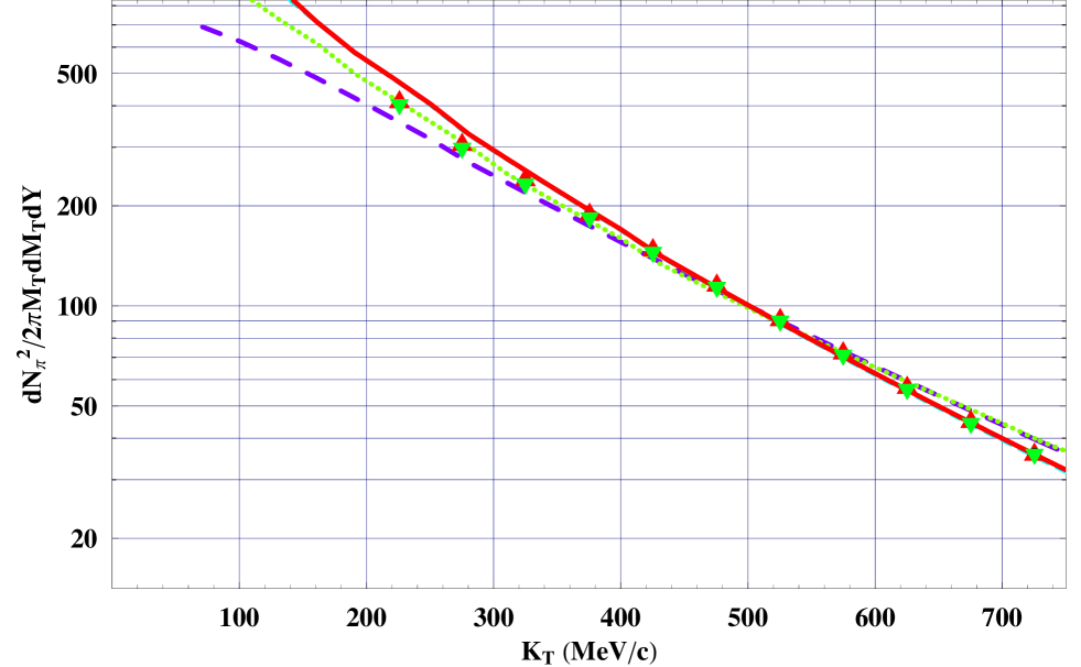
Figure 1: Color online. Computed pionic spectrum. Red upright triangles: $\pi^{-}$ spectrum (STAR) Green inverted triangles: $\pi^{+}$ spectrum points (STAR) Adams:2003xp Red solid line: DWEF fit with vanishing imaginary part of the optical potential, first line of Table I. Green dotted line: DWEF fit including search on the imaginary part of the optical potential, second line of Table I. Blue dashed line(almost entirely covered by the red solid curve): DWEF fit with vanishing imaginary part of the optical potential,$\Delta\tau$ = 1.5 fm/c, third line of Table I. Violet long dashed line: DWEF fit including search on $\mu_{\pi}$, setting the optical potential to essentially 0, fourth line of Table I.

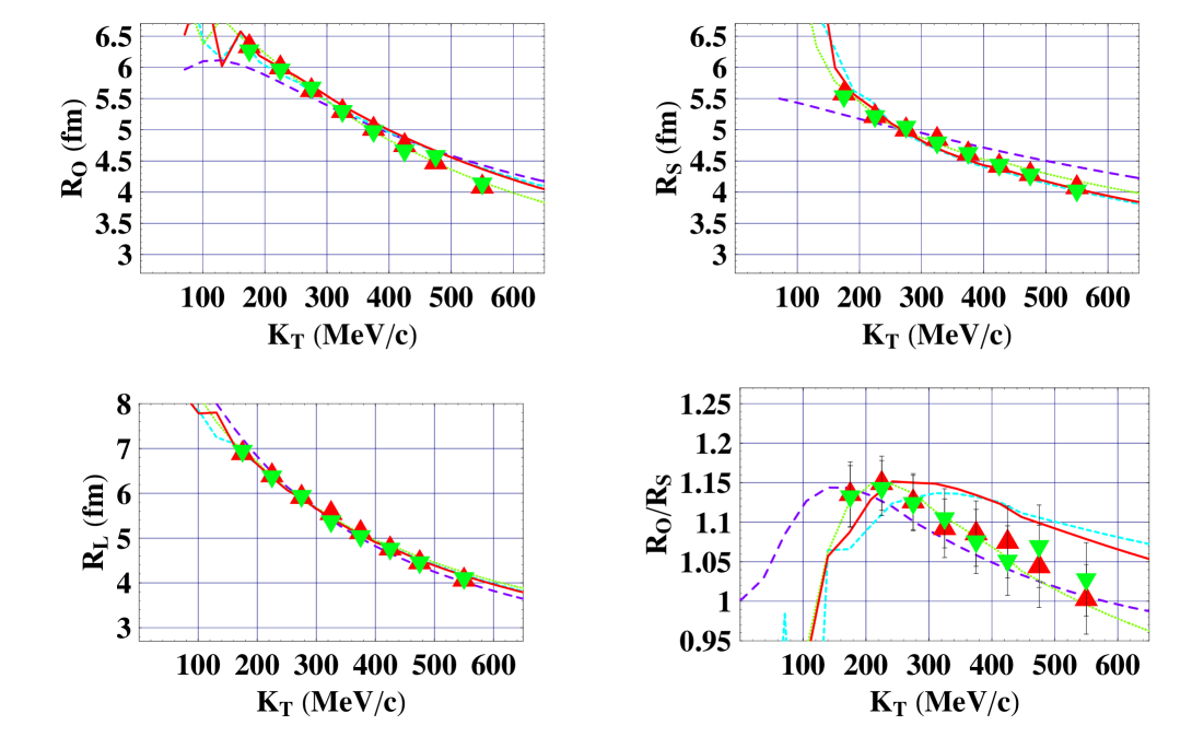
Figure 2: Color online. HBT radii. Curves are labeled as in Fig. 1. STAR data Adams:2004yc

Table 1: Four parameters sets obtained with slightly different procedures. These parameters are defined in Miller:2005ji . The values of $\chi^{2}$ represents the accuracy of the description of the data.

$T(MeV)$	$\eta_{f}$	$\Delta\tau(fm/c)$	$R_{WS}(fm)$	$a_{WS}(fm)$	$w_{0}(fm^{-2})$	$~{}w_{2}$	$\tau_{0}(fm/c)$	$\Delta\eta$	$\mu_{\pi}(MeV)$	$\chi^{2}$
121	1.05	0	11.7	1.11	0.495	0.762 +0.0001$i$	9.20	70.7	139.57	300
162	1.22	1.55	11.9	1.13	0.488	1.19+0.13$i$	9.10	1.68	139.57	117
121	1.04	1.5	11.7	0.905	0.564	0.595 +0.0001$i$	8.85	70.7	139.57	451
144	0.990	2.07	12.57	0.876	0.0001	0.0001+ 0.0001$i$	6.85	$\infty$	83.5	1068

VI Summary and Discussion

It seems clear from previous work including Gyulassy -th and the present Sect. III that final state interaction effects on HBT interferometry are appropriately included by solving quantum mechanical wave equations. However, if the optical potential has an imaginary part, there is an additional effect, embodied in Eq. (51) that needs to be included when computing the emission probabilities and correlation function. Thus the effects of strong quantum opacity must be accompanied by additional pion emission from the states eliminated in the construction of the complex optical potential. In the work of Cramer:2004ih ; Miller:2005ji the real part of the optical potential is very important and the imaginary part of the optical potential is a small effect. However, obtaining a similarly accurate reproduction of the pionic spectra and HBT radii without this imaginary part causes the emission temperature to drop from about 160 MeV to 120 MeV and the fitted emission duration time to drop to 0. This indicates that, in our model, either the final state interactions occur in the later times of the collision and that the emission occurs at only one proper time, or the inclusion of emission from the states eliminated in the construction of the complex optical potential is necessary.

- (1) S. Pratt, “Two Particle And Multiparticle Measurements For The Quark - Gluon Plasma,” in Hwa, R.C. (ed.): Quark-gluon plasma, vol.2, page 700-748, 1995.
- (2) U. A. Wiedemann and U. W. Heinz, Phys. Rept. 319, 145 (1999).
- (3) P. F. Kolb and U. Heinz, Quark Gluon Plasma 3, edited by R.C. Hwa and X.-N. Wang, World Scientific, Singapore, 2004)
- (4) M. Lisa, S. Pratt, R. Soltz and U. Wiedemann, Ann. Rev. Nucl. Part. Sci. 55, 357 (2005)
- (5) S. Pratt, Phys. Rev. Lett. 53, 1219 (1984). G. F. Bertsch et al., Phys. Rev. C37, 1896 (1988).
- (6) D. H. Rischke and M. Gyulassy, Nucl. Phys. A 608, 479 (1996)
- (7) C. Adler et al. [STAR Collaboration], Phys. Rev. Lett. 87, 082301 (2001); K. Adcox et al. [PHENIX Collaboration], Phys. Rev. Lett. 88, 192302 (2002); A. Enokizono [PHENIX Collaboration], Nucl. Phys. A 715, 595 (2003).
- (8) U. W. Heinz and P. F. Kolb, hep-ph/0204061.
- (9) M. Gyulassy and L. McLerran, Nucl. Phys. A 750, 30 (2005).
- (10) J. G. Cramer, G. A. Miller, J. M. S. Wu and J. H. S. Yoon, Phys. Rev. Lett. 94, 102302 (2005). Erratum ibid Phys. Rev. Lett. 95, 139901(E) (2005).
- (11) G. A. Miller and J. G. Cramer, J. Phys. G 34, 703 (2007) .
- (12) M. Gyulassy, S. K. Kauffmann and L. W. Wilson, Phys. Rev. C 20, 2267 (1979)
- (13) H. W. Barz, Phys. Rev. C 53, 2536 (1996).
- (14) H. Heiselberg and A. P. Vischer, Eur. Phys. J. C1, 593 (1998)
- (15) B. Tomasik and U. W. Heinz, Acta Physica Slovaca 49, 251 (1999)
- (16) H. W. Barz, Phys. Rev. C 59, 2214 (1999) [arXiv:nucl-th/9808027].
- (17) J. I. Kapusta and Y. Li, Phys. Rev. C 72, 064902 (2005) [arXiv:nucl-th/0503075].
- (18) C. Y. Wong, J. Phys. G 29, 2151 (2003)
- (19) S. Pratt, Phys. Rev. C 77, 014609 (2008)
- (20) R. Hanbury Brown and R.Q. Twiss, Nature 178,1046 (1956)
- (21) G.I. Kopylov, Phys. Lett. 50B, 472 (1974)
- (22) P. Danielewicz, Phys. Lett. B 274, 268 (1992)
- (23) J. Adams et al. [STAR Collaboration], Phys. Rev. C 71, 044906 (2005).
- (24) J. Adams et al. [STAR Collaboration], Phys. Rev. Lett. 92, 112301 (2004) [arXiv:nucl-ex/0310004].
- (25) F. Retiere and M. A. Lisa, Phys. Rev. C 70, 044907 (2004) [arXiv:nucl-th/0312024].