Necessary conditions for accurate computations of three-body partial decay widths

Abstract

The partial width for decay of a resonance into three fragments is largely determined at distances where the energy is smaller than the effective potential producing the corresponding wave function. At short distances the many-body properties are accounted for by preformation or spectroscopic factors. We use the adiabatic expansion method combined with the WKB approximation to obtain the indispensable cluster model wave functions at intermediate and larger distances. We test the concept by deriving conditions for the minimal basis expressed in terms of partial waves and radial nodes. We compare results for different effective interactions and methods. Agreement is found with experimental values for a sufficiently large basis. We illustrate the ideas with realistic examples from $\alpha$-emission of ¹²C and two-proton emission of ¹⁷Ne. Basis requirements for accurate momentum distributions are briefly discussed.

I Introduction

The spectrum of a given many-body quantum system provides a set of characteristic observables: the energies and the widths. All quantum states, except perhaps the ground state, decay if sufficient time is available. For bound states, where the total energy is less than all thresholds for division into subsystems, only electromagnetic and particle transforming decays are possible. The first of these decays maintains the identity of the constituent particles in contrast to the latter exemplified by beta-decay where neutrons are transformed into protons or vice versa. However, if the energy is sufficiently high, the system can also decay into subsystems while maintaining the identity of the constituent particles. In this work, we shall concentrate on decays where the energy allows such fragmentation of the initial system.

In general we then have a many-body continuum problem. For nuclei the simplest final state consists of two fragments, e.g. two fission fragments, or a daughter nucleus plus a nucleon or an $\alpha$-particle gam28 . If both initial and final states are completely specified, energy and momentum conservation determine the relative kinetic energy between the two outgoing particles. The decay rate (or the width found by multiplying the rate by $\hbar$) is obtained from preformation, or spectroscopic factors, combined with the probability for tunneling through the barrier in the relative potential created by the two-body interaction. This barrier separates the short-distance initial many-body state from the large-distance final two-body state kra88 . The many-body problem is reduced to a two-body problem where only the two particles found after the decay appear.

Larger widths may be found in more elaborate models exploiting different, perhaps virtual, configurations resulting in a coupled channels problem alk03 . Such relatively simple two-body decays have been studied from the beginning of the history of quantum mechanics, exemplified by $\alpha$-emission gam28 . Similar processes vary from statistical emission of nucleons above the nucleon separation energy for ordinary nuclei bon95 , to (almost) instant decay outside the neutron dripline and to proton and $\alpha$-emission outside the proton dripline tho04 ; bla08 .

In this work we shall consider decay processes where three fragments are found in the final state. This is the simplest, yet not understood, extension of the concept of two-body decay fed03 . Furthermore, to limit the number of possible final states we assume that the three-body threshold is lower than any other threshold. Energy and momentum conservation still provide constraints, but the internal distribution of the total momentum and energy between the three fragments is not decided by these conservation laws. These momentum and energy distributions are observables carrying detailed information about the initial state and the process. Reliable computations require accurate determination of the large-distance properties of the cluster wave functions alv07 ; rod07 . On the other hand, the decay width is an average quantity which is very sensitive to properties of the potential barrier, but in analogy to two-body decay, it is determined by the effective barrier at small and intermediate distances.

Nowadays, different methods to compute the partial decay width into three specified fragments are already available gar04 ; rod07 ; gri00 . However, the conditions for their reliability and suitability are not well established, and each method is most often rather tested on the individual systems under investigation. The discussions comparing the different methods are deceivingly mixing effects of choices of (i) degrees of freedom, (ii) interactions, (iii) theoretical method, and (iv) numerical convergence. Untangling these effects is badly needed to formulate necessary conditions for accurate computations. Benchmark computations for precisely specified systems and interactions would be valuable as test criteria for reliability of the methods.

The purpose of the present paper is to provide verifiable simple but revealing test examples. To do this it is necessary to separate and assess the impact of each of the effects (i)-(iv). We first explain why the basic ingredient for partial three-body decay widths necessarily must be a three-body cluster model. We shall formulate necessary conditions for accurate three-body computations, and document by numerical applications on realistic three-body decaying systems. It is crucial that extensions to include more complicated effects are built on methods which are established as accurate.

The basic concepts for three-body decay widths are in section 2 described and tested against measured results. In section 3 we give analytical estimates of the quantities characterizing the crucial potentials and the basis size needed for accurate computations. In section 4 we test the estimates with the clean example of the Hoyle resonance in ¹²C. We then discuss in section 5 how the computed widths depend on the basic interactions and the available methods. We also briefly discuss the more severe accuracy requirements for momentum distributions determined at larger distances. Finally section 6 contains summary and conclusions.

II Framework

Different definitions exist of the decay width, e.g. in terms of cross sections tay72 , or phase shifts and $S$-matrix poles fri91 , or eigenvalues of the Hamiltonian $H$ lan65 . We shall use the width of a given resonance defined as minus two times the imaginary part of the generalized eigenvalue of the Hamiltonian. This is equivalent to a pole in the $S$-matrix at the complex momentum corresponding precisely to that eigenvalue. This definition is only complete after specification of the degrees of freedom contained in $H$. The full many-body Hamiltonian would give the total width, while confined to three particles in the final state the result is an approximation to the corresponding partial decay width.

II.1 Basic concept

The important issue in three-body decays is that the many-body degrees of freedom must be (re)organized into intrinsic and relative cluster coordinates. This division is usually not meaningful at small distances when all particles are close and within the nuclear volume. In contrast, this is the only meaningful division at large distances where three free particles are present. The quantum mechanical wave function must reflect this transition and the three-body structure at large distance must unfold into a many-body structure at small distance. To get a correct partial three-body width, effects from the small distances must be incorporated, e.g. by a preformation factor and the assumption of an artificial attractive pocket designed to provide both the correct energy and the resonance small-distance boundary condition. This treatment is precisely as for $\alpha$-emission in the classical Gamow theory gam28 ; kra88 ; fed03 .

In practice the many-body problem is therefore transformed into a three-body problem for all distances. The potential pocket in three-body coordinates has to be added by hand, unless the chosen two-body interactions already are sufficient. It is crucial to have the correct three-body resonance energy as evident from the exponential energy dependence of the width determined from tunneling probability through any barrier. Thus we have to insist on a practical method to adjust the energy to the correct value, e.g. by use of a short-range three-body interaction fed96 . This separates the model dependence of short-distance many-body structure from effects of the three-body cluster model at intermediate distances. In Gamow theory this is achieved by adding an attractive $\alpha$-daughter interaction, e.g. a square-well or Woods-Saxon potential with a radius about the size of the nucleus.

All methods to compute partial three-body decay widths must at some point address this separation of distances, degrees of freedom and related effective interactions. However, the procedures to reach the reduction into the three-body structure are rather different. Microscopic derivations start from nucleon-nucleon interactions and integrate away the unwanted degrees of freedom while simultaneously leaving corresponding effective interactions kam07 ; des01 ; ara03 ; kan07 ; nef04 . The mean-field model is also used for two-proton decay in the formulation named the Gamow shell-model where the nucleon degrees of freedom are present and the interactions are phenomenological adjusted within the mean-field mic02 ; bet02 ; oko03 .

If the three-body cluster model is assumed from the beginning for all distances, the corresponding two-body interactions are usually obtained from phenomenological adjustments to two-body data. No matter how the effective two-body interactions are found, they are much more important in three-body than in two-body decays. For example for $\alpha$-emission, the distance between $\alpha$-particle and daughter quickly leaves only non-vanishing contributions from Coulomb and centrifugal forces alv07 ; rod07 . For three-body decay, where two particles stay close while the third particle moves away, the short-range interactions contribute much more to the properties of the decisive barrier gar04 .

The crux of the matter is then to deduce the partial decay width from the three-body cluster model for a given resonance energy. Here several methods have been employed. The practical and experiment oriented method is to use elastic scattering cross sections as function of energy tay72 ; fri91 . A peak is then related to a resonance and its width is the resonance width. However, this is not practical for collisions of more than two particles, and furthermore uncertainties arise from corrections due to phase space distortion, broad peaks, overlapping resonances, background contributions, etc. We prefer the more mathematical definitions of a complex pole in the $S$-matrix fri91 , or the energy derivative of the scattering phase shift while crossing through $\pi/2$ tay72 ; fri91 , or equivalently minus twice the imaginary part of the eigenvalue of the hamiltonian lan65 , or equivalently related to the solution of complex energy with an outgoing flux in all channels.

The numerical method to compute the complex resonance energy has to allow for complex energy solutions and for example insist on only an outgoing flux in all channels ara96 . Equivalently all coordinates can be rotated a given angle into the complex plane which turn the outgoing flux solution into an exponentially falling solution at large distances precisely as for bound states ho83 ; cso97 . Another method exploits analytic continuity of the interactions by varying with respect to for example the strength parameter tan99 ; tan99b . These methods are essentially all equivalent and produce identical results for identical interactions and the same Hilbert space.

A semiclassical perturbative method has been abundantly employed recently gri00 ; gri03 ; gri07 . It assumes that the width is small and related to the outgoing flux for the solution to the Schrödinger equation obtained by confinement to a box of finite extension. This method is presumably also equivalent to the other methods for narrow resonances when the perturbation assumption is valid.

II.2 Testing the concept

The bare problem can be envisaged as a potential and a corresponding wave function with resonance character conveniently described by a complex energy and only an outgoing flux. Real ($E_{R}$) and imaginary ($E_{I}$) parts of the energy are closely linked through the potential, e.g. adding a small positive potential at small distance would increase $E_{R}$, leave the potential barrier unchanged, and increase $|E_{I}|$ exponentially. We shall test the idea with the simplest computation of the width, $\Gamma=-2E_{I}$, i.e. by use of the WKB-approximation.

However, to do this, a potential defined as function of a generalized radial coordinate is required. The coordinates for three particles then should be combined into one overall important coordinate $\rho$ which on its own should be able to describe the process. We want to maintain the intuitive understanding that small $\rho$ means small physical distances between all three particle at the same time. Vice versa, large $\rho$ should be able to describe the structure after fragmentation into three particles. To give a precise and physically meaningful definition of $\rho$ in terms of the particle coordinates we assume a quadratic dependence on interparticle distances. Then the hyperradius $\rho$ is unique apart from the choice of mass weighting, where we use $mM\rho^{2}=\sum_{i<j}m_{i}m_{j}(\vec{r}_{i}-\vec{r}_{j})^{2}$, with $m_{i}$ and $\vec{r}_{i}$ as mass and coordinate of particle $i$, and $M=m_{1}+m_{2}+m_{3}$ mac68 ; nie01 . In our calculations we take the normalization mass $m$ equal to the nucleon mass.

We shall use $\rho$ as the generalized coordinate. In the spirit of the generator coordinate method, where the energy is calculated as function of one parameter, we solve the Schrödinger or Faddeev equations for each value of $\rho$ between zero and $\rho_{max}$. The hyperangular degree of freedom is automatically quantized as the solution to the corresponding Schrödinger equation, which for each $\rho$ takes the form:

$$\hat{\Lambda}^{2}\Phi_{n}(\rho,\Omega)+\frac{2m\rho^{2}}{\hbar^{2}}V(x)\Phi_{n}(\rho,\Omega)=\lambda_{n}(\rho)\Phi_{n}(\rho,\Omega),$$ (1)

where $\hat{\Lambda}$ is the hyperangular operator nie01 , $V$ is the sum of the three two-body potentials, and $\Omega$ represents the five hyperangles.

If we now use the complete set of solutions for each $\rho$ as basis ($\Psi={1\over\rho^{5/2}}\sum_{n}f_{n}(\rho)\Phi_{n}(\rho,\Omega)$) we arrive at the hyperspherical adiabatic expansion method, which reduces the problem to the following set of coupled differential equations in $\rho$:

$$\left[-\frac{d^{2}}{d\rho^{2}}+\frac{2m}{\hbar^{2}}(V_{3b}(\rho)-E)+\frac{1}{\rho^{2}}\left(\lambda_{n}(\rho)+\frac{15}{4}\right)\right]f_{n}(\rho)$$

$$+\sum_{n^{\prime}}\left(-2P_{nn^{\prime}}\frac{d}{d\rho}-Q_{nn^{\prime}}\right)f_{n^{\prime}}(\rho)=0,\;\;\;$$ (2)

where $E$ is the three-body energy, $V_{3b}$ is a three-body potential used for fine-tuning, and the functions $P_{nn^{\prime}}$ and $Q_{nn^{\prime}}$ are given for instance in nie01 .

These equations contain the effective adiabatic potentials, which take the form:

$$V_{\mbox{eff}}(\rho)=\frac{\hbar^{2}}{2m}\frac{\lambda_{n}(\rho)+15/4}{\rho^{2}}+V_{3b}(\rho).$$ (3)

The number of differential equations (or of adiabatic potentials) is equal to the size of the basis for each $\rho$. This basis is unique in the description of multifragmentation, because it is the only representation that maps fragmentation theory onto a set of coupled channel differential equations from two-body reaction theory mac02 ; mac68 .

To fix the concept we shall first only use the lowest of these adiabatic potentials which depend on angular momentum and parity of the three-body system. The three-body configurations change in a non-trivial manner from small to large hyperradii. The total energy, apart from the kinetic energy related to variation of $\rho$, is minimized for each $\rho$. However, $\rho$ does not uniquely determine even the geometric configuration. The same $\rho$ is related to continuously differing combinations of distances between the particles, e.g. a small distance between two particles and a large distance to the third particle, or equal distance between all particles, etc. Thus, it is not a priori obvious why this should be a good choice of coordinates for an efficient description of these decays. Other configurations might be important but this would be reflected in a finite population of the complete set of higher-lying adiabatic potentials.

Figure 1: The computed lowest adiabatic potential as function of hyperradius for a number of resonances of ¹²C ($\alpha$+$\alpha$+$\alpha$). The horizontal lines mark the resonance energies measured above the three-body threshold. The corresponding excitation energies are given above each of the panels ajz90 .

In Fig.1 we show the lowest adiabatic potentials for various angular momenta and parities $J^{\pi}$ in ¹²C ($\alpha$+$\alpha$+$\alpha$). The behavior of the three body systems is unpredictable from $J^{\pi}$ alone. A minimum at small distances indicates a substantial amount of cluster structure and vice versa, no minimum indicates dominance of many-body non-cluster structure often referred to as shell model structure. In all cases, after decay, the three alpha particles must emerge outside the barrier. The physical meaning of this description is different from the intuitive perception of a mean-field shell model where a monotonous dependence on excitation energy and angular momentum would be expected. Here the three-body structure and the properties of the two-body interactions are crucial and capable of changing the expected ordering.

The partial decay width must sensitively depend on the energy and the properties of the barrier which must be crossed. The complex energy solutions of the hyperradial equation give the widths, which we here estimate by the WKB tunneling probabilities through the one-dimensional potential barriers. We fix the real part of the energies equal to the measured values whenever they are available. This can be achieved by using an appropriate three-body short-range attractive potential ($V_{3b}(\rho)$ in Eq.(2)). A simple form of this is employed in Fig.1, where we take a square well potential of radius $4$ fm and a depth adjusted to give the experimental resonance energies.

Figure 2: The computed widths compared to the measured values for different resonances of ¹²C with excitation energy $E^{*}$ ajz90 . The WKB approximation is used for tunneling through the lowest adiabatic potential where the inner turning point is fixed to a hyperradius of $\rho=4$ fm.

The WKB estimates are obtained from the action integral between the classical turning points determined by the real part of the energy ($E$). The transmission coefficient is then given by:

$$T=\exp{\left\{-2\int_{\rho_{i}}^{\rho_{t}}\left[\frac{2m}{\hbar^{2}}(V_{\mbox{eff}}(\rho)-E)\right]^{1/2}d\rho\right\}}\;,$$ (4)

where $\rho_{i}$ and $\rho_{t}$ are the inner and outer classical turning points defining the distance through the barrier. Once the transmission coefficient is computed, the decay constant can be obtained as $\Gamma/\hbar$=$fT$, where $f$ is the knocking rate.

The results are shown in Fig.2 where only a factor of 2-5 remains to match the measured values which vary by about 5 orders of magnitude with only a variation of 7 MeV in excitation energy $E^{*}$. The smallest widths occur for the smallest angular momenta but the largest widths do not occur for the largest angular momenta. The only exception is the lowest $1^{+}$ state where the computed width is too small by about a factor of $100$. The reason is that the large-distance tail of the corresponding potential sensitively contributes to the width for this state, see Fig.1. The basis size should then in this case have been larger than used to obtain this estimate.

In more accurate computations, as discussed in details in this report, the inner turning point would also be larger implying larger computed widths. This would in turn indicate reduction due to preformation, or spectroscopic, factors, arising from a short-distance structure deviating from that of three $\alpha$-particles. In any case, we can conclude that the use of the hyperradius as the generating coordinate is valid to account for the main dependencies of the resonance widths on the excitation energy and angular momentum and parity of the system.

III Crucial ingredients

The exponential dependence of the widths on the properties of the confining barrier immediately emphasizes that the most crucial ingredient is the potential barrier which must be accurately determined between classical turning points. Any inaccuracies would be exponentially enhanced in the width computation. Thus, it is essential first to know the coordinate region where accuracy is indispensable which means that the turning points should be found. Second, it is crucial to control the numerical technique responsible for the computation of the potential barriers in this coordinate range.

III.1 Turning point estimates

The inner turning point is at a distance where the short-range interaction is most important. It is sensitive to the details of the potential and the energy and quantum numbers of the resonance. However, the short distance allows accurate computation without too many difficulties, provided that the cluster division is assumed and the many-body problem reduced to that of three particles.

Then the outer classical turning point is an estimate of the largest distance needed in accurate computations. If we assume that only repulsive Coulomb interactions remain at these distances we can use hyperradial coordinates and find the turning point $\rho_{t}$ with the formalism developed in gar05 .

When a direct decay of the three-body system is assumed, all relative two-body distances scale proportionally. We can then minimize the action integral and arrive at the general expression gar05

$$\rho_{t}=\frac{e^{2}}{E\sqrt{mM}}\left(\sum_{i<k}(z_{i}z_{k})^{2/3}(m_{i}m_{k})^{1/3}\right)^{3/2}$$ (5)

where $ez_{i}$ is the charge of particle $i$ and $E$ is the energy of the three-body resonance which at the turning point equals the potential energy.

The partial waves necessary to describe this distance can be estimated from the fact that at the turning point the value of the potentials can not be higher than the three-body energy $E$. Therefore, the centrifugal barrier must be smaller than $E$ at the turning point, i.e.

$$\frac{\hbar^{2}}{2m}(\frac{\ell_{x}(\ell_{x}+1)}{x^{2}}+\frac{\ell_{y}(\ell_{y}+1)}{y^{2}})<E\;,$$ (6)

where $x$ and $y$ are the usual Jacobi coordinates, and $\ell_{x}$ and $\ell_{y}$ are relative angular momenta related respectively to the distance between two particles and their center of mass and the third particle. Assuming that both the total angular momentum and the intrinsic spins are small, we have $\ell_{x}\approx\ell_{y}$, and for sufficiently large values of $\ell_{x}$ and $\ell_{y}$ we can take $\ell_{x}(\ell_{x}+1)\approx\ell_{x}^{2}$ and $\ell_{y}(\ell_{y}+1)\approx\ell_{y}^{2}$. Furthermore $x$ is proportional to the distance between two of the particles, say $1$ and $2$, and for a direct decay all distances between pairs of particles are similar. This leads to

$$x\approx\rho_{t}\sqrt{\frac{M\mu_{12}}{\sum_{i<k}m_{i}m_{k}}}\;\;\;,\;\;\;y\approx\sqrt{\rho_{t}^{2}-x^{2}}$$ (7)

with $\mu_{12}=\frac{m_{1}m_{2}}{m_{1}+m_{2}}$, from which one gets

$$\ell_{x}\approx\ell_{y}<\frac{\rho_{t}}{\hbar\sum_{i<k}m_{i}m_{k}}\sqrt{2EmMm_{1}m_{2}m_{3}}\>.$$ (8)

Two limits of Eqs.(5) and (8) are useful in practice. When all particles have the same masses $m_{0}$ and charges $z_{0}$ we find

$$\rho_{t}\approx\frac{3z_{0}^{2}e^{2}}{E}\sqrt{\frac{m_{0}}{m}}\;\;,\;\;\ell_{x}\approx\ell_{y}<z_{0}^{2}e^{2}\sqrt{\frac{6m_{0}}{\hbar^{2}E}}\;.$$ (9)

When particle $3$ has mass $m_{3}$ and charge $z_{3}$ much larger than for the other two particles, i.e. $m_{1}\approx m_{2}\ll m_{3}$ and $z_{1}\approx z_{2}\ll z_{3}$, we obtain

$$\rho_{t}\approx\frac{z_{1}z_{3}e^{2}}{E}\sqrt{\frac{8m_{1}}{m}}\;\;,\;\;\ell_{x}\approx\ell_{y}<2z_{1}z_{3}e^{2}\sqrt{\frac{m_{1}}{\hbar^{2}E}}\;.$$ (10)

Notice here that the estimates of lengths in hyperspherical coordinates always are combined with the normalization mass $m$, e.g. only $\rho_{t}\sqrt{m}$ is expressed in terms of physical parameters like particle energies, masses and charges. In contrast dimensionless quantities like the angular momenta in Eqs.(9) and (10) do not involve the arbitrary mass $m$.

Instead of following a path where all distances scale proportionally it could be advantageous to tunnel through the barrier by exploiting the two-body attraction between two particles while the third particle moves away. This is a sequential decay where the geometry reduces the Coulomb interactions and supplies additional energy from the short-range interaction. In total the barrier could be substantially smaller both in height and width. If the intermediate two-body configuration carries an energy $E_{12}$ we find

$$\rho_{t}\approx\frac{z_{3}(z_{1}+z_{2})e^{2}}{(E-E_{12})}\sqrt{\frac{m_{3}(m_{1}+m_{2})}{mM}}\;$$ (11)

$$\ell_{y}<z_{3}(z_{1}+z_{2})e^{2}\sqrt{\frac{2m_{3}(m_{1}+m_{2})}{M\hbar^{2}(E-E_{12})}}\;.$$ (12)

Where we have used that for sequential decay large values of $\rho$ imply $\rho\approx y$, and the relative distances $r_{31}$ and $r_{32}$ are similar to $r_{12,3}=y\sqrt{m/\mu_{12,3}}\approx\rho\sqrt{m/\mu_{12,3}}$. The angular momentum estimate is an upper limit because the two-body attraction can typically only be exploited for one or very few given small values of $\ell_{x}$ which by angular momentum conservation also forces $\ell_{y}$ to have a small value.

In the two limits of the same masses ($m_{0}$) and charges ($z_{0}$), and one mass and charge ($m_{3}$ and $z_{3}$) much larger than the other two ($m_{1}\approx m_{2}$ and $z_{1}\approx z_{2}$), we find that

$$\rho_{t}\approx\frac{2z_{0}^{2}e^{2}}{(E-E_{12})}\sqrt{\frac{2m_{0}}{3m}}\;\;,\;\;\ell_{y}<\sqrt{\frac{16m_{0}(z_{0}^{2}e^{2})^{2}}{3\hbar^{2}(E-E_{12})}}\;,$$ (13)

$$\rho_{t}\approx\frac{2z_{3}z_{1}e^{2}}{(E-E_{12})}\sqrt{\frac{2m_{1}}{m}}\;\;,\;\;\ell_{y}<\sqrt{\frac{16m_{1}(z_{3}z_{1}e^{2})^{2}}{\hbar^{2}(E-E_{12})}}\;.$$ (14)

The balance between the smaller Coulomb energy and the additional two-body energy $E_{12}$ determines whether the tunneling process is direct (all pairs of particles are outside their short-range attraction at the turning point and all distances scale proportionally) or sequential (the attraction from one or more pairs of particles is used as vehicle to speed up the process by tunneling through a smaller barrier). Different paths can contribute to the same decay process. The dominating path would typically correspond to the smallest outer turning point $\rho_{t}$.

III.2 Basis requirements

The width can only be accurately computed if the potential and the related wave functions are accurate up to at least the true outer turning point. For this it is important that the Hilbert space is sufficient to allow the system to choose the optimum path through an accurately determined barrier. This in turn can only be achieved when the numerical procedure allows a precise coherent description of all two and three-body intermediate configurations.

For coherently contributing two-body substructures this is only ensured by Faddeev, or Faddeev-like, decompositions. One set of Jacobi coordinates is obviously simpler than including all three Faddeev components but it also has a tremendous disadvantage for systems where more than one two-body subsystem simultaneously have bound or nearly bound states, and especially when relatively large distances are important. The Efimov effect is for example completely excluded from the description in a basis of one Jacobi set of coordinates.

In many computations basis expansions are exploited. With the hyperradius as coordinate the natural basis is hyperharmonics for each Jacobi set in the basis. To describe structures varying over distances comparable to the range of the two-body interaction, $b_{12}$, the basis must on average contain a few points within that distance. For a given $\rho$ the two-body distance is $r_{12}=\sqrt{m/\mu_{12}}x$ ($x\equiv\rho\sin\alpha$), which means that a proper description of the internal two-body structures for large $\rho$’s requires basis terms with nodes within the small region $0\leq\alpha\leq\sqrt{\mu_{12}/m}\;b_{12}/\rho$. The number of nodes between 0 an $\pi/2$ of a given hyperspherical harmonic is given by the principal quantum number $n$ of the Jacobi polynomial contained in it. This means that a typical separation between nodes is $\pi/(2n)$. Therefore, to have at least one node below $\sqrt{\mu_{12}/m}\;b_{12}/\rho$ one needs

$$n>\frac{\pi}{2}\frac{\rho}{b_{12}}\sqrt{\frac{m}{\mu_{12}}},$$ (15)

which implies that the maximum hypermomentum quantum number $K_{max}$ ($=2n+\ell_{x}+\ell_{y}$) should at least exceed a lower limit, i.e.

$$K_{max}>\frac{\pi\rho}{b_{12}}\sqrt{\frac{m}{\mu_{12}}}+\ell_{x}+\ell_{y}\;,$$ (16)

where we assumed given hyperradius and partial angular momenta. Thus the number of basis functions, or $K_{max}$, must increase proportional to $\rho$. The proportionality factor providing the unit of $\rho$ for this estimate is inversely proportional to the range of the two-body interaction which initially is responsible for the structures we try to describe. The minimum basis size can only be found in practice by numerical calculations.

When the turning point, $\rho=\rho_{t}$, is needed we can insert the expression in Eq.(5) in Eq.(16). Then only the physical parameters remain in the estimate of $K_{max}$. Furthermore, to relate $\rho_{t}$ to the physical size of the system the definition of the hyperradius can be used, which leads to $m\rho_{t}^{2}\approx r_{av}^{2}\sum_{i<k}m_{i}m_{k}/M$ where $r_{av}^{2}$ is an appropriate average of the distance, $(\vec{r}_{i}-\vec{r}_{j})^{2}$, between pairs of particles.

IV A test case: The Hoyle state in ¹²C.

We consider here the Hoyle state, i.e. the first $0^{+}$ resonance in ¹²C described in terms of three $\alpha$-particles, which is the only possible particle decay mode. The intrinsic $\alpha$-particle spins are zero and the wave function must be symmetric with respect to all interchanges of pairs of particles. This limits the number of necessary partial waves and the $K_{max}$-dependence of the effective potential and wave function can conveniently be investigated.

The well-studied converged result is known to be a narrow resonance with a width of only 8.5 eV at an energy of 0.38 MeV. A detailed calculation using the hyperspherical adiabatic expansion method can be found in rod07 where the structure is shown to arise essentially from only one of the adiabatic potentials.

Following the estimates in Eq.(9) where a direct decay is assumed, we obtain an estimated value for the outer turning point of $\rho_{t}\approx 90$ fm, while the maximum values for the two-body relative orbital angular momenta are $\ell_{x}\approx\ell_{y}\approx 7$. However, the proportional scaling of all distances is inefficient because the two-body attraction is not exploited while the full Coulomb repulsion is encountered. By using Eq.(13) instead we find $\rho_{t}\approx 67$ fm with $E_{12}=0.1$ MeV as the energy of the ⁸Be subsystem, and $\ell_{y}\approx 8$. The coherence of all three subsystems reduces the turning point and keeps the number of components. Then the barrier is reduced and this escape mechanism is preferred. For the second case ($\rho_{t}\approx 67$ fm and $\ell_{y}\approx 8$), and following (16), we get that $K_{max}$ has to be about 80 in order to ensure a proper treatment of the ⁸Be structure up to the outer turning point.

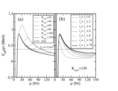
Figure 3: The dominating effective adiabatic potential for the lowest 0⁺ resonance in ¹²C ($\alpha$+$\alpha$+$\alpha$) for (a) different values of $K_{max}$ and (b) different values of partial waves in the expansion in terms of HH. The dashed straight line indicates the energy of the resonance. In (a) all the the possible values of $\ell_{x}$ and $\ell_{y}$ consistent with $K_{max}$ have been included. The curve called “full” includes $\ell_{x}=\ell_{y}$ up to 12 only and $K_{max}$=150, but with $K_{max}$ increased up to 500 for some of the components. In (b) $K_{max}$ is taken equal to 150.

In the left part of Fig.3, we show the lowest adiabatic effective potential for the $0^{+}$ states in ¹²C for different values of $K_{max}$. The dashed straight line indicates the energy of the resonance. In this calculation all the possible values of $\ell_{x}$ and of $\ell_{y}$ consistent with a given $K_{max}$ have been included. The curve quoted as full has been computed with $K_{max}$=150 and values of $\ell_{x}$ and $\ell_{y}$ up to 12 only, but increasing $K_{max}$ up to 500 for the most contributing components. As seen in the figure, the computed potential barrier (and the outer turning point) changes dramatically with $K_{max}$, and, in agreement with the estimate of Eq.(16), a $K_{max}$ value of at least 80 is needed in order to obtained a converged potential up to the outer turning point, which is found to be 60 fm (also in agreement with the estimated value).

In the right part of the figure we show the same effective potential for a fixed value of $K_{max}$ (we have taken 150), but where the values of $\ell_{x}$ and $\ell_{y}$ are progressively increased. It is clear from the figure that too small values of $\ell_{x}$ and $\ell_{y}$ produce a too small potential barrier. As estimated above, values of $\ell_{x}$ and $\ell_{y}$ of at least 8 are needed to match the thick curve, which is the one plotted in the right part with $K_{max}=150$ and with values of $\ell_{x}$ and $\ell_{y}$ of up to 74.

It is then clear from Fig.3 that simultaneous use of appropriate $K_{max}$ and maximum values of $\ell_{x}$ and $\ell_{y}$ are sufficient to reproduce accurately the potential barrier up to the outer turning point. This is the decisive region of the potential determining the width of a given resonance. It is important to note that while a too small value of $K_{max}$ overestimates the potential barrier, too small values of $\ell_{x}$ and $\ell_{y}$ underestimate it. Therefore both effects tend to compensate each other, in such a way that a poor calculation using too low $K_{max}$ and too few $\ell_{x}$ and $\ell_{y}$ could however luckily give a computed width not too far from the correct one.

Table 1: WKB estimates for the width of the lowest 0⁺ resonance in ¹²C for the seven effective potentials shown in Fig.3a (left part of the table) and for the seven potentials shown in Fig.3b (right part of the table). The column labeled as $\Gamma_{pert}$ refers to the widths obtained with the perturbative method described in gri00 . All the widths are given in MeV. The experimental value is $8.5\cdot 10^{-6}$ MeV.

$K_{max}$		$\Gamma_{WKB}$	$\Gamma_{pert}$	$\ell_{x}$,$\ell_{y}$		$\Gamma_{WKB}$
20		$3.6\cdot 10^{-11}$	$1.7\cdot 10^{-12}$	$=0$		$3.1\cdot 10^{-3}$
40		$3.9\cdot 10^{-10}$	$1.4\cdot 10^{-11}$	$\leq 2$		$6.8\cdot 10^{-5}$
60		$2.7\cdot 10^{-9}$	$9.1\cdot 10^{-9}$	$\leq 4$		$1.5\cdot 10^{-5}$
80		$2.7\cdot 10^{-8}$	$3.9\cdot 10^{-8}$	$\leq 6$		$7.9\cdot 10^{-6}$
100		$3.0\cdot 10^{-6}$	$2.7\cdot 10^{-7}$	$\leq 8$		$6.3\cdot 10^{-6}$
150		$4.2\cdot 10^{-6}$	$7.4\cdot 10^{-6}$	$\leq 10$		$5.4\cdot 10^{-6}$
Full		$5.5\cdot 10^{-6}$	$5.2\cdot 10^{-6}$

The dependence of the width on the basis size is illuminating. In table 1 we give the computed WKB widths for the different effective potentials shown in Fig.3a (left part of the table) and Fig.3b (right part of the table). The conclusion is striking, an insufficient basis (small $K_{max}$ or small maximum values of $\ell_{x}$ and $\ell_{y}$) easily leads to widths overestimated or underestimated by $3-5$ orders of magnitudes. However the converged result agrees reasonably well with the experimental value of $8.5$ eV. One has to keep in mind that only the uncertainty arising from the different possible choices of the knocking rate when computing the WKB width can easily produce variations in the width of up to a factor of 2 or 3. In our calculations we have taken the knocking rate equal to the energy of the resonance divided by the Plank constant ($E=h\nu$). Furthermore, in this estimate we have neglected the higher lying adiabatic potentials which typically contribute about 10-15% of the wave function. In any case, the width is exponentially depending on the barrier, and we have therefore demonstrated how catastrophic it is to use an insufficient basis.

A sufficiently large basis for three-body quantities is already important for structure computations of weakly bound halo systems jen04 . Excitations into the continuum of two-neutron halos, where the Coulomb interaction is absent, give more sensitivity and the opportunity to compare computations with measured strength functions. The inadequacy of a small basis was exhibited in fed97 for the $1^{-}$ excitation of the ⁶He ground state. This was further emphasized in the fairly successful prediction of the similar $1^{-}$ strength function for ¹¹Li in gar02 which later on was accurately measured in nak06 .

V Interactions and methods

For $\alpha$-emission it is well-known that the long-range interactions (as the Coulomb potential) and the centrifugal forces, by far have the largest influence on the decay rates. This is less obvious for three-body decays since the potential barriers depend on the two-body interactions. On the other hand the decay rate should be independent of the method adopted for the computations. This does of course assume that the methods are mathematically and/or physically equivalent which not always is easy to confirm.

V.1 Interaction dependence

An asymmetric and numerically more difficult system is found in ¹⁷Ne (¹⁵O+$p$+$p$), which provides an example of an exceedingly long-lived two-proton decaying state. This nucleus has a resonance with spin and parity 3/2^- with an energy of 0.34 MeV above threshold. The ground state of ¹⁶F (¹⁵O+$p$) is a resonance at 0.53 MeV above threshold. Decay of the 3/2^- resonance in ¹⁷Ne via a ¹⁶F resonance is then not allowed due to energy conservation. Also, core mass and charge are substantially larger than the values of the valence particles, meaning that the estimates of Eqs.(10) are applicable. From them we get $\rho_{t}\approx 96$ fm and $\ell_{x}<6$. From Eq.(16) we then estimate that $K_{max}\approx\rho_{t}/$(1 fm), i.e. to reach an accurate turning point when the two-body channels are exploited we can expect $K_{max}$-values of about 100.

The numerical difficulties are related both to less symmetry due to the presence of non-identical particles and the non-zero intrinsic spins of $1/2$ of all three particles. The number of partial waves are then immediately rather large due to the many allowed spin couplings. The most important interactions for the resonance structure are the $s$, $p$ and $d$-waves of the proton-¹⁵O system, each producing two low-lying resonances in ¹⁶F.

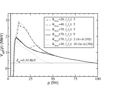
Figure 4: Lowest adiabatic effective potential for the 3/2^- resonance in ¹⁷Ne. Except for the last curve (thick-dot), the $p$-¹⁵O interaction is the one described in gar04 . The different curves correspond to calculations with different values of $K_{max}$ and relative two-body angular momenta. The thin-dotted curve corresponds to the calculation presented in gar04 . In the last (thick-dotted) curve, the $p$-¹⁵O potential and $K_{max}$ value of ref.gri03 have been used. The dashed straight line indicates the resonance energy of 0.34 MeV.

The lowest adiabatic effective potential for the 3/2^- resonance is shown in Fig.4. Except for the last case in the figure legend (thick-dotted curve) all the calculations have been performed using the interactions in gar04 . We notice the same pattern as in Fig.3, i.e. increasing $K_{max}$ up to values of about $70$ is required for convergence of the effective potential up to the outer turning point. This turning point appears at about 90 fm, in agreement with the estimation from Eq.(10). Otherwise the barrier is overestimated, giving rise to too small resonance widths. Also, the number of partial waves needed to obtain a proper convergence is relatively small ($\ell_{x}$ and $\ell_{y}$ values not bigger than 5 is enough, also in agreement with the estimation from Eq.(10)). If only $s$, $p$, and $d$-waves are used, the barrier (as illustrated by the thin-dotted curve) is too small, and consequently the computed width is too big. This barrier is the one used in ref.gar04 where a resonance width of $3.6\cdot 10^{-12}$ MeV was obtained. The true width is therefore expected to be a few orders of magnitude smaller than this number.

The thick dotted curve in Fig.4 has been obtained with $K_{max}=20$ and including all the partial waves consistent with this value, in total corresponding to the same Hilbert space as in gri03 . This curve is also obtained with the same interactions as in gri03 where a width of $4.1\cdot 10^{-16}$ MeV is quoted. This width is consistent with the $5.4\cdot 10^{-16}$ MeV obtained with the WKB approximation for this potential. However, as seen in the figure the barrier is substantially overestimated compared to the results with a much larger basis. The implication is that the width should be bigger than this number.

In Fig.4, the thick solid line corresponds to a calculation with $\ell_{x},\ell_{y}\leq$ 9, and $K_{max}$=70 for all the partial waves, except for those of large amplitude where $K_{max}$ values between 130 and 160 are used. Then the potential barrier shows the correct convergence properties and the WKB width for this potential and the resonance energy of $0.34$ MeV is found to be $1.7\cdot 10^{-14}$ MeV. This value is, as expected, in between the two given in gar04 and gri03 , and consistent with the corrected width of $(5-8)\cdot 10^{-15}$ MeV obtained in gri07 for a larger $K_{max}$ value. As seen in the figure, an increase of $K_{max}$ up to 40 improves significantly the calculated effective potential, although the barrier is still a bit overestimated. It it important to keep in mind the limitations inherent to the WKB approximation. Only one adiabatic potential is included, and additional inaccuracy arises from the definition used for the knocking rate and the fact that a preformation factor of unity is used.

The potentials shown in Fig.4 are to a large extent determined by the Coulomb and centrifugal potentials. This is understandable, since many of the crucial properties are determined at distances larger than the ranges of the short-range interactions. To investigate the dependence on these two-body interactions we can compare the results arising from the two potentials obtained with $K_{max}$=20. The first of them (long-dashed-dot curve) has been obtained with the proton-¹⁵O interaction given in gar04 , while the second one (thick-dot curve) uses the one in gri03 . These two interactions are very different, especially in their parametrization of the spin-dependence. In gar04 the spin-spin and spin-orbit operators are $\bm{s}_{c}\cdot\bm{j}_{p}$ and $\bm{\ell}\cdot\bm{s}_{p}$, where $\bm{j}_{p}=\bm{\ell}+\bm{s}_{p}$, $\bm{s}_{c}$ and $\bm{s}_{p}$ are the spins of the core and the proton, and $\bm{\ell}$ is their relative orbital angular momentum. In gri03 the more symmetric form of $\bm{s}_{c}\cdot\bm{s}_{p}$ and $\bm{\ell}\cdot(\bm{s}_{c}+\bm{s}_{p})$ is used.

The second set of spin-dependent operators in gri03 does not preserve the usual mean field quantum numbers corresponding to the core, and is as such inconsistent with the description of the protons in ¹⁵O. This symmetry breaking is especially problematic in cases where one spin-orbit partner is occupied by core nucleons while the other is available for the valence nucleons. Then the $d_{5/2}$ and $d_{3/2}$ resonances in ¹⁷Ne are mixed in the two-body description of the $1^{-}$ and $2^{-}$ resonances of ¹⁶F. In the three-body problem of ¹⁷Ne the two valence protons are then forced to partly occupy the same orbits. The Pauli principle between core and valence protons is violated and unwanted properties may appear, see gar03 for details. To compensate for these effects a fully phenomenological $J^{\pi}$ dependent three-body potentials are used but their effects on the widths could be rather unpredictable. An example of unwanted properties is seen in gri03 , where the potentials obtained with symmetry breaking spin operators are adjusted with three-body potentials to reproduce the known two-body spectrum in ¹⁶F. However, this simultaneously results in an additional $2^{-}$ resonance in ¹⁶F at 2.8 MeV with a width of 0.26 MeV. This resonance and the corresponding bound state in ¹⁶N at $-0.38$ MeV are not mentioned in the description of the interaction gri03 , and furthermore they are not known experimentally.

In Fig.4 it is shown how such exceedingly different two-body interactions lead to effective potentials in almost perfect agreement, provided that the same basis is used. Only a small difference is found around the inner turning point which is more sensitive to properties of the short-range interactions. This strongly indicates that the specific values of the energies of the two-body resonances are the only decisive quantities for the intermediate distances corresponding to the lowest adiabatic effective potential. Small-distance properties essential for spectroscopic factors as well as dynamic evolution of the resonance structures with distance due to couplings between potentials could in contrast be sensitive to the design of the interactions. These properties are determined inside or outside the barrier, respectively.

The conclusion from these examples is that the width is surprisingly insensitive to the two-body interactions as long as they provide the proper attraction for the lowest adiabatic potentials. This conclusion has two crucial assumptions, i.e. first the three-body resonance energy is adjusted to the correct energy by use of a short-range three-body potential. Second, the effective barrier is accurately computed for example by use of a sufficiently large basis where it is important to allow the higher partial waves in the Hilbert space although the corresponding two-body interactions do not have to be precise. The explanation is simply that Coulomb potential and centrifugal barriers dominate at the intermediate distances where the confining barrier is located and the width in turn is determined. In cases where this turns out to be incorrect the width may depend much more on the specific choice of the two-body interactions. The most tempting guess of such a situation is a large width corresponding to a narrow barrier and an outer turning point at a relatively small distance.

V.2 Method dependence

The methods to calculate resonances defined as poles of the $S$-matrix must all make use of analytic continuation into the complex plane. This inevitably involves an approximation to the physical quantity of interest, e.g. the imaginary part or the resonance width is not found in a physical process and therefore not directly an observable. The connection has to be established through theoretical derivations and model dependent interpretations. The continuation is only possible when an analytical form is available as for example the potentials in the Schrödinger equation. If they are given as numerical tables obtained by fits to measured cross sections at discrete points, the numbers must be connected by an analytical expression. This is the same result as if analytical parametrized potentials from the beginning are adjusted to reproduce experimental values. Either way the potentials can be continued into the complex plane.

The further away from the real axis, the larger is the uncertainty arising both from the model dependent interpretations in terms of observables and from the somewhat arbitrary choice of the initial analytical form. Thus large computed widths are for these reasons intrinsically more uncertain than the small ones. These methods are equivalent if the same potentials are employed. The choice of method is then only a matter of numerical, and perhaps mathematical, convenience. One possibility is the use of complex scaled coordinates, i.e. all lengths in the Schrödinger (or Faddeev) equation are multiplied by $\exp(i\theta)$, where $\theta$ is a given angle which has to be larger than half of the angle of rotation from the real energy axis to the direction of the resonance defined in the complex energy plane. Then the resonance wave function in the rotated space is an eigenfunction with bound state boundary conditions for the corresponding complex energy ho83 .

Rotating the resonance solution back to the real coordinates results in a wave function with only outgoing flux and the same complex energy. This boundary condition and a complex energy without complex coordinates are then fully equivalent. A third method is to continue the interactions analytically by varying a strength parameter tan99 ; tan99b . The results are then obtained as function of this parameter and in the end extrapolated back to the correct physical value. An example is the computation of the broad $0^{+}$-resonance in ¹²C kur07 . However, the large width is already an indication of an inherent uncertainty. For all these methods the computed widths are model dependent approximations most accurate for relatively small widths.

An almost identical method is the Gamow shell model which so far only is applicable for nucleons and a core oko03 ; mas07 . It is the complex rotated mean-field shell model with wave functions expanded on an ordinary single-particle basis. The computed eigenvalues are investigated as functions of the number of basis states and their spatial extension. A few of the eigenvalues converge to specific complex energies corresponding to resonance positions and widths, while the majority only reflect an attempt to discretize the continuum. Only uncorrelated motion can be described.

It is also possible to remain on the real axis, both energy and coordinates, but the resonance energy and width must be defined in a different way. In a scattering formulation the elastic cross section varies through a peak over a small range of energy. Apart from quantitatively important and qualitatively unimportant corrections, the peak position and its width are the resonance energy and the width. A large width then means that the cross section is smeared out and resembling the background which obviously makes both energy and width determination more uncertain.

Another definition of the width is through the time dependent, or stationary wave packet of an evolving wave function. An initial condition then has to be assumed, e.g. a source term in the Schrödinger equation adding probability at small distances. The decay rate by which this probability disappears is then directly interpreted as the resonance width. When more resonances contribute this is much more complicated and turns into a coupled channels problem. Analyses of experimental data use this formulation expressed as transition probabilities through potential barriers corresponding to two consecutive coherent two-body decays dig05 .

The simplest version of a stationary incident wave packet attempting to tunnel through a barrier is estimated by the semiclassical WKB-tunneling probability. This formulation is still possible for a multi-channel problem, simply by choosing a one-dimensional path through the many-dimensional space. By definition this is a semiclassical method where the tunneling probability should be small and the potentials should be smooth.

V.3 Perturbation treatment

Another possibility is the perturbation treatment used in gri00 . The width is obtained in three steps. First the bound state problem is solved in a box of hyperradius $\rho_{b}$ less than the outer turning point $\rho_{t}$. Second, this wave function is used as a source term of arbitrary strength to find the resonance wave function, and third the decay rate (or the width) is found by computing the outgoing flux at an arbitrary large $\rho_{max}$ distance. At this stage it is then necessary to impose the proper boundary condition to the computed wave function, which for a system of three charged particles is not known explicitly. A detailed discussion about possible different approximations to implement the Coulomb boundary condition in the hyperspherical harmonic expansion method can be found in gri01 . In our adiabatic approach it is enough to impose to the radial solution to go as ${\cal G}_{\xi}(\eta,\rho)+i{\cal F}_{\xi}(\eta,\rho)$, where ${\cal F}$ and ${\cal G}$ are the Coulomb functions, and the index $\xi$ and the Sommerfeld parameter $\eta$ are obtained numerically from the adiabatic potential (see gar07 for details).

The assumption is that the perturbatively computed wave function describes the true resonance, and the related outgoing flux at the corresponding $\rho_{max}$ radius gives the decay rate. The first of the steps does not require knowledge of the details of the outer part of the barrier. However, calculation of the outgoing flux at a given $\rho_{max}$ value beyond the barrier obviously requires barrier knowledge at least up to $\rho_{max}$.

Therefore, for this procedure to work it is necessary either to compute accurately the potential barrier up to $\rho_{max}$ or to make some assumption about the neglected outer parts of the barrier, which still are inside the turning point. This is unavoidable since an infinitely thick barrier smoothly continued from the box radius $\rho_{b}$ inside the turning point would give vanishing decay rate (width equal to zero). The opposite assumption of vanishing barrier outside the box would result in a finite decay rate. This means that if the barrier is overestimated, as for too small $K_{max}$, the outgoing flux at $\rho_{max}$ will be reduced producing a too small width. It is then meaningless to expect an accurate computation of the tunneling probability through a barrier without accurate knowledge of that barrier.

In the same way, one should be very careful when computing observables obtained from the behaviour of the wave function at very large values of the hyperradius (as for instance 1000 fm, as quoted in gri07 ; gri03 ). Direct computation of these large-distance properties is in obvious conflict with the poor knowledge of the outer barrier. If typically one needs a large value of $K_{max}$ to get accurate calculations up to the outer turning point, this $K_{max}$ value should be clearly bigger if accurate results are required for distances of a few times $\rho_{t}$.

The procedure applied in alv07 ; rod07 circumvent this problem of direct calculation at unreachable large distances. First it is tempting to employ momentum space instead of coordinate space but this would at best only change the problem into uncertainties at large momenta or equivalently the small distances decisive for the resonance structure would be uncertain. If both small and large distances are needed accurately it is equally convenient to work in coordinate space where the small distances naturally are most accurately computed. To get accurate large-distance asymptotic properties, the desired observables should be computed with acceptable accuracy for a given large basis at the largest possible distance. The computed observable must then remain unchanged when the distance is further increased provided the basis is correspondingly increased. Passing this test is equivalent to sufficient accuracy at both small and asymptotically large distances.

Comparison of different methods is quantified in table 1 where the third column, $\Gamma_{pert}$, gives the widths of the Hoyle resonance in ¹²C computed using the perturbative method described in gri00 with inclusion of only the first adiabatic potential, precisely as for the WKB results, $\Gamma_{WKB}$, in the second column. We note that the perturbative results are consistent with the ones obtained in the WKB approach, although they tend to be about one order of magnitude smaller, especially when $K_{max}$ is far from the one required for convergence. Again, calculations made with a too small value of $K_{max}$ give rise to too small widths, while the calculation made with a sufficiently large $K_{max}$ and a sufficiently large number of partial waves provides a result in good agreement with the WKB estimate and the experimental value. The values obtained with the perturbative method depend weakly on the $\rho_{max}$ value and the value of $\Gamma$ used to obtain the wave function with outgoing boundary condition. In any case, the computed results do not change significantly.

Similar agreement is obtained for the 3/2^- state in ¹⁷Ne. In this case the values of $\Gamma_{pert}$ oscillate between the $4.9\cdot 10^{-17}$ MeV obtained with $K_{max}$=20 (long-dashed-dot curve in Fig.4), and the $3.0\cdot 10^{-15}$ MeV obtained with $K_{max}\leq 70$ (thick solid line in the figure). For these two cases the WKB estimates were $5.4\cdot 10^{-16}$ MeV and $1.7\cdot 10^{-14}$ MeV, respectively.

Therefore, the different methods give rise to similar widths, at least within the method uncertainties. Once the three-body energy of the resonance is given correctly (with the help for instance of an effective three-body force), the two methods are equally sensitive to the deficiencies of the potential barriers arising from the use of a poor basis. Use of a too small $K_{max}$ value or too few partial waves produces incorrect barriers, and therefore uncontrolled widths.

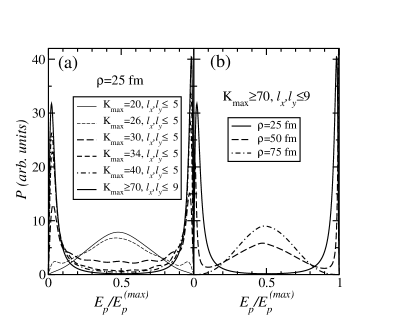
Figure 5: Proton energy distributions for the 3/2^- resonance in ¹⁷Ne where the maximum allowed emission energy is used as unit. The left part (a) is for $\rho$=25 fm for different values of $K_{max}$. The right part (b) is for a very large basis for increasing hyperradii. Only the lowest adiabatic effective potential is used.

V.4 Fragment energy distribution

After three-body decay of a given resonance, one of the most investigated observables is the energy distributions of the fragments after the decay. As shown in gar06 , these quantities are mainly determined from the properties of the coordinate space wave functions at large distances. This happens because the hyperspherical harmonics transform into themselves after Fourier transformation into momentum space. The kinetic energy distribution of the fragments at a given $\rho$ is therefore, except for a phase-space factor, obtained as the absolute square of the total wave function in coordinate space for that $\rho$, but where the five hyperangles are interpreted as in momentum space.

To obtain the energy distributions after decay one obviously needs to consider a value of $\rho$ clearly beyond the potential barrier, which means values of the hyperradius of several times the outer turning point. Following the discussion in the previous section, it is clear then that an accurate computation of such distributions requires a basis able to describe properly the three-body state at such large distance. In other words, reliable calculations require sufficiently large values of $K_{max}$, which will be larger than the ones reproducing the potential barrier up to the outer turning point.

For a system like ¹⁷Ne, where the outer turning point for the 3/2^- resonance is about 90 fm, the basis needed to compute the energy distributions after decay becomes soon very big, and therefore the numerical calculation very heavy. However, to illustrate the importance of a sufficient size of the basis, we first show in left part of Fig.5 the energy distribution of the proton when different $K_{max}$ values are used and when $\rho$ is fixed at 25 fm. For such $\rho$ value, as seen in Fig.4, accurate calculations are possible. Although this value of $\rho$ is clearly below the outer turning point, it illustrates the dependence of the energy distributions on the basis size. The only thing to have in mind is that the plotted distributions correspond to an intermediate stage, before the decay of the resonance. As a consequence, the plotted distributions do not necessarily resemble the experimental ones, which should be computed at a much larger value of $\rho$. The interplay between the two-body interactions can clearly change the energy distributions when moving from small to large values of $\rho$.

In any case, from Fig.4, we know that at $\rho$=25 fm a $K_{max}$ value of at least 40 is needed to have a converged potential at this distance. This fact is also reflected in left part of Fig.5, where we see that the energy distribution obtained when $K_{max}$=40 matches pretty well the result obtained with a much bigger basis (thick solid line). This energy distribution corresponds to a situation in which one of the protons takes most of the energy, while the other one stays close to the core. However, when the basis size decreases the proton energy distribution begins to fill the intermediate region, such that when $K_{max}$=20 (thin solid line) only one wide peak at about 0.5 is seen. The same strong dependence on $K_{max}$ as the one observed in the figure can be found for larger values of $\rho$, in particular for the values needed when computing the energy distributions after the decay.

To see the dependence on the hyperradius we show in the right part of Fig.5 how the proton energy distribution changes with the largest basis used in the left part. Now increasing $\rho$ shifts the proton energy distribution from two narrow peaks at low and high energy to one broad peak around half the maximum energy. These distributions have not yet converged as function of $\rho$. A larger value is needed with a correspondingly larger basis but the trend is clear. The protons are emitted roughly with equal energy. It is very illuminating to notice that the correctly converged result obtained for a large hyperradius and a large basis resembles an inaccurate result from a small basis and a much too small hyperradius.

VI Summary and conclusions

The partial width for a resonance decaying into three fragments must necessarily deal with the corresponding three-body problem. As for $\alpha$-emission we believe the crucial ingredients are provided by effective potentials at intermediate and large distances measured relative to the radius of the decaying nucleus. The many-body effects essentially only enter at small distances as preformation or spectroscopic factors and in microscopic derivations of the effective two-body interactions.

We concentrate in this paper on the three-body problem. We assume that the small distance boundary conditions necessary for resonance computations is simulated by the correct three-body energy and an attractive pocket within the confining barrier. We furthermore assume it is possible to specify the effective two and three-body interactions. With these assumptions we have isolated the crucial three-body problem from the underlying many-body degrees of freedom. Accurate resonance structures, partial decay widths, and fragment momentum distributions must first of all be computed for this well defined few-body problem. Inclusion of many-body effects may be important but this cannot avoid the three-body problem. The more elaborate schemes only add to the complexity involved in obtaining three-body input parameters.

We first formulate the basic concept of effective three-body potentials. As a test we then compare experimental widths for a number of ¹²C resonances with results from the simplest WKB application. As for $\alpha$-emission the largest variation is reproduced only leaving effects from preformation factors or equivalently many-body effects amounting to less than one to two orders of magnitude. The reproduced systematics is not monotonous with excitation energy or angular momentum.

The essence of the problem is now narrowed down to accurate computations of the effective three-body potentials. The classical turning points for the dominating potential therefore specify the region of interest in coordinate space. Any uncertainty in this region is enhanced exponentially in the computed widths. We give analytical estimates of both turning points and the number of contributing partial waves. We also estimate analytically, and demonstrate numerically, which basis size is necessary for accurate computations of the potentials in this coordinate region. Almost all published results employ insufficient basis sets.

We investigate the dependence of the computed widths on the effective two-body interactions. As for $\alpha$-emission the total energy is crucial and the two-body interactions should only provide roughly the same resonance energies independent of contributing spin and orbital angular momentum structure. The decisive properties are supplied by Coulomb and centrifugal forces. We discuss the different methods applied to width computations and conclude that they in most cases are equivalent.

Finally we illustrate how it is more difficult to get accurate momentum distributions of the fragments after three-body decay. These observables are sensitive to properties of the coordinate space wave functions at distances outside the turning point. Therefore an even larger basis is required. Unfortunately, a two-fold inaccurate computation with a too small basis and a too small hyperradius by a strange coincidence resembles the correctly converged result.

In conclusion, the partial three-body widths for decay of many-body resonances are first of all determined by three-body properties. Many-body effects are less important. The effective three-body potentials or equivalently the corresponding three-body wave functions are decisive and must be accurately computed.

References

- (1) G. Gamow, Z. Phys. 51, 204 (1928); 52, 510 (1928).
- (2) K.S. Krane, Introductory Nuclear Physics, John Wiley & Sons (1988) Page 254.
- (3) J. Al-Khalili and F. Nunes, J. Phys. G 29, R89 (2003).
- (4) J. P. Bondorf, A. S. Botvina, A. S. Iljinov, I. N. Mishustin, and K. Sneppen, Phys. Rep. 257, 133 (1995).
- (5) M. Thoennessen, Rep. Prog. Phys. 67, 1187 (2004).
- (6) B. Blank and M.J.G. Borge, Progr.Part.Nucl.Phys., 60, 403 (2008).
- (7) D.V. Fedorov, H.O.U. Fynbo, E.Garrido, and A.S. Jensen, Few-Body Systems 34, 33 (2004).
- (8) R. Álvarez-Rodríguez, A.S. Jensen, D.V. Fedorov, H.O.U. Fynbo, and E. Garrido, Phys.Rev.Lett. 99, 072503 (2007).
- (9) R. Álvarez-Rodríguez, E. Garrido, A.S. Jensen, D.V. Fedorov, and H.O.U. Fynbo, Eur. Phys. J. A 31, 303 (2007).
- (10) E. Garrido, D.V. Fedorov, and A.S. Jensen, Nucl. Phys. A 733, 85 (2004).
- (11) L.V. Grigorenko, R.C Johnson, I.G. Mukha, I.J. Thompson, and M.V. Zhukov, Phys. Rev. Lett. 85, 22 (2000).
- (12) J.R. Taylor Scattering Theory, Wiley and Sons, New York 1972, chapter 20.
- (13) H. Friedrich, Theoretical Atomic Physics, Springer-Verlag, Berlin Heidelberg 1991, chapter 4.
- (14) L.D. Landau and E.M. Lifshitz, Quantum mechanics, Pergamon Press, 1965, chapter XVII paragraph 134.
- (15) D.V. Fedorov and A.S. Jensen, Phys.Lett. B 389, 631 (1996).
- (16) R. Kamouni and D. Baye, Nucl.Phys. A 791, 68 (2007).
- (17) K. Arai, P. Descouvemont, D. Baye, W.N. Catford, Phys.Rev. C 68, 014310 (2003).
- (18) P. Descouvemont and A. Kharbach, Phys.Rev. C 63, 027001 (2001).
- (19) Y. Kanada-En’yo, Prog.Theor.Phys. 117, 655 (2007).
- (20) T. Neff and H. Feldmeier, Nucl.Phys. 738, 357 (2004).
- (21) J. Okolowicz, M. Ploszajczak, and I. Rotter, Phys. Rep. 374, 271 (2003).
- (22) N. Michel, W. Nazarewicz, M. Ploszajczak, and K. Bennaceur, Phys. Rev. Lett. 89, 042502 (2002).
- (23) R. Id Betan, R. J. Liotta, N. Sandulescu, and T. Vertse, Phys. Rev. Lett. 89, 042501 (2002).
- (24) K. Arai, Y. Ogawa, Y. Suzuki, K. Varga, Phys.Rev. C 54, 132 (1996).
- (25) A. Csoto, R.G. Lovas and A.T. Kruppa, Phys.Rev.Lett. 70, 1389 (1993); A. Csoto and G.M Hale, Phys.Rev.C 55, 536 (1997).
- (26) Y.K. Ho, Phys. Rep. 99, 1 (1983).
- (27) N. Tanaka, Y. Suzuki, K. Varga, and R.G. Lovas, Phys.Rev. C 59, 1391 (1999).
- (28) N. Tanaka, Y. Suzuki, and K. Varga, Phys.Rev. C 56, 562 (1997).
- (29) L.V. Grigorenko and M.V. Zhukov, Phys. Rev. C 76, 014008 (2007).
- (30) L.V. Grigorenko, I.G. Mukha, and M.V. Zhukov, Nucl. Phys. A 713, 372 (2003).
- (31) J.H. Macek, J.Phys., 1, 831 (1968).
- (32) E. Nielsen, D.V. Fedorov, A.S. Jensen and E. Garrido, Phys. Rep. 347, 373 (2001).
- (33) J.H. Macek, Few-Body Systems, 31, 241 (2002).
- (34) F. Ajzenberg-Selove, Nucl. Phys. A 560, 1 (1990), and http://www.tunl.duke.edu/nucldata/chain/12 newv.shtml.
- (35) E. Garrido, D.V. Fedorov, A.S. Jensen, and H.O.U. Fynbo, Nucl. Phys. A 748, 27 (2005).
- (36) A.S. Jensen, K. Riisager, D.V. Fedorov, and E. Garrido, Rev. Mod. Phys. 76, 215 (2004).
- (37) D.V. Fedorov, A. Cobis, and A.S. Jensen, Phys. Rev. C 59, 554 (1999).
- (38) E. Garrido, D.V. Fedorov, and A.S. Jensen, Nucl. Phys. A 708, 277 (2002).
- (39) T. Nakamura et al., Phys. Rev. Lett. 96, 252502 (2006).
- (40) E. Garrido, D.V. Fedorov, and A.S. Jensen, Phys. Rev. C 68, 014002 (2003).
- (41) C. Kurokawa and K. Kato, Nucl.Phys. A 792 (2007) 87; Phys. Rev. C 71, 021301(R) (2005).
- (42) H. Masui, K. Kato, and K. Ikeda, Phys. Rev. C 75, 034316 (2007).
- (43) C. Aa. Diget et al., Nucl. Phys. A 760, 3 (2005).
- (44) L.V. Grigorenko, R.C. Johnson, I.G. Mukha, I.J. Thompson, and M.V. Zhukov, Phys. Rev. C 64, 054002 (2001).
- (45) E. Garrido, D.V. Fedorov, A.S. Jensen, and H.O.U. Fynbo, Nucl. Phys. A 790, 96 (2007).
- (46) E. Garrido, D.V. Fedorov, A.S. Jensen, and H.O.U. Fynbo, Nucl. Phys. A 766, 74 (2002).