Driven quantum coarsening

Abstract

We study the driven dynamics of quantum coarsening. We analyze models of $M$-component rotors coupled to two electronic reservoirs at different chemical potentials that generate a current threading through the system. In the large $M$ limit we derive the dynamical phase diagram as a function of temperature, strength of quantum fluctuations, voltage and coupling to the leads. We show that the slow relaxation in the ordering phase is universal. On large time and length scales the dynamics are analogous to stochastic classical ones, even for the quantum system driven out of equilibrium at zero temperature. We argue that our results apply to generic driven quantum coarsening.

Phase transitions are central to condensed matter and statistical physics. Initially, emphasis was put on classical and quantum equilibrium phase transitions. Later, attention moved to non-equilibrium phase transitions in which quantum fluctuations can be neglected. These are realized when a system is forced in a non equilibrium steady state (by a shear rate, an external current flowing through it, etc.) OnukiKawasaki ; DombGreen or when it just fails to relax (e.g. after a quench) and displays aging phenomena Struick ; LeticiaLesHouches . The study of steady states in small quantum systems driven out of equilibrium MitraMillisReichman has been recently boosted by their relevance for nano-devices. In contrast, the effect of a drive on a macroscopic system close to a quantum phase transition is a rather unexplored subject. Some works have focused on non-linear transport properties close to an (equilibrium) quantum phase transition DalidovichPhillips ; GreenSondhi ; HoganGreen . Others have studied how the critical properties are affected by a drive MitraKimMillis ; Feldman ; MitraMillis . However, a global understanding of phase transitions in the parameter space $T$ (temperature), $V$ (drive), $\Gamma$ (strength of quantum fluctuations), and the rôle played by the environment, is still lacking. Furthermore, experiments in $2d$ electronic systems Ovadyahu ; Popovic show interesting features in the relaxation toward the quantum non-equilibrium steady state (QNESS) but these have not been addressed theoretically yet (except for mueller ).

A number of intriguing questions arise in the context of driven quantum phase transitions, some of which are: How long does it take to reach the QNESS after one of the parameters $T,\ V,\ \Gamma$ is changed? Do the systems always relax to the QNESS or, as for classical systems, do quenches deep in the $T,\ V,\ \Gamma$ phase diagram lead to aging phenomena and glassy dynamics? What are the properties of the latter ‘doubly non-equilibrium’ dynamics? Are quantum quenches, obtained by changing $V$ and $\Gamma$ at $T=0$, different from their classical counterpart?

$\scriptstyle\Gamma_{c}(V=0)$	$\scriptstyle\sim$	$\scriptstyle\overline{T}_{c}-T$
$\scriptstyle\Gamma_{c}(T=0)$	$\scriptstyle\sim$	$\scriptstyle{\rm NA}$
$\scriptstyle T_{c}(\Gamma=0)$	$\scriptstyle\sim$	$\scriptstyle{\rm NA}$
$\scriptstyle T_{c}(V=0)$	$\scriptstyle\sim$	$\scriptstyle\left(\overline{\Gamma}_{c}-\Gamma\right)^{1/2}$
$\scriptstyle V_{c}(T=0)$	$\scriptstyle\sim$	$\scriptstyle\left(\overline{\Gamma}_{c}-\Gamma\right)^{1/2}$
$\scriptstyle V_{c}(\Gamma=0)$	$\scriptstyle\sim$	$\scriptstyle\left(\overline{T}_{c}-T\right)^{1/2}$

Figure 1: Non-equilibrium phase diagram for reservoirs with a much larger bandwidth than all other energy scales ($\hbar\omega_{F}\gg J$). Close to the critical point $\overline{V}_{c}=V_{c}(T=\Gamma=0)$ the critical lines are non-analytical (${\rm NA}$). Close to $\overline{T}_{c}$ and $\overline{\Gamma}_{c}$ they are power laws with exponents given next to the figure. The arrow above $\Gamma_{c}$ indicates that the critical surface is pulled up by increasing the coupling to the leads.

The aim of this work is to answer these questions for a class of analytically tractable models, systems of $M-$component quantum rotors that encompass an infinite range spin-glass and its 3d pure counterpart modeling coarsening phenomena. Models of quantum rotors are non-trivial but still relatively simple and provide a coarse-grained description of physical systems such as Bose-Hubbard models and double layer antiferromagnets SachdevBook . The out of equilibrium drive is provided by two external electron reservoirs that induce a current flowing through the system. In the simplest setting MitraKimMillis each rotor is coupled to two independent reservoirs. Using the Schwinger-Keldysh formalism we analyze the out of equilibrium dynamics in the large $M$ limit. We find a phase transition, see Fig. 1, between a QNESS ($V\neq 0$) and an ordered phase, we study its critical properties and we discuss the effect of the environment.

The model we focus on is an infinite-range quantum disordered system made of $N$ $M$-component rotors interacting via random Gaussian distributed couplings, $J_{ij}$, with zero mean and variance $J^{2}/N$. Its Hamiltonian is

$$H_{S}=\frac{\Gamma}{2\hbar^{2}M}\sum_{i=1}^{N}\mathbf{L}_{i}^{2}-\sum_{i<j}J_{ij}\mathbf{n}_{i}\mathbf{n}_{j}\;,\;\;\;\mathbf{n}_{i}^{2}=M\;\;\forall i\;.$$ (1)

$n_{i}^{\mu}$ are the $M$ components of the $i$-th rotor and $L_{i}^{\mu\nu}=n_{i}^{\mu}p_{i}^{\nu}-n_{i}^{\nu}p_{i}^{\mu}$, with $p_{i}^{\mu}=-i\hbar\partial/\partial n_{i}^{\mu}$, are the $M(M-1)$ components of the $i$-th generalized angular momentum operator with $\mathbf{L}_{i}^{2}=\sum_{\mu<\nu}(L_{i}^{\mu\nu})^{2}$ SachdevBook ; SachdevYe . $\Gamma$ controls the strength of quantum fluctuations; as $\Gamma\to 0$ the model approaches the classical $M$-component Heisenberg fully-connected spin-glass. In the large $M$ limit it is equivalent to the quantum fully-connected $p=2$ spherical spin-glass Cude ; Rokni . A mapping to ferromagnetic coarsening in the $3d$ O(${\cal N}$) model can be established in the classical and large ${\cal N}$ limits LeticiaLesHouches . As we shall show, this mapping holds for the quantum model as well. Thus, it allows us to extend our results also to the 3d ferromagnetic model in the large $M$ limit.

The system is coupled to two independent and non-interacting ‘left’ ($L$) and ‘right’ ($R$) electronic reservoirs in equilibrium at different chemical potentials $\mu_{L}=\mu$ and $\mu_{R}=\mu+eV$ and the same temperature $T$. $R$ and $L$ reservoirs act as source and drain, respectively. The details of their Hamiltonian are not important since in the small spin-bath coupling we concentrate on only the electronic Green functions matter. We focus on free electrons with the same symmetric density of states, $\rho_{L}(\epsilon)=\rho_{R}(\epsilon)=\rho(\epsilon)$, centered at $\epsilon=0$, and with typical variation scale around $\hbar\omega_{F}$ .

Each rotor is coupled non-linearly to its (double) electron bath. For example, for $M=3$ rotors we take $H_{SB}=\frac{1}{{\cal M}}\sum_{i\alpha ll^{\prime}\gamma\gamma^{\prime}}\hbar\omega_{\gamma\gamma^{\prime}}n_{i}^{\alpha}\;[c^{\dagger}_{liL\gamma}\frac{\sigma_{ll^{\prime}}^{\alpha}}{2}c_{l^{\prime}iR\gamma}+L\leftrightarrow R]$ where $c^{\dagger}_{liR(L)\gamma},\ c_{liR(L)\gamma}$ are the fermionic operators of the $R(L)$ reservoirs, $\hbar\omega_{\gamma\gamma^{\prime}}$ is the electron-bath coupling, chosen to be constant: $\hbar\omega_{\gamma\gamma^{\prime}}=\hbar\omega_{c}$. $\mathbf{\sigma}^{\alpha}$ are the Pauli matrices ($\alpha=1,...,M$). $\gamma=1,...,\cal M$ is the fermion label inside the reservoirs.

System and reservoirs are uncoupled at time $t<0$ and evolve with $H=H_{S}+H_{B}+H_{SB}$ at $t>0$. The density matrix at $t=0$, $\varrho=\varrho_{S}\otimes\varrho_{L}\otimes\varrho_{R}$, provides the initial condition. $\varrho_{S}$, $\varrho_{L}$ and $\varrho_{R}$ correspond to equilibrium of the system at temperature $T_{0}\gg 1$, and the $L$ and $R$ reservoirs at temperature $T$ and chemical potentials $\mu$ and $\mu+eV$, respectively. For simplicity, $\varrho_{S}$ is taken to be the identity; this choice is equivalent to any other one uncorrelated with disorder Culo .

We analyze the $t>0$ dynamics by using the Schwinger-Keldysh formalism yielding a functional-integral representation of the Heisenberg evolution SchwingerKeldysh ; Culo ; preparation . Each field carries a $\pm$ index associated to the forward and backward evolution. The action corresponding to Eq. (1) is

$$S_{S}=\sum_{a=\pm}a\int{\rm d}t\left[\frac{\hbar^{2}}{2\Gamma}\sum_{i}(\mathbf{\dot{n}}_{ia})^{2}+\sum_{i<j}J_{ij}\mathbf{n}_{ia}\mathbf{n}_{ja}\right]\;.$$

The path-integral runs over paths such that $\mathbf{n}_{ia}^{2}(t)=M,\ \forall iat$. One may lift this constraint by using the integral representation of the Dirac delta. This amounts to introducing auxiliary imaginary fields $\lambda_{ia}(t)$ and adding $S_{\lambda}=\sum_{a=\pm}\frac{a}{2}\int{\rm d}t\sum_{i}\lambda_{ia}(t)(\mathbf{n}_{ia}^{2}(t)-M)$ to the action.
After expanding the system-leads interaction up to second order in $g\equiv\omega_{c}/\omega_{F}$, integrating out the fermionic fields, and taking the large $M$ limit we obtain a (Feynman-Vernon-like) action for the rotors. The detailed computation preparation confirms that several system-reservoir coupling that preserve the $O(M)$ symmetry and the addition of different $LL$ and $RR$ couplings do not modify our results qualitatively. In short we obtain

$$S_{SB}=-\frac{1}{2}\sum_{ab=\pm}\int{\rm d}t{\rm d}t^{\prime}\ \Sigma_{ab}^{B}(t,t^{\prime})\ \sum_{i}\mathbf{n}_{ia}(t)\mathbf{n}_{ib}(t^{\prime})\;,$$

$$\Sigma_{ab}^{B}(t,t^{\prime})=-iab\hbar\omega_{c}^{2}\left[G^{R}_{ab}(t,t^{\prime})G^{L}_{ba}(t^{\prime},t)+L\leftrightarrow R\right]\;.$$

The electronic Green functions are $G_{ab}(t,t^{\prime})\equiv-i\langle{\cal T}\psi_{a}(t)\psi^{\dagger}_{b}(t^{\prime})\rangle$ with $\psi_{a}(t),\psi^{\dagger}_{a}(t)$ the fermionic fields and ${\cal T}$ the time-ordering operator on the closed contour. It is convenient to change basis and use retarded, $G_{R}^{B}=(G_{+-}^{B}-G_{++}^{B})/\hbar$, advanced, $G_{A}^{B}=(G_{-+}^{B}-G_{++}^{B})/\hbar$, and Keldysh, $G_{K}^{B}=i(G_{++}^{B}+G_{--}^{B})/2$, Green functions. The $\Sigma$’s transform in a similar way. For identical reservoirs at temperature $T$ and chemical potential $\mu$ ($V=0$), the self-energy components verify the usual fluctuation dissipation relation of a standard bosonic bath $\Sigma_{K}^{B}(\omega)=\hbar\coth(\beta\hbar\omega/2)\Im\Sigma_{R}^{B}(\omega)$, with $\beta=1/T$ and $k_{B}=1$.

Collecting all contributions the total action, $S=S_{S}+S_{\lambda}+S_{SB}$, is $O(MN)$. Given that the zero-source generating functional equals one, one can simply compute its average over quenched randomness Culo and use a saddle-point evaluation of the resulting path-integral that is exact in the large $M$ and $N$ limits. The value of $\lambda_{ia}(t)$ at the saddle point is a spatially homogenous function $\lambda(t)$. Its time-dependence is determined by the condition $\langle\mathbf{n}_{ia}^{2}(t)\rangle=M$ with the average taken over $S$ preparation .

The macroscopic dynamic order parameters are the symmetric two-time correlation and instantaneous linear response that in the operator formalism are defined as $MC(t,t_{w})\equiv\langle\{{\bf n}_{i}(t),{\bf n}_{i}(t_{w})\}/2\rangle$ and $MR(t,t_{w})\equiv\delta\langle{\bf n}_{i}(t)\rangle/\delta{\bf h}_{i}(t_{w})|_{h=0}=-1/\hbar\langle[{\bf n}_{i}(t),{\bf n}_{i}(t_{w})]\rangle\theta(t-t_{w})$. The field ${\bf h}_{i}$ couples linearly to the $i$-th rotor and the last identity is the Kubo formula valid in linear response. The exact Schwinger-Dyson equations then read:

$${\cal D}(t)R(t,t_{w})=\delta(t-t_{w})+\int_{t_{w}}^{t}{\rm d}t^{\prime\prime}\ \Sigma_{R}(t,t^{\prime\prime})R(t^{\prime\prime},t_{w})\;,$$

$${\cal D}(t)C(t,t_{w})=\int_{0}^{t}{\rm d}t^{\prime\prime}\ \Sigma_{R}(t,t^{\prime\prime})C(t^{\prime\prime},t_{w})$$

$$\qquad\qquad\qquad\;\;\;+\int_{0}^{t_{w}}{\rm d}t^{\prime\prime}\ \Sigma_{K}(t,t^{\prime\prime})R(t_{w},t^{\prime\prime})\;,$$ (2)

with ${\cal D}(t)=\hbar^{2}\Gamma^{-1}\partial_{t}^{2}+\lambda(t)$, the retarded and Keldysh self-energies given by $\Sigma_{R}=\Sigma_{R}^{B}+J^{2}R$ and $\Sigma_{K}=\Sigma_{K}^{B}+$$J^{2}C$, and $\lambda(t)=-\hbar^{2}\Gamma^{-1}\partial^{2}_{t^{2}}C(t,t_{w}\to t^{-})+$$\int_{0}^{t}{\rm d}t^{\prime\prime}\;[\Sigma_{R}(t,t^{\prime\prime})C(t,t^{\prime\prime})+$$\Sigma_{K}(t,t^{\prime\prime})R(t,t^{\prime\prime})]$.

In the QNESS, the dynamics are stationary but they do not satisfy the fluctuation-dissipation theorem (FDT) when $V\neq 0$. The Lagrange multiplier approaches a constant, $\lambda(t)\to\lambda_{\infty}$, and the linear response satisfies a closed equation that once Fourier transformed reads $R(\omega)=-[\hbar^{2}\Gamma^{-1}\omega^{2}-\lambda_{\infty}+\Sigma_{R}^{B}(\omega)+J^{2}R(\omega)]^{-1}$. The physical solution to this quadratic equation is the one that satisfies $R(\omega\to\infty)=0$. The correlation is given by $C(\omega)=\Sigma_{K}(\omega)|R(\omega)|^{2}$ and the spherical constraint, $C(t,t)=1$, implies

$$\int_{0}^{\infty}\frac{{\rm d}\omega}{2\pi}\;\frac{\Sigma_{K}^{B}(\omega)}{\Im\Sigma_{R}^{B}(\omega)}\;\Im R(\omega)=1/2\;.$$ (3)

The phase transition occurs when $R(\omega=0)=\int{\rm d}tR(t)$ ceases to be real, indicating that the stationary condition necessary to Fourier transform is no longer valid. Concomitantly, the derivatives of $R(\omega)$ in $\omega=0$ diverge and hence the real-time response function shows a power law decay. This happens when $\lambda_{\infty}=\lambda_{c}=2J+\Sigma_{R}^{B}(\omega=0)$. Inserting $\lambda_{c}$ in Eq. (3), we then obtain the equation for the critical manifold in the $T,V,\Gamma$ space (for a given $g$ and $\hbar\omega_{F}$). We shall derive the critical manifold for different reservoirs in full detail in preparation ; we summarize here some of the salient features.

We first consider $g\to 0$ after the long-time limit such that the asymptotic regime has been established and we take $\hbar\omega_{F}$ much larger than any other energy scale. For $\Gamma=V=0$ we recover the classical critical temperature, $\overline{T}_{c}=J$ SachdevYe ; Cude . At $V=T=0$ we obtain $\overline{\Gamma}_{c}=(3\pi/4)^{2}J$, as for the $p=2$ quantum spherical model in equilibrium SachdevYe and its dynamics coupled to an equilibrium oscillator bath Rokni . Finally, the critical point $\overline{V}_{c}$ on the $\Gamma=T=0$ line is determined by

$$\int_{\mu}^{\mu+e\overline{V}_{c}}{\rm d}\epsilon\;\left[\frac{\rho_{L}(\epsilon)}{2J}-\dot{\rho}_{L}(\epsilon)\right]\rho_{R}(\epsilon)=\rho_{L}\left(\mu\right)\rho_{R}\left(\mu\right)$$

that can be solved numerically and also analytically in some special cases. In the large bandwidth limit $\hbar\omega_{F}\gg J$ and we find $e\overline{V}_{c}=2J$ for the $\rho_{L}=\rho_{R}=\rho$ symmetric case, with $\mu=0$ and differentiable at the origin. The form of the critical lines are shown in Fig. 1.

As for finite $\hbar\omega_{F}$ we find that $\overline{V}_{c}$ varies (contrary to $\overline{T}_{c}$ and $\overline{\Gamma}_{c}$) upon decreasing $\hbar\omega_{F}/J$, the critical line $V_{c}(T,\Gamma=0)$ is re-entrant and, for a single band, $eV$ is bounded when the $R$ reservoir is filled.

When the coupling to the electronic reservoirs, $g$, is finite the critical line in the $\Gamma=0$ plane remains unaltered but the critical surface on the $\Gamma$ direction is pulled ‘upwards’ enlarging the low temperature phase for increasing values of $g$. This is similar to what was found for quantum oscillator Ohmic baths and is due to a spin-localization-like effect effect-bath ; Rokni .

   

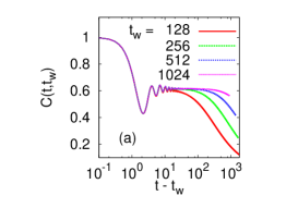
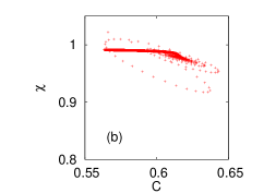
Figure 2: Dynamics in the driven coarsening regime: numerical solution to Eqs. (2) after a quench to $T=0.2J,V=0.2J$, $\Gamma=1$, $g=1$ with $\hbar\omega_{F}=10J$. (a) The symmetric correlation $C(t,t_{w})$. (b) The integrated linear response, $\chi(t,t_{w})=\int_{t_{w}}^{t}{\rm d}t^{\prime}R(t,t^{\prime})$ against $C$, for $t_{w}=1024$ and using $t$ as a parameter. The curved part corresponds to the stationary and oscillatory regime with $(t-t_{w})/t_{w}\to 0$ while the straight line is for times in the monotonic aging decay of $C$.

We now turn to the dynamics. Our numerical and analytical analysis of Eqs. (2) show that after a quench in the low-$T$, weak-$\Gamma$ and weak-$V$ phase, the dynamics do not reach a QNESS preparation . There is a separation of two-time scales typical of aging phenomena LeticiaLesHouches . First, a stationary regime for short time differences $t-t_{w}$ with respect to the waiting-time after the quench, $t_{w}$, in which the symmetric correlation approaches a plateau asymptotically in the time-difference. Later, an aging regime in which $C$ depends on the two times explicitly. This behavior is shown in Fig. 2(a). The plateau value $q_{\rm EA}$, so-called Edwards-Anderson parameter, measures the fraction of frozen rotor fluctuations on timescales much smaller than $t_{w}$. The stationary decay depends on all control parameters. $q_{\rm EA}$ approaches one at $T=\Gamma=V=0$ and zero on the critical manifold as in a second order transition. In the aging regime, the correlation normalized by $q_{\rm EA}$ is identical to the classical one Cude :

$$C(t,t_{w})/q_{\rm EA}\simeq 2\sqrt{2}\ (t_{w}/t)^{3/4}\ (1+t_{w}/t)^{-3/2}$$ (4)

for $0<t/t_{w}<1$. We shall prove this result and unveil the connection with coarsening anticipated previously by exploiting the quadradic form of the full action in the ${\bf n}$ fields. Under the Keldysh rotation $({\bf n}^{+},{\bf n}^{-})\to(i\hat{\bf n},{\bf n})$ with $i\hat{\bf n}\equiv i({\bf n}^{+}-{\bf n}^{-})/\hbar$ and ${\bf n}\equiv({\bf n}^{+}+{\bf n}^{-})/2$ the action is identical to the Martin-Siggia-Rose one for a classical Langevin process in a harmonic potential $\sum_{ij}(J_{ij}-\lambda(t)\delta_{ij}){\bf n}_{i}\cdot{\bf n}_{j}$. The noise statistics is, however, peculiar: because of the quantum origin of the environment it has memory, depends on $\hbar$ and satisfies the quantum FDT in the $V=0$ case. The Langevin equations are rendered independent – apart from a residual coupling through the Lagrange multiplier – by a rotation onto the basis that diagonalizes the interaction matrix $J_{ij}$: ${\bf n}_{\mu}=\sum_{j}v_{\mu}^{j}{\bf n}_{j}$ and $i\hat{\bf n}_{\mu}=\sum_{j}v^{j}_{\mu}i\hat{\bf n}_{j}$ with $v^{j}_{\mu}$ the eigenvector associated to the eigenvalue $J_{\mu}$. The analysis then follows the same route as in Cude , see preparation . One finds quite naturally that the long-time dynamics correspond to a Bose-Einstein-like condensation process of the $M$ $N$-dimensional ‘vectors’ ${\bf n}_{i}$ on the direction of the edge eigenvector. The relaxation is then controlled by the decay of $\rho(J_{\mu})$ close to its edge. For Gaussian i.i.d. couplings $\rho(J_{\mu})\propto(2J-J_{\mu})^{1/2}$. This coincides with the distribution of the modulus of the Laplacian eigenvalues, $dk^{2}k^{2(d/2-1)}=dk^{2}k^{2\times 1/2}$ in $d=3$. For this reason all models with a square root singularity of the distribution of ‘masses’ $J_{\mu}$, as the ferromagnetic rotor model in $d=3$ and the completely connected spin glass rotor model, are characterized by the same long-time dynamics. Now let us show that the aging dynamics are indeed equivalent to their classical counterpart. In the ordered phase, taking the long $t_{w}$ and $t-t_{w}$ limits with $t/t_{w}$ fixed (low frequency aging regime) the second-time derivatives in the effective Langevin equations can be neglected. Furthermore, only the low-frequency ($\omega\ll 1/{\beta\hbar}$) behavior of the kernels plays a rôle in this regime. In this $\omega\rightarrow 0$ limit, $\Sigma_{K}^{B}(\omega)\to\ \mbox{ct}\in\Re$, and $\Sigma_{R}(\omega)$ is linear. Therefore the noise kernels approach a classical Ohmic white-noise limit with ‘temperature’

$$T^{*}=\lim_{\omega\rightarrow 0}\Sigma_{K}^{B}(\omega)/[2\partial_{\omega}\Im\Sigma_{R}^{B}(\omega)]\;.$$ (5)

At $V=0$ one gets $T^{*}=T$. Instead, at $T=0$ and $eV\ll\hbar\omega_{F}$, one has $T^{*}=eV/2$: the voltage plays the rôle of a bath temperature. This fact has already been reported and it is at the root of the derivation of the stochastic Gilbert equation for a spin under bias Gilbert . Having argued that the long-time dynamics is governed by a classical Langevin equation at temperature $T^{*}$, it is justified that the correlation scales as the one in Cude for $t/t_{w}=O(1)$, see Eq. (4), a result with two interesting consequences. In the case of (large $M$) quantum $3d$ coarsening the classical-quantum mapping extends to space-time correlations preparation and proves the existence of a growing coherence length $\xi(t_{w})\propto t_{w}^{1/2}$ over which the rotors are oriented in the same direction and provides a real-space interpretation of aging. Moreover, in the same long-time regime, the linear response also scales as in the classical problem. Therefore, the quantum fluctuation-dissipation relation between integrated linear-response, $\chi$, and symmetric correlation approaches the classical one, $\chi\sim\mbox{ct}+(q_{\rm EA}-C)/T_{\rm eff}$, with an infinite effective temperature Cukupe , $T_{\rm eff}\to\infty$, as shown in Fig. 2(b) (see also Culo ; other-quantum ). In short, the asymptotic aging dynamics are universal, in the sense that the scaling functions do not depend on $T,\Gamma,V$ in the coarsening phase and, hence, are equivalent to the classical un-driven ones ($\Gamma=V=0$) Cukulepe . This result mirrors the one obtained in MitraKimMillis for steady state dynamics.

The environment plays a dual rôle: its quantum character basically determines the phase diagram but the coarsening process at long times and large length-scales only ‘feels’ a classical white bath at temperature $T^{*}$. The two-time dependent decoherence phenomenon (absence of oscillations, validity of a classical FDT when $t/t_{w}=O(1)$, etc.) is intimately related to the development of a non-zero (actually infinite) effective temperature, $T_{\rm eff}$, of the system as defined from the deviation from the (quantum) FDT Cukupe . $T_{\rm eff}$ should be distinguished from $T^{*}$ as the former is generated not only by the environment but by the system interactions as well ($T_{\rm eff}>0$ even at $T^{*}=0$ Culo ; other-quantum ). Moreover, we found an extension of the irrelevance of $T$ in classical ferromagnetic coarsening ($T=0$ ‘fixed-point’ scenario): after a suitable normalization of the observables that takes into account all microscopic fluctuations (e.g. $q_{\rm EA}$) the scaling functions are independent of all parameters including $V$ and $\Gamma$. Although we proved this result through a mapping to a Langevin equation that applies to quadratic models only, we expect it to hold in all instances with the same type of ordered phase, say ferromagnetic, and a long-time aging dynamics dominated by the slow motion of large domains. Thus, a large class of coarsening systems (classical, quantum, pure and disordered) should be characterized by the same scaling functions. It could be worth studying carefully systems evolving by barrier crossing, a rapid process in which not only the low frequency behavior of the bath may be relevant.

We thank C. Chamon, L. Chaput, A. Millis and A. Mitra for useful discussions. LFC is a member of IUF.

References

- (1) A. Onuki and K. Kawasaki, Ann. Phys. (N.Y.) 121, 456 (1979).
- (2) B. Schmittmann and R. K. P. Zia, Vol. 17 of Phase Transitions and Critical Phenomena, eds. C. Domb and J. L. Lebowitz (Academic Press, London, 1995).
- (3) L. C. E. Struick, Physical Aging in Amorphous Polymers and Other Materials, (Elsevier, Amsterdam, 1978).
- (4) L. F. Cugliandolo, in Les Houches Session 77, J-L. Barrat et al eds. (Springer-EDP Sciences, 2002), arXiv:cond-mat/0210312. G. Biroli, J. Stat. Mech. P05014 (2005).
- (5) L. Arrachea and L. F. Cugliandolo, Europhys. Lett. 70, 642 (2005). D. Segal et al, Phys. Rev. B 76, 195316 (2007) and refs therein.
- (6) D. Dalidovich and P. Phillips, Phys. Rev. Lett. 93, 027004 (2004).
- (7) A. G. Green and S. L. Sondhi, Phys. Rev. Lett. 95, 267001 (2005).
- (8) P. M. Hogan and A. G. Green, arXiv:cond-mat/0607522.
- (9) A. Mitra et al, Phys. Rev. Lett. 97, 236808 (2006).
- (10) D. E. Feldman, Phys. Rev. Lett. 95, 177201 (2005).
- (11) A. Mitra and A. J. Millis, arXiv:0804.3980
- (12) Z. Ovadyahu, Phys. Rev. B 73, 214204 (2006).
- (13) D. Popovic et al. Proceedings of SPIE, 5112, 99 (2003).
- (14) E. Lebanon, M. Müeller, Phys. Rev. B 72, 174202 (2005).
- (15) S. Sachdev, Quantum Phase Transitions, (Cambridge Univ. Press, 1999).
- (16) J. Ye, S. Sachdev, and N. Read, Phys. Rev. Lett. 70, 4011 (1993). T. K. Kopeć, Phys. Rev. B 50, 9963 (1994).
- (17) L. F. Cugliandolo and D. S. Dean, J. Phys. A 28, 4213 (1995).
- (18) M. Rokni and P. Chandra, Phys. Rev. B 69, 094403 (2004).
- (19) L. F. Cugliandolo and G. S. Lozano, Phys. Rev. Lett. 80, 4979 (1998); Phys. Rev. B 59, 915 (1999).
- (20) U. Weiss, Quantum dissipative systems (World Scientific, Singapore, 1993). A. Kamenev, in Les Houches Session 81, H. Bouchiat et al. eds. (Springer-EDP Sciences, 2004), arXiv:cond-mat/0412296.
- (21) C. Aron, G. Biroli, and L. F. Cugliandolo, in preparation.
- (22) L. F. Cugliandolo et al, Phys. Rev. B 66, 014444 (2002).
- (23) A. S. Núñez and R. A. Duine, Phys. Rev. E 77, 054401 (2008).
- (24) M. P. Kennett and C. Chamon, Phys. Rev. Lett. 86, 1622 (2001). G. Biroli and O. Parcollet, Phys. Rev. B 65, 094414 (2002).
- (25) L. F. Cugliandolo et al, Phys. Rev. E 55, 3898 (1997).
- (26) Coarsening survives at finite under the current as opposed to the fact that aging is killed by a shear rate in the classical limit, see L. F. Cugliandolo et al, Phys. Rev. Lett. 78, 350 (1997) and L. Berthier et al Phys. Rev. E 61, 5464 (2000). We attribute the difference to the fact that in the quantum model while the one can associate to shear diverges preparation .