The Chemical Abundances of Tycho G in Supernova Remnant 1572

Abstract

We present an analysis of the chemical abundances of the star Tycho G in the direction of the remnant of supernova (SN) 1572, based on Keck high-resolution optical spectra. The stellar parameters of this star are found to be those of a G-type subgiant with $T_{\mathrm{eff}}=5900\pm 100$ K, $\log(g/{\rm cm~{}s}2)$ $=3.85\pm 0.30$ dex, and $\mathrm{[Fe/H]}=-0.05\pm 0.09$. This determination agrees with the stellar parameters derived for the star in a previous survey for the possible companion star of SN 1572 (Ruiz-Lapuente et al. 2004). The chemical abundances follow the Galactic trends, except for Ni, which is overabundant relative to Fe, $[{\rm Ni/Fe}]$ $=$ 0.16 $\pm$ 0.04. Co is slightly overabundant (at a low significance level). These enhancements in Fe-peak elements could have originated from pollution by the supernova ejecta. We find a surprisingly high Li abundance for a star that has evolved away from the main sequence. We discuss these findings in the context of companion stars of supernovae.

1 Introduction

Type Ia supernovae (SNe Ia) are the best known cosmological distance indicators at high redshifts. Their use led to the discovery of the currently accelerating expansion of the Universe (Riess et al. 1998; Perlmutter et al. 1999); see Filippenko (2005) for a review. They were also used to reveal an early era of deceleration, up through about 9 billion years after the big bang (Riess et al. 2004, 2007). Larger, higher-quality samples of SNe Ia, together with other data, are now providing increasingly accurate and precise measurements of the dark energy equation-of-state parameter, $w=P/(\rho c2)$ (e.g., Astier et al. 2006; Riess et al. 2007; Wood-Vasey et al. 2007; Kowalski et al. 2008).

Though the increase in the empirical knowledge of SNe Ia has led to an enormous advance in their cosmological use, the understanding of the explosion mechanism still requires careful evaluation (e.g., Hillebrandt & Niemeyer 2000; Wheeler 2007). While in Type II SNe we have the advantage that the explosion leaves a compact star to which surviving companions (if they exist) often remain bound, thus enabling a large number of studies (e.g., Martín et al. 1992; Israelian et al. 1999), in SNe Ia the explosion almost certainly does not produce any compact object.

To investigate how the explosion takes place, we examine the rates of SNe Ia at high redshifts, or we can take a more direct approach and survey the field of historical SNe Ia. The latter strategy has been followed since 1997 in a collaboration that used the observatories at La Palma, Lick, and Keck (Ruiz-Lapuente et al. 2004). The stars appearing within the 15$\%$ innermost area of the remnant of SN 1572 ($0.65^{\prime}$) were observed both photometrically and spectroscopically at multiple epochs over seven years. The proper motions of these stars were measured as well using images obtained with the WFPC2 on board the Hubble Space Telescope (HST) (GO–9729). The results revealed that many properties of any surviving companion star of SN 1572 were unlike those predicted by hydrodynamical models. For example, the surviving companion star (if present) could not be an overluminous object nor a blue star, as there were none in that field. Red giants and He stars were also discarded as possible companions.

A subgiant star (G2 IV) with metallicity close to solar and moving at high speed for its distance was suggested as the likely surviving companion of the exploding white dwarf (WD) that produced SN 1572 (Ruiz-Lapuente et al. 2004). This star, denoted Tycho G, has coordinates $\alpha=00^{\rm h}25^{\rm m}23.7^{\rm s}$ and $\delta=+64^{\circ}08^{\prime}02^{\prime\prime}$ (J2000.0). Comparisons with a Galactic model showed that the probability of finding a rapidly moving subgiant with solar metallicity at a location compatible with the distance of SN 1572 was very low. A viable scenario for the Tycho SN 1572 progenitor would be a system resembling the recurrent nova U Scorpii. This system contains a white dwarf of $M_{\rm WD}=1.55\pm 0.24$ M${}_{\odot}\;$and a secondary star with $M_{2}=0.88\pm 0.17$ M${}_{\odot}\;$orbiting with a period $P_{\rm orb}\approx 1.23$ d (Thoroughgood et al. 2001).

On the other hand, based on analysis of low-resolution spectra, Ihara et al. (2007) recently claimed that the spectral type of Tycho G is not G2 IV as found by Ruiz-Lapuente et al. (2004), but rather F8 V. In addition, Ihara et al. (2007) suggested the star Tycho E as the companion star of the Tycho SN 1572, but we consider their conclusion to be unjustified. They base it on a single Fe I feature at 3720 Å in a spectrum having a signal-to-noise ratio (SNR) of only $\sim 13$. The short spectral range of their data (3600–4200 Å) and the low resolution ($\lambda/\Delta\lambda\approx 400$, with a dispersion of 5 Å/pixel) add to our concern.

The present work resolves questions regarding the metallicity and spectral classification of Tycho G. We concentrate on providing both the chemical composition of the star and the stellar parameters as derived from new data. In addition, we present a detailed chemical analysis of Tycho G aimed at examining the possible pollution of the companion star by the supernova. Although more data are still required to definitively settle this issue, the overall properties of this star remain consistent with being the surviving companion of SN 1572.

2 Observations

In order to perform an abundance analysis of Tycho G, spectra of it were obtained with the High Resolution Echelle Spectrometer (HIRES; Vogt et al. 1994) on the Keck I 10-m telescope (Mauna Kea, Hawaii). Nine spectra (with individual exposure times of 1200 s and 1800 s) were obtained on 10 September 2006 (UT dates are used throughout this paper) and four spectra (with exposure times of 1800 s) on 11 October 2006, covering the spectral regions 3930–5330 Å, 5380–6920 Å, and 6980–8560 Å at resolving power $\lambda/\Delta\lambda\approx 50,000$.

The spectra were reduced in a standard manner using the makee package. We checked in each individual spectrum the accuracy of the wavelength calibration using the [O I] $\lambda$6300.3 and $\lambda$5577.4 night-sky lines and found it to be within 0.2 ${\rm km}\>{\rm s}^{-1}$. After putting each individual spectrum into the heliocentric frame, we combined all of the spectra from each night. Then, each night’s final spectrum was cross-correlated with the solar spectrum (Kurucz et al. 1984) properly broadened with the instrumental resolution of $\sim 6.6$ ${\rm km}\>{\rm s}^{-1}$. The final HIRES spectrum of Tycho G has a SNR of $\sim 20$ at 5200 Å, $\sim 30$ at 6500 Å, and $\sim 50$ at 7800 Å. This spectrum was not corrected from telluric lines since it was unnecessary for the chemical analysis (see § 3.3).

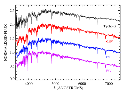
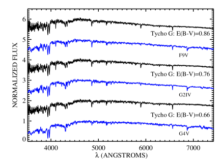
Figure 1: Left panel: Keck LRIS spectrum of Tycho G compared with three template spectra having spectral types G2 IV, F8 I, and F6 V taken from a library of low-resolution stellar spectra (Jacoby et al. 1984). The absorption feature near 6900 Å in the template spectra is the telluric B band. Another, weaker telluric feature is visible near 7200 Å. Right panel: LRIS spectrum of Tycho G dereddened with $E(B-V)=0.66$, 0.76, and 0.86 mag, compared with spectra from the low-resolution library of Jacoby et al. (1984). The best fits to the different dereddened spectra of Tycho G are also shown.

With the aim of determining the spectral classification of several targets in the Tycho SN 1572 field, on 12 December 2007 we obtained spectra with the Low Resolution Imaging Spectrometer (LRIS; Oke et al. 1995) on the Keck I telescope. We used the 400/3400 grism, the 400/8500 grating, and the D560 dichroic, covering the range 3180–9150 Å. The full width at half-maximum (FWHM) resolution was 6.4 Å in the red part ($\lambda\gtrsim 5500$ Å) and 6.3 Å in the blue, with respective dispersions of 1.86 Å pixel^-1 and 1.09 Å pixel^-1. Tycho E, F, G, and D were observed in single exposures of 700, 200, 400, and 450 s, respectively; see Ruiz-Lapuente et al. (2004) for star identifications. The SNR of the individual spectra is 21, 37, 31, and 25 at 4600 Å for Tycho E, F, G, and D, respectively. These spectra were reduced using standard techniques (e.g., Foley et al. 2003), including removal of telluric absorption lines.

The spectrum of Tycho G is shown in Figure 1; spectra and classifications of the other stars are available in Appendix A. In general, our results do not support the spectral classifications suggested by Ihara et al. (2007), which are based on low-resolution ($\lambda/\Delta\lambda\approx 400$), low-SNR spectra obtained with the instrument FOCAS at the Subaru Telescope over a short spectral range (3600–4200 Å). Moreover, their relative flux calibrations are questionable since they apply a correction to the slope of each spectrum that is fitted when comparing with a template. Thus, we consider their spectral classifications to be unreliable.

3 Stellar Parameters

3.1 Low-Resolution Spectra

The blue and red parts of the LRIS spectra were merged and then rebinned at a scale of 2 Å pixel^-1. We compared the spectra of the four targets with a library of low-resolution stellar spectra from Jacoby, Hunter, & Christian (1984). We chose this library because the spectra have a similar resolution ($\sim$4.5 Å), with a dispersion of 1.4 Å pixel^-1, and cover a similar spectral region (3510–7427 Å) as our LRIS observations.

The low-resolution comparison with template spectra depends on the color excess applied to the LRIS spectra. We dereddened the calibrated spectra according to the parameterization of Cardelli, Clayton, & Mathis (1989), including the update for the near-ultraviolet given by O’Donnell (1994). Moreover, there is uncertainty in the spectral classification of each template. Thus, the spectral classification of stars using low-resolution spectra must always be considered only as an initial guess. The best fit is found for a reddening $E(B-V)=0.76$ mag, with $\chi 2_{\nu}=3.68$ (see below for details). This value of reddening was used in the comparison shown in Figure 1. In the library of Jacoby et al. (1984), there are not many spectra with luminosity class IV (only F0, F3, G2, G5 IV), whereas luminosity class V is very well sampled with several templates for each spectral type. If only low-resolution spectra are used to derive the spectral and luminosity classes, the results may be erroneous, since they depend on reddening and on the flux calibration of the observed spectra.

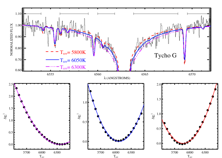
Figure 2: Upper panel: Synthetic H$\alpha$ profiles for three effective temperatures compared to the observed spectrum of Tycho G (SNR $\approx 30$) and normalized to the level of the observed spectrum of Tycho G at 6540 Å. We also display the fitting regions at the top. Lower panel: Results of $\chi 2_{\nu}$ analysis for three continuum positions separated by $\pm 1/{\rm SNR}=0.03$: 1.03 (left), 1.00 (middle), and 0.97 (right).

Nonetheless, as a first step, we compare the LRIS spectrum of Tycho G with the low-resolution spectra of three template stars having different spectral types (Fig. 1). To evaluate the goodness of fit, we employ a reduced $\chi 2$ statistic,

$$\chi 2_{\nu}=\frac{1}{N-M}\sum^{N}_{i=1}\left(\frac{f_{i}-F_{i}}{\sigma_{i}}\right)2,$$ (1)

where $N$ is the number of wavelength points, $M$ is the number of free parameters (here one), $f_{i}$ is the template flux, $F_{i}$ is the target flux (in this case, Tycho G), and $\sigma_{i}=1/{\rm SNR}$. The SNR was estimated as a constant average value in the continuum over the range 4610–4630 Å; this region was also used to normalize both target and template spectra. The spectral regions used to evaluate $\chi 2$ are 3850–6800 Å and 7000–7400 Å, avoiding strong telluric lines near 6900 Å present only in the template spectra.

The best fit is found for the G2 IV template with $\chi 2_{\nu}=3.68$, whereas the F8 I and F6 V templates provide $\chi 2_{\nu}=6.39$ and 9.66, respectively. Ihara et al. (2007) have claimed that the spectral type of Tycho G could be either F8 I, F8 V, or F6 V, rather than G2 IV as found by Ruiz-Lapuente et al. (2004). However, our analysis shows that those other spectral types provide worse fits than the G2 IV template.

Figure 3: Fe I and Fe II abundances computed using the best-fit atmospheric parameters of Tycho G (left panels) and two sets of stellar parameters: $T_{\rm eff}\;$$=5900$ K and $\log(g/{\rm cm~{}s}2)$ $=2$ dex (middle panels), $T_{\rm eff}\;$$=6200$ K and $\log(g/{\rm cm~{}s}2)$ $=4.35$ dex (right panels). Upper panels: Fe I abundance vs. excitation potential; middle panels: Fe I abundance vs. reduced equivalent widths; bottom panels: Fe II abundance vs. excitation potential. The dashed lines in the upper and middle panels represent the fits to the points, and in the bottom panels the mean abundance.

In the following sections we use more accurate classification methods, which are independent of reddening, to derive not only the spectral type of Tycho G but actually the effective temperature and surface gravity, using a high-resolution spectrum.

3.2 H$\alpha$ Profile

The wings of H$\alpha$ are a very good temperature indicator (e.g., Barklem et al. 2002). Adopting the theory of Ali & Griem (1965, 1966) for resonance broadening and Griem (1960) for Stark broadening, we computed H$\alpha$ profiles for several effective temperatures, using the code SYNTHE (Kurucz et al. 2005; Sbordone et al. 2005). For further details on the computations of hydrogen lines in SYNTHE, see Castelli & Kurucz (2001) and Cowley & Castelli (2002).

Figure 2 compares these synthetic H$\alpha$ profiles with the observed profile for several temperatures. To evaluate the goodness of fit, we employ the same method as in the previous section. However, in this case $M=1$ (the effective temperature $T_{\rm eff}$), $f_{i}$ is the synthetic normalized flux, $F_{i}$ is the observed normalized flux, and $\sigma_{i}=1/{\rm SNR}$. The SNR was estimated as a constant average value in continuum regions close to the observed H$\alpha$ profile. The fitting regions are indicated in Figure 2, which contains all of the spectral regions close the center of the H$\alpha$ profile where there are no stellar lines and where the normalized flux is greater than $\sim 0.7$. The best fit provided a temperature of $T_{\rm eff}\;$$=6050\pm 250$ K, with the error bars estimated from the best fits after displacing the observed continuum up and down by $1/{\rm SNR}=0.03$.

In the following section, we adopt the currently most reliable method for the determination of the stellar parameters.

3.3 Ionization Equilibrium of Iron

The best determination of the atmospheric parameters of Tycho G can be obtained from the ionization equilibrium of iron. We measured the equivalent widths of 32 Fe I and 10 Fe II isolated lines using an automatic line-fitting procedure which performs both line detection and Gaussian fits to unblended lines (François et al. 2003). The analysis was done using the 2002 version of the code MOOG (Sneden 1973) and a grid of local thermodynamic equilibrium (LTE) model atmospheres (Kurucz 1993). We adopted the atomic data from Santos, Israelian, & Mayor (2004), where the $\log gf$ values are adjusted until the solar atlas (Kurucz et al. 1984) is reproduced with a Kurucz model for the Sun having $T_{\rm eff}\;$$=5777$ K, $\log(g/{\rm cm~{}s}2)$ $=4.44$ dex, $\xi_{t}=1.00$ ${\rm km}\>{\rm s}^{-1}$, and $\log_{\odot}\epsilon(Fe)=7.47$ dex. This line list was designed to determine stellar parameters of planet-host stars with roughly the same atmospheric parameters and metallicity as Tycho G; it provides a compilation of 42 completely unblended Fe lines ideal for the determination of stellar atmospheric parameters. Note that none of the stellar lines used in this work for chemical analysis is affected by telluric lines.

The atmospheric parameters were determined by iterating until correlation coefficients between $\log\epsilon$(Fe I) and $\chi_{l}$, as well as between $\log\epsilon$(Fe I) and $\log(W_{\lambda}/\lambda)$, were zero, and the mean abundances from Fe I and Fe II lines were the same (see left panels of Fig. 3). The derived parameters were $T_{\mathrm{eff}}=5900\pm 100$ K, $\log(g/{\rm cm~{}s}2)$$=3.85\pm 0.30$ dex, $\xi_{t}=1.23\pm 0.23$ ${\rm km}\>{\rm s}^{-1}$, and $\mathrm{[Fe/H]}=-0.05\pm 0.09$. The uncertainties in the stellar parameters were estimated as described by Gonzalez & Vanture (1998). Thus, the uncertainties in $\xi_{t}$ and $T_{\rm eff}\;$take into account the standard deviation of the slope of the least-squares fits, $\log\epsilon$(Fe I) versus $\log(W_{\lambda}/\lambda)$ and $\log\epsilon$(Fe I) versus $\chi_{l}$. The uncertainty in $\log\;g\;$ considers the uncertainty on $T_{\rm eff}\;$in addition to the scatter of the Fe II abundances. Finally, the uncertainty in Fe abundance is estimated from a combination of the uncertainties in $\xi_{t}$ and $T_{\rm eff}\;$, in addition to the scatter of the Fe I abundances, all added in quadrature.

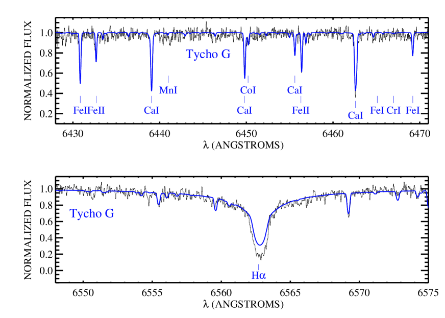
Figure 4: Best synthetic spectral fits (solid lines) to the Keck HIRES spectrum of Tycho G for two spectral regions. The core of the H$\alpha$ line suffers from NLTE effects that are not taken into account in our LTE synthetic spectrum.

In Figure 3, we also show two set of stellar parameters, $T_{\rm eff}\;$$=5900$ K and $\log(g/{\rm cm~{}s}2)$ $=2$ dex (middle panels), and $T_{\rm eff}\;$$=6200$ K and $\log(g/{\rm cm~{}s}2)$ $=4.35$ dex (right panels), corresponding to the spectral types F8 I and F6-7 V (Gray 1992). The lower-middle and upper-middle panels show inconsistent abundances between Fe I and Fe II, whereas the upper-right panel shows a negative slope for iron abundance versus excitation potential $\chi_{l}$ of the spectral lines Fe I. Therefore, these two sets of parameters cannot be the stellar parameters of Tycho G. According to the spectral classification provided by Gray (1992), the stellar parameters of Tycho G correspond to a spectral type of G0-1 IV.

Non-LTE (NLTE) corrections for stars with similar stellar parameters and metallicity have been estimated at $\lesssim 0.07$ dex for Fe I lines, while Fe II seems to be insensitive to NLTE effects (Thévenin & Idiart 1999). In addition, Santos et al. (2004) compared spectroscopic surface gravities with $\log g$ using Hipparcos parallaxes and found an average difference of $\sim+0.03$ dex, which might in fact reflect NLTE effects on Fe I lines. Our assumption of LTE seems to be accurate enough to determine the surface gravity of the star within the error bars. Note that ionization equilibrium also holds for Si and Cr (see § 4).

This determination of effective temperature is consistent within the error bars with that derived from the H$\alpha$ profile ($T_{\rm eff}\;$$=6050\pm 250$ K). However, echelle spectrographs are not ideally suited for measuring the shape of broad features such as the wings of Balmer lines (Allende Prieto et al. 2004), and the SNR of $\sim$30 is not high enough for the determination of effective temperature from the H$\alpha$ profile with great accuracy. For this reason, we will adopt the $T_{\rm eff}\;$$=5900\pm 100$ K value for the determination of the chemical abundances.

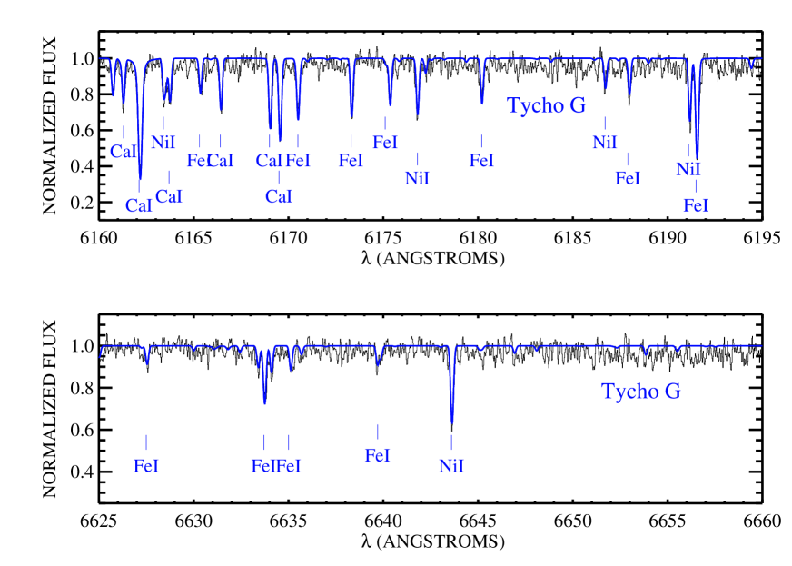
Figure 5: Same as Fig. 4, but for other spectral regions.

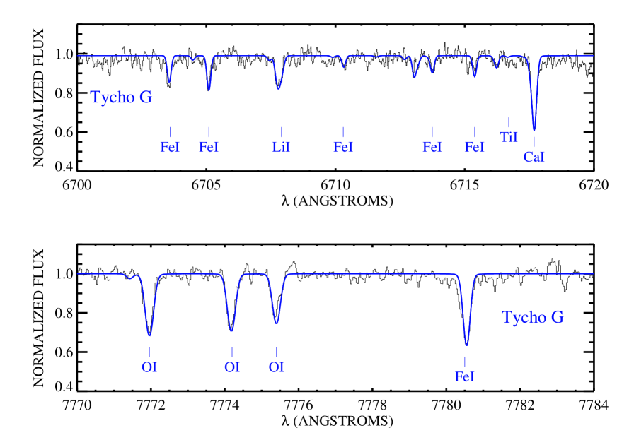
Figure 6: Same as Fig. 4, but for other spectral regions.

4 Chemical Abundances

Using the derived stellar parameters, we determine the element abundances from the absorption-line equivalent width (EW) measurements of the elements given in Table 4, except for lithium and sulfur for which we use a $\chi 2$ procedure to find the best fit to the observed features (e.g., González Hernández et al. 2004, 2005, 2006). The atomic data for O, C, S, and Zn are taken from Ecuvillon, Israelian, & Santos (2004, 2006), those of Na, Mg, Al, Si, Ca, Sc, Ti, V, Cr, Mn, Co, and Ni are from Gilli, Israelian, & Ecuvillon (2006), and those for Sr, Y, and Ba are from Reddy et al. (2003).

In Figures 4, 5, and 6 we display several spectral regions of the observed spectrum of Tycho G in comparison with synthetic spectra computed using the derived element abundances. Uncertainties in the abundances of all elements were then determined, adding in quadrature the errors due to the sensitivities of the resulting abundances to changes in assumed atmospheric parameters and the dispersion of the abundances from individual lines of each element.

In Table 1 we provide the average abundance of each element together with the errors. The errors in the element abundances show their sensitivity to the uncertainties in the effective temperature ($\Delta_{T_{\mathrm{eff}}}$), surface gravity ($\Delta_{\log g}$), microturbulence ($\Delta_{\xi}$), and the dispersion of the measurements from different spectral features ($\Delta_{\sigma}$). The errors $\Delta_{\sigma}$ were estimated as $\Delta_{\sigma}=\sigma/\sqrt{N}$, where $\sigma$ is the standard deviation of the $N$ measurements.

Table 1: Chemical Abundances of Tycho G

Species	$\log\epsilon(\mathrm{X})_{\odot}$	$[{\rm X}/{\rm H}]$	$[{\rm X}/{\rm Fe}]$	${\sigma}$	$\Delta_{\sigma}$	$\Delta_{T_{\rm eff}}$	$\Delta_{\log g}$	$\Delta_{\xi}$	$\Delta\mathrm{[X/H]}$	$\Delta\mathrm{[X/Fe]}$	$n$
C I	8.56	-0.15	-0.07	0.15	0.07	-0.06	0.09	0	0.13	0.19	5
O I	8.74	-0.02	0.03	0.02	0.01	-0.08	0.07	-0.02	0.11	0.18	3
Na I	6.33	0.04	0.09	0.18	0.10	0.05	-0.05	-0.02	0.12	0.12	3
Mg I	7.58	0.08	0.13	0.06	0.03	0.05	-0.04	-0.03	0.08	0.06	4
Al I	6.47	0.16	0.21	0.05	0.03	0.06	-0.01	-0.01	0.07	0.05	2
Si I	7.55	-0.03	0.02	0.09	0.02	0.04	-0.01	-0.02	0.05	0.05	12
Si II	7.55	-0.03	0.02	–	–	-0.08	0.11	-0.03	0.14	0.20	6371
S I	7.21	-0.02	0.03	0.07	0.05	-0.03	0.12	0	0.13	0.18	2
Ca I	6.36	-0.04	0.01	0.11	0.03	0.08	-0.04	-0.05	0.11	0.05	10
Sc II	3.10	-0.06	-0.01	0.09	0.03	0.01	0.12	-0.04	0.13	0.15	7
Ti I	4.99	-0.03	0.02	0.14	0.04	0.11	0	-0.02	0.12	0.06	10
V I	4.00	0.07	0.12	0.21	0.07	0.10	-0.01	-0.01	0.12	0.08	8
Cr I	5.67	-0.04	0.01	0.16	0.05	0.07	0	-0.01	0.09	0.06	9
Cr II	5.67	-0.03	0.02	–	–	-0.02	0.11	-0.04	0.12	0.16	5305
Mn I	5.39	0.02	0.07	0.15	0.05	0.09	-0.02	-0.05	0.12	0.06	8
Fe I	7.47	-0.05	0	0.12	0.02	0.08	-0.01	-0.04	0.09	–	32
Fe II	7.47	-0.05	0	0.10	0.03	0	0.13	-0.05	0.14	0.17	10
Co I	4.92	0.13	0.18	0.14	0.07	0.09	0	-0.02	0.12	0.08	4
Ni I	6.25	0.11	0.16	0.19	0.04	0.08	-0.01	-0.04	0.10	0.04	22
Zn I	4.60	-0.06	-0.01	0.09	0.05	0.03	0.02	-0.08	0.10	0.09	3
Sr I	2.64	0.07	0.12	–	–	0.09	-0.02	-0.06	0.11	0.03	4607
Y II	2.12	-0.14	-0.09	0.16	0.08	0.02	0.12	-0.06	0.16	0.17	4
Ba II	2.20	0.19	0.24	0.12	0.07	0.03	0.05	-0.17	0.19	0.17	3

Note. — Chemical abundances of Tycho G and uncertainties produced by $\Delta({T_{\rm eff}})=+100$ K, $\Delta({\log g})=+0.3$ dex, and $\Delta({\xi})=+0.23~{}$${\rm km}\>{\rm s}^{-1}$.

The abundances of several elements listed in Table 1 relative to iron are compared in Figures 7, 8, and 9 with the Galactic trends of these elements in the relevant range of metallicities. The abundances of some heavy elements relative to iron are above the solar values. The value found for [Ni/Fe], $0.16\pm 0.04$, is well above the average value if we consider the intrinsic dispersion ([Ni/Fe] $=-0.07\pm 0.04$, see Fig. 9) for the stars with similar metallicity of Tycho G ([Fe/H] $=-0.05\pm 0.09$). In Figure 5 we display several spectral ranges where some Ni I lines are well reproduced. Generally, Ni tracks Fe throughout the [Fe/H] range down to [Fe/H] $=-1$. The average value and scatter found by Reddy, Lambert, & Allende Prieto (2006) is [Ni/Fe] $=-0.05\pm 0.02$ for thin-disk stars and [Ni/Fe] $=-0.01\pm 0.04$ for thick-disk stars. Bensby et al. (2005) found [Ni/Fe] $=-0.06\pm 0.04$ for thin-disk stars and [Ni/Fe] $=-0.02\pm 0.02$ for thick-disk stars. This suggests pollution in Ni by Tycho SN 1572 ejecta. We find in general solar or slightly above solar abundances of heavy elements, while the $\alpha$ elements are consistent with the solar value or below.

Figure 7: Abundance ratios of Tycho G (wide cross) in comparison with the abundances of G and K metal-rich dwarf stars. Galactic trends were taken from Ecuvillon et al. (2004), Ecuvillon et al. (2006), and Gilli et al. (2006). The size of the cross indicates the $1\sigma$ uncertainty. For the abundance of oxygen in metal-rich dwarfs, we have only considered abundance measurements in NLTE for the triplet O I 7771–5 Å. The dashed-dotted lines indicate solar abundance values.

The binary companions of black holes or neutron stars show a different enhancement of metals with respect to the solar values. These stars exhibit significant enrichment in $\alpha$ elements. For instance, the black hole binary Nova Scorpii 1994 ([Fe/H] = –0.1) shows enhancements of [$\alpha$/Fe] = 4–8 in Mg, S, Si, and O (González Hernández et al. 2008a). The pollution seems to be related to the fallback of the ejected material of the supernova. In SNe Ia, one does not expect fallback of material onto the companion star since the compact object (the white dwarf in this case) is destroyed and the gravitational potential well is not sufficiently deep to retain the ejected material. Therefore, one expects to have a low contamination in intermediate-mass elements. The material captured by the companion should consist of heavy elements; they are less likely to escape the companion star since they move at lower velocities in the supernova ejecta. A discussion of this is given in § 8.1.

Another feature of interest in Tycho G is its high lithium abundance; the Li line at 6708 Å is pronounced. Modeling the Li abundance gives $A$(Li) = $2.50\pm 0.09$. The lithium abundance is provided here as $A$(Li) $=\log[N({\rm Li})/N({\rm H})]+12$ and takes into account NLTE effects. The NLTE abundance correction, $\Delta_{\mathrm{NLTE}}=\log\epsilon(\mathrm{X})_{\mathrm{NLTE}}-\log\epsilon(\mathrm{X})_{\mathrm{LTE}}$, for Li was derived from the theoretical LTE and NLTE curves of growth in Pavlenko & Magazzù (1996).

Figure 8: Same as Fig. 7, but for different elements.

The high Li abundance in Tycho G is intriguing since Li is easily destroyed in the convective envelopes of stars that have evolved away from the main sequence. Subgiants with $A$(Li) $>$ 2.2 are rare. Thorén, Edvardsson, & Gustafsson (2004) found that subgiants with detected Li divide into two groups: the stars with $T_{\rm eff}<5500$ K have $A$(Li) $\leq$ 1.5, and a warmer group of stars have higher abundances, although still much lower than their primordial abundances, with $A$(Li) $\leq$ 2.2. This seems to go in the direction of confirming post-main-sequence evolution toward lower amounts of Li as expected from stellar models.

Figure 9: Same as Fig. 7, but for different elements.

Tycho G shares a high Li content with a known sample of binary companions of neutron stars and black holes (Martín et al. 1994a; González Hernández et al. 2004, 2005). However, we know that cataclysmic variables, whose compact objects are white dwarfs, do not show such high Li abundances (Martín et al. 1995). We discuss this further in § 8.2.

Table 2: Distance of Tycho G

Parameter	$E(B-V)\tablenotemark{a}=0.76$	$E(B-V)\tablenotemark{a}=0.66$	$T_{\rm eff}\;$$\tablenotemark{b}=5800$ K	$\log\;g\;$$\tablenotemark{c}=4.15$	$\log\;g\;$$\tablenotemark{d}=3.55$	$M_{\star}\tablenotemark{e}=0.8~{}\hbox{\hbox{M}${}_{\odot}$}$
$R_{\star}(\hbox{\hbox{R}${}_{\odot}$})$	1.87	1.87	1.87	1.32	2.63	1.67
$L_{\star}$ (L⊙)	3.80	3.80	3.54f	1.90	7.57	3.04
$d_{m_{V}}\tablenotemark{f}$ (kpc)	$3.80\pm 0.07$	$4.39\pm 0.08$	$3.65\pm 0.07$	$2.69\pm 0.05$	$5.38\pm 0.10$	$3.40\pm 0.06$
$d_{m_{R}}$ (kpc)	$3.52\pm 0.05$	$3.98\pm 0.06$	$3.41\pm 0.05$	$2.49\pm 0.03$	$4.99\pm 0.07$	$3.15\pm 0.04$
$d_{m_{J}}$ (kpc)	$3.49\pm 0.11$	$3.65\pm 0.12$	$3.43\pm 0.11$	$2.47\pm 0.08$	$4.94\pm 0.16$	$3.12\pm 0.10$
$d_{m_{H}}$ (kpc)	$3.09\pm 0.15$	$3.22\pm 0.16$	$3.06\pm 0.15$	$2.20\pm 0.11$	$4.37\pm 0.22$	$2.77\pm 0.14$
$d_{m_{K}}$ (kpc)	$3.16\pm 0.18$	$3.25\pm 0.18$	$3.13\pm 0.18$	$2.24\pm 0.13$	$4.46\pm 0.25$	$2.82\pm 0.16$
$d_{\rm av}^{g}$ (kpc)	$3.50\pm 0.31$	$3.85\pm 0.52$	$3.40\pm 0.25$	$2.48\pm 0.21$	$4.95\pm 0.44$	$3.13\pm 0.27$

5 Distance

One can estimate the distance of Tycho G from different photometric colors and stellar parameters. We use the photometric magnitudes in five different filters: $m_{V}=18.71\pm 0.04$ and $m_{R}=17.83\pm 0.03$ mag from Ruiz-Lapuente et al. (2004), and $m_{J}=15.84\pm 0.07$, $m_{H}=15.16\pm 0.11$, and $m_{K}=15.03\pm 0.12$ mag from the 2MASS catalog. We derived the radius of the star from the surface gravity, $\log(g/{\rm cm~{}s}2)$ $=3.85\pm 0.3$ dex, and assuming a mass of 1 M_⊙. This radius, together with the spectroscopic estimate of the effective temperature, $T_{\rm eff}\;$$=5900\pm 100$ K, provides an intrinsic bolometric luminosity of $1.9<L_{\star}/L_{\odot}<7.6$.

In Table 2, we show distance determinations for the different filters, using the bolometric corrections for models without overshooting (Bessell, Castelli, & Plez 1998), for our preferred value of the color excess, $E(B-V)=0.76$ mag, and other different sets of the relevant parameters. We compute the magnitude corrected for extinction in each filter as $m_{V,0}=m_{V}-A_{V}$, where $A_{V}=3.12\,E(B-V)$ is the extinction in the Johnson $V$ filter. We adopt the following values for other filters (Schaifers et al. 1982): $A_{R}/A_{V}=0.84$, $A_{J}/A_{V}=0.32$, $A_{H}/A_{V}=0.27$, and $A_{K}/A_{V}=0.21$.

Table 2 clearly shows the uncertainty in the distance due to the uncertainty in the stellar parameters of Tycho G. Note that the relatively small formal error in the distance estimate for each filter is calculated by assuming that the magnitudes equal $m_{i}+\Delta m_{i}$.

In Table 2, we also show for each set of parameters the average distance determinations weighted by the uncertainty of each individual distance determination. These values cover a distance range 2.48–4.95 kpc with errors of 0.21–0.52 kpc. We have also considered the possibility that Tycho G lost part of its envelope, $\Delta M=-0.2$ M_⊙, due to the impact of the supernova shock wave (Marietta, Burrows, & Fryxell 2000; Pakmor et al. 2008). However, a lower mass does not produce a significant change in the derived average distance. In all cases, we have assumed that the companion star is able to almost completely recover thermal equilibrium between $\sim 102$ and $\sim 103$ yr after the white dwarf explosion (Podsiadlowski 2003). The distance to the SN 1572 remnant inferred from the expansion of the radio shell and by other methods is $2.83\pm 0.79$ kpc (Ruiz-Lapuente 2004). Such a distance is in good agreement with the derived distances of Tycho G.

6 Projected Rotational Velocity of Tycho G

Tycho G is not a fast rotator, unlike the companion stars of Type II SNe. The projected rotational velocity is constrained by the instrumental resolution to $v_{\rm rot}\,{\rm sin}\,i\leq 6.6$ km s^-1.

However, the companion stars of SNe II and other core-collapse SNe have different rotational histories from those proposed for SN Ia progenitors; they would be massive stars, and maybe fast rotators (Meynet & Maeder 2005, and references therein). Moreover, the orbital elements just before the explosion are also different; in particular, the separations are larger. Given the orbital history up to the explosion, it is reasonable to find fast rotators around black holes and neutron stars (González Hernández et al. 2004, 2005, 2008b). The companion stars of these compact objects do not transfer mass to the star that becomes a core-collapse supernova. If the explosion does not unbind the system, the companion can be seen as a star orbiting a black hole or neutron star and showing significant rotational velocity. But, for SNe Ia, we should not expect such high velocities since the companion of the white dwarf would have transferred mass and angular momentum to the white dwarf. And, after the impact, the loss of the envelope would have further helped decrease the angular momentum and to brake rotation.

Let us consider, for instance, a WD mass $M_{WD}=1.4$ M_⊙ and a companion of mass $M=1$ M_⊙ (a system similar to U Scorpii; see, e.g., Thoroughgood et al. 2001). In such a system, an orbital velocity of 90 ${\rm km}\>{\rm s}^{-1}\;$(this value could roughly correspond to the peculiar velocity of Tycho G estimated by Ruiz-Lapuente et al. 2004, still consistent with the values from the present work) corresponds to an orbital separation $a=19.28$ R_⊙ and an orbital period $P_{\rm orb}=6.32\ {\rm d}$. The effective Roche lobe radius of the companion can be calculated from the Eggleton (1983) approximation (accurate up to a few percent for all mass ratios):

$$R_{L}=a\left[{0.49\over 0.6+q^{-2/3}\ {\rm ln}(1+q^{1/3})}\right].$$ (2)

It would then be $R_{L}=6.75$ R_⊙.

Assuming that tidal interaction had been effective enough to keep the rotational period of the companion locked with the orbital period in spite of the angular momentum loss due to mass transfer, and that no further changes have intervened, the rotation period of the companion should now be $P_{\rm rot}=P_{\rm orb}=6.32\ {\rm d}$. Therefore, the rotational velocity is $v_{\rm rot}=2\pi R/P_{\rm rot}$. However, the present radius of the Tycho G is within the range $R\approx 1$–2 R_⊙, as can be seen from its position in the Hertzsprung-Russell diagram. This then gives $v_{\rm rot}\approx 8$–16 ${\rm km}\>{\rm s}^{-1}$. Here we have assumed that the impact of the SN ejecta has removed the outer, more distended and less gravitationally bound layers (Marietta et al. 2000; Pakmor et al. 2008), and that the star is able to completely or partially recover thermal equilibrium $\sim 500$ yr after the explosion (Podsiadlowski 2003). In this case, when the energy deposited on the star due to the impact of the shock wave of the supernova is $\lesssim 5\times 10^{46}$ erg, the luminosity of the star in the time interval $\sim 102$–$103$ yr after the explosion could be roughly $\sim 2$–5 L_⊙. Hence, the radius of the star would be in the range $\sim 1.5$–2 R_⊙.

Thus, an observed value of $v_{\rm rot}\,{\rm sin}\ i\leq 6.6$ ${\rm km}\>{\rm s}^{-1}\;$is not an unexpected result in this case (for a typical angle $i\approx 45^{o}$ or lower). In fact, the preceding analysis does not even take into account angular momentum losses due to mass stripping, nor the slowing down of rotation (with conservation of angular momentum) that would result from puffing up of the fraction of the envelope remaining bound.

Any suggestion that the rotational velocity of the former companion of a SN Ia should now be very high is based on the possibly incorrect assumption that its current radius should remain, after the SN Ia explosion, at the large value it had at the time of Roche-lobe filling (equal to 6 R_⊙ in our example). Thus, expected rotational velocities of companions of supernovae, as well as potential pollution by the supernova ejecta, are different in SNe Ia and SNe II/Ib/Ic.

7 Space Velocity and Position of Tycho G

In our previous study (Ruiz-Lapuente et al. 2004), we measured the proper motion of Tycho G to be $\mu_{b}=-6.11\pm 1.34$ mas yr^-1 and $\mu_{l}=-2.6\pm 1.34$ mas yr^-1. The proper motion in Galactic latitude implies that the star is an outlier in proper motion, with a derived tangential velocity of $94\pm 27$ ${\rm km}\>{\rm s}^{-1}$. A new, more accurate and precise proper motion is currently being derived from HST images obtained in Cycle 16.

The spectral data presented by Ruiz-Lapuente et al. (2004) allowed an estimate of the heliocentric radial velocity of Tycho G with an uncertainty of 10–18 ${\rm km}\>{\rm s}^{-1}$. The new Keck HIRES data provide a much smaller uncertainty. For this new measurement we selected six strong, unblended lines in the spectral range 6000–8000 Å and measured the radial velocity of each individual line. The average radial velocities from those lines are found to be $-87.36\pm 0.60$ ${\rm km}\>{\rm s}^{-1}\;$and $-87.53\pm 0.48$ ${\rm km}\>{\rm s}^{-1}\;$during the first and second nights, respectively, where the errors indicate the dispersion of the measurements. The average of the two epochs is $v_{r}=-87.4\pm 0.5$ ${\rm km}\>{\rm s}^{-1}$. This value implies that $v_{r}\approx-80$ ${\rm km}\>{\rm s}^{-1}\;$in the local standard of rest (LSR). In our previous measurement, we had quoted $v_{r}=-99\pm 6$ ${\rm km}\>{\rm s}^{-1}\;$ (statistical error). The measurement was made using H${\alpha}$ and H${\beta}$ lines, which are worse indicators of the velocity of the star.

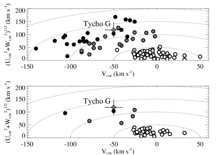
Figure 10: Upper panel: Toomre diagram of the thick-disk stars (black filled circles), thin-disk stars (open circles), and transition stars (grey filled circles) from Bensby et al. (2003, 2005). The star Tycho G is displayed as a rhombus. Lower panel: the same as upper panel, but for stars with metallicity greater than or equal to the metallicity of Tycho G.

Stars in the direction of the Tycho SN remnant at distances of 2–4 kpc move at an average radial velocity $v_{r}\approx-20$ to $-40$ ${\rm km}\>{\rm s}^{-1}\;$(in the LSR), in agreement with Galactic rotation models (Brand & Blitz 1993; Dehnen & Binney 1998). Tycho G is well above the average of stars in its vicinity. Both the radial velocity and the proper motion show a comparably high velocity. One could argue that Tycho G might be at a larger distance (although this seems unlikely from its photometric magnitudes; see § 5), but the observed proper motion would make the tangential velocity unreasonably high if the star were $>6$ kpc away ($v_{t}\approx 187$ ${\rm km}\>{\rm s}^{-1}\;$at $d=6$ kpc). On the other hand, a distance of 4–5 kpc (although $v_{t}\approx 140$ ${\rm km}\>{\rm s}^{-1}\;$at $d=4.5$ kpc) might not be ruled out by these arguments, albeit somewhat inconsistent with the estimated distance of the Tycho SN 1572 remnant ($2.83\pm 0.79$ kpc; Ruiz-Lapuente 2004).

However, Fuhrmann (2005) has argued, based on the Galactic space velocity components of Tycho G relative to the LSR ($U_{\rm LSR},V_{\rm LSR},W_{\rm LSR}$), that this star could be just a thick-disk star passing close to the SN remnant. Assuming that the Sun moves with components $(U_{\odot,{\rm LSR}},V_{\odot,{\rm LSR}},W_{\odot,{\rm LSR}})=(10.,5.2,7.2)$ ${\rm km}\>{\rm s}^{-1}\;$(Dehnen & Binney 1998) relative to the LSR, for distance of 3 kpc, we estimate the space Galactic velocity components of Tycho G to be $(U_{\rm LSR},V_{\rm LSR},W_{\rm LSR})=(85\pm 17,-50\pm 10,-82\pm 24)$ ${\rm km}\>{\rm s}^{-1}$. In Figure 10 we display Galactic velocity of Tycho G in comparison with the Galactic velocities of thick-disk and thin-disk stars. Although the Galactic velocity of Tycho G is comparable to that of thick-disk stars, its metallicity is more common in thin-disk stars. In the lower panel of Figure 10, we display only those stars with metallicity equal to or greater than the metallicity of Tycho G. The number of thick-disk stars is reduced considerably, but there are still a few thick-disk stars with the same metallicity and Galactic velocity as Tycho G. On the other hand, the high Ni abundance of Tycho G would be very unusual for a thick-disk star. We therefore conclude that while a thick-disk origin may be consistent with the data, this possibility is not favored because it provides no explanation for the anomalous Ni abundance.

Although the position of Tycho G in the sky does not coincide with the proposed geometrical center of the X-ray and radio remnants of SN 1572, the offset of the position is within the uncertainties due to the asymmetry resulting from interaction of the expanding remnant with the circumstellar medium. Indeed, there is $0.56^{\prime}$ displacement along the E–W axis between the radio emission and the high-energy continuum observed by XMM-Newton, in the position of the western rim (Decourchelle et al. 2001). Such asymmetry amounts to a 14% offset along the E–W axis. It appears to be due to the ejecta having encountered a dense H cloud at the eastern edge, giving rise to brighter emission and lower expansion velocity of the ejecta there, while interacting with a lower-density medium in the western rim. It was precisely owing to those considerations that we studied all of the 23 stars with $m_{V}\leq 22$ mag within a circle of radius $0.65^{\prime}$ around the geometrical center of the X-ray emission as given by the Chandra observations (Hughes 2000). All of the stars within that circle were considered on an equal footing as possible companions until all were discarded with the exception of Tycho G, due to the unique characteristics of this star. In the next two sections, we discuss its chemical peculiarities.

Table 3: Supernova Ia models in Tycho G

			${\rm[X/H]\>EXPECTED}\tablenotemark{c}$
ELEMENT	${\rm[X/H]\>\rm OBSERVED}\tablenotemark{a}$	${\rm[X/H]}_{0}\tablenotemark{b}$	W7	W70	WDD1	WDD2	WDD3	CDD1	CDD2
O	$-0.02\pm 0.11$	$-$0.15	$-$0.14	$-$0.14	$-$0.14	$-$0.15	$-$0.15	$-$0.14	$-$0.15
Na	$0.04\pm 0.12$	$-$0.26	$-$0.26	$-$0.26	$-$0.26	$-$0.26	$-$0.26	$-$0.26	$-$0.26
Mg	$0.08\pm 0.08$	$-$0.10	0.04	0.13	0.03	$-$0.02	$-$0.05	0.03	$-$0.02
Al	$0.16\pm 0.07$	$-$0.06	$-$0.05	$-$0.06	$-$0.06	$-$0.06	$-$0.06	$-$0.06	$-$0.06
Si	$-0.03\pm 0.05$	$-$0.22	$-$0.07	$-$0.08	0.02	$-$0.03	$-$0.06	0.02	$-$0.03
S	$-0.02\pm 0.13$	$-$0.26	$-$0.10	$-$0.10	$-$0.00	$-$0.05	$-$0.09	0.00	$-$0.06
Ca	$-0.04\pm 0.11$	$-$0.31	$-$0.15	$-$0.08	0.03	$-$0.03	$-$0.08	0.03	$-$0.03
Ti	$-0.03\pm 0.12$	$-$0.06	0.00	0.02	0.12	0.10	0.09	0.08	0.07
Cr	$-0.04\pm 0.09$	$-$0.27	0.03	0.05	0.27	0.21	0.16	0.24	0.20
Mn	$0.02\pm 0.12$	$-$0.27	0.12	0.05	0.11	0.06	0.03	0.09	0.05
Fe	$-0.05\pm 0.09$	$-$0.21	0.11	0.12	0.09	0.13	0.15	0.08	0.14
Co	$0.13\pm 0.12$	$-$0.14	0.03	0.02	$-$0.07	$-$0.03	$-$0.01	$-$0.09	$-$0.03
Ni	$0.11\pm 0.10$	$-$0.27	0.40	0.32	0.06	0.16	0.23	0.04	0.18

8 Discussion

8.1 Has Tycho G been Polluted by the SN Ia?

The measured ratio [Ni/Fe] $=0.16\pm 0.04$ in Tycho G is 4–5$\sigma$ above the average value of this ratio in the Galaxy ([Ni/Fe] $\approx-0.05$). It indicates an overabundance of Ni with respect to the Galactic trend. Ni may have been trapped by the star as slowly moving material from deep layers of the SN ejecta orbited around it. While the rapidly moving ejecta consisting mainly of intermediate-mass elements would have escaped away from the site of the explosion, the very slowly moving tail made of heavy elements like Ni could have been captured by the companion.

To be consistent with the evolutionary path suggested above (and also by Ruiz-Lapuente et al. 2004), we use $a=19.28$ R_⊙ for the separation between the white dwarf and its companion, and $R_{*}=R_{L}=6.75$ R_⊙ for the radius of the companion (just before the SN explosion).

The mass that could be trapped by the companion is given by the subtended angle,

$$m_{\rm t}=\Delta M\ (\pi R_{2}^{2}/4\pi\ a^{2})\ f,$$ (3)

where $\Delta M$ is the ejected mass and $f$ is the fraction of retained material.

We try to model the contamination of the companion star by the nucleosynthetic products of different SN Ia models from Iwamoto et al. (1999). In Table 3 we show the expected abundances of Tycho G after having captured a significant amount of the SN ejecta. In these model computations, we adopt the yields from SN Ia models with different kinetic explosion energies in the range (1.30–$1.44)\,\times\,10^{51}$ ergs, different central densities (in units of $109$ g cm^-3) of $\rho_{9}=1.37$ (C) and 2.12 (W), and different deflagration velocities with fast deflagration in the models W7 and W70 (Nomoto, Thielemann, & Yokoi 1984) and slow deflagration in the others. We assumed as initial abundances the average abundances of disk stars with a metallicity of ${\rm[Fe/H]}=-0.20\pm 0.09$, and a capture efficiency factor $f=0.03$. The matter that is captured by the companion has a much larger mean molecular weight than the composition of its atmosphere and then is completely mixed with the whole star due to thermohaline mixing, in a short timescale (Podsiadlowski et al. 2002).

Badenes et al. (2006) found, by comparing a grid of X-ray synthetic spectra based on hydrodynamical models, that the fundamental properties of X-ray emission in Tycho SN 1572 are well reproduced with one-dimensional delayed detonation models having a kinetic energy of $\sim 1.2\,\times\,10^{51}$ ergs. In Table 3, the models called WDD1,2,3 and CDD1,2 include transitions from slow deflagration to detonation, which are equivalent to delayed detonation models.

In Figure 11, we display the observed abundances of Tycho G in comparison with the expected abundances from several SN Ia models. Except for Na and Al, we find reasonable agreement between the observed abundances of Tycho G and the expected abundances after contamination from the nucleosynthetic products of the SN Ia. Surprinsingly, González Hernández et al. (2008a) measured the chemical abundances of the secondary star of the black hole binary Nova Scorpii 1994 and found several $\alpha$ elements significantly enhanced in the companion star while Al and Na were not enhanced. The enhanced $\alpha$ elements in that star were explained by comparing the observed abundances with supernova/hypernova explosion models. However, these models also predict that Al and Na should be enhanced at a comparable level as oxygen, and they did not find an explanation for this discrepancy. Therefore, the model of contamination of Tycho G by using SN Ia models could provide an explanation for the relatively high observed [Ni/Fe] with respect to the Galactic trend of this element.

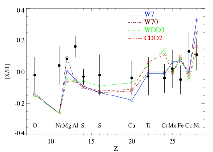
Figure 11: Expected abundances in Tycho G after contamination from the nucleosynthetic products in SN Ia models (Iwamoto et al. 1999), in comparison with the observed abundances.

One could find stable isotopes of Co as well among the slowly moving material in a SN Ia. The ratio [Co/Fe] $=0.18\pm 0.08$ in Tycho G is consistent with contamination from the SN ejecta. The study by Reddy et al. (2006) finds that [Co/Fe] shows flat behavior with [Fe/H] for thin-disk stars ([Co/Fe] $=-0.05\pm 0.02$). For thick-disk stars, a weak trend of decreasing [Co/Fe] with increasing [Fe/H] is apparent, falling to [Co/Fe] $=0.00\pm 0.04$ at the metallicity of Tycho G. The effect of a larger [Co/Fe] is $>1\sigma$, a lower significance level compared to the ratio [Ni/Fe] (see also Fig. 6). The ratios of the $\alpha$ elements (O, Si, Ca, and Ti) to iron do not show enhancements over Galactic values.

Figure 12: Li abundance of Tycho G in comparison with that of subgiant stars from Randich et al. (1999) having similar stellar parameters, metallicity, and rotational velocity.

A study of the SN 1572 remnant in X-rays (Hamilton et al. 1985) suggests that it contains $\sim$0.66 M_⊙, including 0.20 M${}_{\odot}\;$of Fe and 0.02 M${}_{\odot}\;$of Ni in an inner layer as well as $\sim$0.44 M${}_{\odot}\;$of Fe plus Ni unshocked by the reverse shock and consequently moving in free expansion. The energy of this supernova is estimated from the ejecta to be $E\approx$ (4–5) $\times 10^{50}$ ergs (Hughes 2000).

8.2 Li Abundance

As shown in Figure 6, the Li line at 6708 Å is pronounced in Tycho G. The abundance of this element, $A$(Li) = $2.50\pm 0.09$, raises the question of how much Li could have survived in this star that has already evolved off the main sequence. Similar abundances have been found in some turn-off stars (with $6300<T_{\rm eff}<6800$ K) in the sample of do Nascimento et al. (2000, 2003), and in a few subgiant stars with stellar parameters similar to those of Tycho G. In the sample of Randich et al. (1999), there are also a few subgiants with similar stellar parameters and Li abundance as Tycho G; see Figure 12. Although the Li abundance of Tycho G is somewhat high for its relatively low effective temperature and surface gravity, the upper-right panel of Figure 12 shows two stars (with $T_{\rm eff}\;$$\approx 5500$ K and 6000 K, and $\log(g/{\rm cm~{}s}2)$ $\approx 3.3$ dex) that are even more anomalous than Tycho G.

Canto Martins et al. (2006) found a Li-rich subgiant star (S1242) in the open cluster M67, with $T_{\rm eff}\;$$=5800$ K, $\log(g/{\rm cm~{}s}2)$ $=3.9$ dex, [Fe/H] $=-0.05$, and $A$(Li) = 2.7, all similar to the properties of Tycho G. This star is in a wide eccentric binary system, and these authors proposed that the Li has been preserved due to tidal effects. There exist other subgiant stars of similar type showing high Li abundances and belonging to binary systems. Again, this could be linked to being in a close binary system where tidal interaction might inhibit Li destruction.

An alternative is that Li was created as a result of energetic processes. Martín et al. (1992, 1994a,b) suggest that in soft X-ray transients (SXTs) one is observing freshly synthesized Li, and that the Li could come from $\alpha\alpha$ and/or other spallation reactions during the outbursts of these binary systems that contain black holes or neutron stars. Spallation reactions are produced by protons and $\alpha$ particles with energies above a few MeV when hitting C, N, and O nuclei, and also by $\alpha+\alpha$ collisions at similar energies.

In addition, in the case where the compact object is a white dwarf, Martín et al. (1995) have shown that their companion stars do not show high Li abundances. They claimed that this is consistent with the Li production scenario in SXTs, because the weaker gravitational potential well of the white dwarfs does not allow particles to be accelerated to the required high energies (Martín, Spruit, & van Paradijs 1994b). However, other authors have shown that Li production is possible during nova explosions (Starrfield et al. 1978; Boffin, Paulus, & Arnould 1993).

The energy arguments could also work for the enhancement of Li in the companion of a carbon-oxygen white dwarf. The accretion lasts for a sufficiently long time to build enough Li nuclei in the convective envelope of the secondary star. At the onset of the explosion, the supernova is able to unbind part of the material from the convective envelope. If part of the convective envelope were to survive, it would display a high Li abundance. However, this scenario of Li production during outbursts in SXTs also predicts Li isotopic ratios in the range $0.1<N(^{6}$Li)/$N(^{7}$Li$)<10$; see Casares et al. (2007), and references therein. These authors conclude that the preservation scenario by tidal effects is the most likely mechanism to explain the high Li abundances of SXTs.

There are two other alternatives for enrichment of Li in the companions of SNe Ia. The first is that the high-energy particles accelerated by the shock wave in the outermost layers of the exploding white dwarf induce spallation reactions in the surface of the companion. A fraction of the irradiated material could mix with the layers now making the surface of the companion, and Li enrichment would show. The second alternative is that the surface of the companion, after the explosion, can be bombarded by high-energy particles accelerated in the SN remnant, producing spallation reactions. Steady bombardment by those high-energy particles has the restriction that while it enriches Li, the energy deposited would increase the star’s luminosity. However, if Li enrichment is limited to a thin layer extending not much below the photosphere, the increase in luminosity would be negligible.

9 Overall Discussion of Tycho G

Ruiz-Lapuente et al. (2004) suggested Tycho G as the mass-donating companion of SN 1572 and gave stellar parameters that classified it as a G0–G2 IV star. In the present study, higher-resolution spectra have enabled us to pin down the stellar parameters: $T_{\rm eff}=5900\pm 100$ K, $\log(g/{\rm cm~{}s}2)$ $=3.85\pm 0.30$ dex, and [Fe/H] $=-0.05\pm 0.09$. Thus, we have been able to confirm that Tycho G has a metallicity close to solar and its luminosity class is that of a subgiant near the main sequence. Recently, Badenes et al. (2008) have estimated the global metallicity of the Tycho SN Ia remnant at $\log(Z_{\rm SN}/Z_{\odot})=0.45^{+0.31}_{-0.60}$ when adopting the solar abundances of Grevesse & Sauval (1998). We can estimate the global metallicity of the star by adding all the values of [X/H] provided in Table 1. The metallicity of Tycho G would be $\log(Z_{\rm TychoG}/Z_{\odot})\approx 0.23$, which is consistent with the value given by Badenes et al. (2008) within their large error bars.

Moreover, in support of the hypothesis that Tycho G is physically within the remnant of SN 1572 and is possibly the surviving companion of the supernova, we have found a high value of [Ni/Fe], $0.16\pm 0.04$, about 3$\sigma$ above the average value in Galactic disk stars ([Ni/Fe] $\approx-0.05\pm 0.03$). In addition, we report an anomalously high Li abundance for a subgiant, $A$(Li) $=2.50\pm 0.09$, although similar to a few other known subgiant stars having similar stellar parameters and metallicity.

The star is moving at high speed both in radial velocity and proper motion. If we consider the possibility that Tycho G is actually beyond the supernova remnant, at 6 kpc or more, where $v_{r,\rm LSR}=-80$ ${\rm km}\>{\rm s}^{-1}\;$would follow the low-latitude rotation pattern of the Galaxy, we run into two other physical incompatibilities: (a) at 6 kpc in the direction of SN 1572, the region has metallicities [Fe/H] $<-0.3$, much lower than observed for Tycho G; and (b) the tangential velocity implied by the observed proper motion and distance would be unreasonably high ($v_{t}\approx 187$ ${\rm km}\>{\rm s}^{-1}\;$at $d=6$ kpc). On the other hand, according to its space Galactic velocity components, Tycho G could be just a thick-disk star passing near the SN Ia remnant, but its high Ni abundance argues against this possibility.

We find that Tycho G has features in common with the companions of black holes and/or neutron stars that presumably originated in Type II SNe. These companions, which remain bound to the black hole or neutron star created by the explosion, are main-sequence stars and subgiants with a high Li abundance. The companions of core-collapse SNe are polluted with $\alpha$ elements, but Tycho G has an overabundance of Ni (and Co at lower significance level) with respect to Fe. The overabundance is well above the scatter for this ratio in Galactic disk stars, suggesting that Tycho G could have captured the low-velocity tail of the SN 1572 ejecta. We use SN Ia yields to model the possible contamination of the star from the SN ejecta and we find reasonable agreement with the observed abundances of Tycho G.

Thus, although the current evidence is not fully compelling, it remains consistent with Tycho G being the surviving companion star of the white dwarf that exploded to form SN 1572, as originally proposed by Ruiz-Lapuente et al. (2004).

Appendices

Appendix A Low-Resolution Spectra

We attempted to determine the spectral type of several stars in the Tycho SN 1572 field. In Figure 13 we display the best fits to the LRIS spectra of Tycho D, E, F, and G (see Ruiz-Lapuente et al. 2004 for identifications). The spectra of Tycho G and F were dereddened with $E(B-V)=0.76$ mag, whereas the spectrum of Tycho D was dereddened with $E(B-V)=0.66$ mag since this color excess provides a better fit to the LRIS spectrum. Based on the closer position of Tycho D and E to the center of the Tycho SN 1572 field, we also applied a color excess of $E(B-V)=0.66$ mag to Tycho E. However, we know from high-resolution spectra that Tycho E is in fact a double-lined spectroscopic binary, so this comparison using a low-resolution composite spectrum is meaningless. The spectral classifications of most stars differ from those published by Ihara et al. (2007), but are consistent with the results of Ruiz-Lapuente et al. (2004).

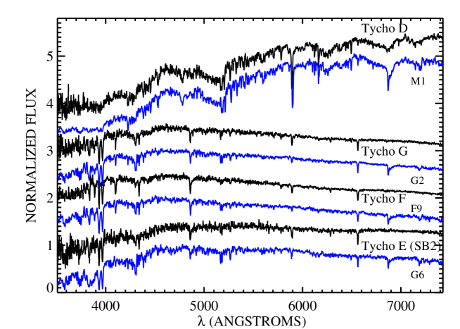
Figure 13: LRIS spectra of four targets of the Tycho SN 1572 field compared with template low-resolution spectra from the Jacoby et al. (1984) library. Note that telluric lines (B band near 6900 Å; weak lines around 7200 Å) were not removed from the templates. The spectra of Tycho G and F were dereddened with $E(B-V)=0.76$ mag, whereas $E(B-V)=0.66$ mag was used for the spectra of Tycho D and E. The best fit to each spectrum is also shown. Note that when Tycho E is observed at high resolution it seems to be a double-lined spectroscopic binary, and therefore the fit shown is not reliable.

Appendix B Line List with Equivalent Widths for Tycho G

Here we provide the complete list of line EWs measured from the high-resolution Keck spectra of Tycho G.

Table 4: Equivalent Widths of Lines in Tycho G

Species	$\lambda$	$\chi$	$\log(gf)$	EWλ	Species	$\lambda$	$\chi$	$\log(gf)$	EWλ
	(Å)	(eV)		(mÅ)		(Å)	(eV)		(mÅ)
Li I	6707.81	0.00	0.175	$38.7\pm 3.9$	Mn I	4502.220	2.920	-0.490	$60.3\pm 12.3$
					Mn I	5394.670	0.000	-3.500	$51.9\pm 4.7$
C I	5052.160	7.680	-1.420	$38.7\pm 7.0$	Mn I	5399.470	3.850	-0.097	$32.0\pm 4.7$
C I	6587.620	8.540	-1.000	$16.5\pm 3.8$	Mn I	5420.360	2.140	-1.460	$38.5\pm 4.6$
C I	7113.170	8.650	-0.770	$23.6\pm 3.3$	Mn I	5432.540	0.000	-3.620	$36.0\pm 4.5$
C I	7115.170	8.640	-0.930	$32.2\pm 3.3$	Mn I	6021.800	3.070	0.030	$91.0\pm 4.4$
C I	7116.960	8.650	-0.910	$25.3\pm 3.3$
					Fe I	5044.220	2.850	-2.040	$75.9\pm 7.0$
O I	7771.960	9.110	2.831	$94.7\pm 2.8$	Fe I	5247.060	0.090	-4.930	$58.0\pm 5.5$
O I	7774.180	9.110	2.061	$82.3\pm 2.8$	Fe I	5322.050	2.280	-2.900	$47.6\pm 5.1$
O I	7775.400	9.110	1.256	$68.0\pm 2.8$	Fe I	5806.730	4.610	-0.890	$50.3\pm 4.4$
					Fe I	5852.220	4.550	-1.190	$42.9\pm 4.4$
Na I	5688.220	2.104	-0.625	$117.4\pm 4.3$	Fe I	5855.080	4.610	-1.530	$12.4\pm 4.4$
Na I	6154.230	2.102	-1.607	$34.7\pm 3.8$	Fe I	5856.090	4.290	-1.560	$23.5\pm 4.4$
Na I	6160.750	2.104	-1.316	$40.1\pm 3.8$	Fe I	6027.060	4.080	-1.180	$56.4\pm 4.4$
					Fe I	6056.010	4.730	-0.500	$52.7\pm 4.3$
Mg I	4730.040	4.346	-2.390	$52.3\pm 9.4$	Fe I	6079.010	4.650	-1.010	$30.6\pm 4.2$
Mg I	5711.090	4.346	-1.706	$109.1\pm 4.3$	Fe I	6151.620	2.180	-3.300	$46.0\pm 3.8$
Mg I	6318.720	5.108	-1.996	$43.4\pm 3.6$	Fe I	6157.730	4.070	-1.240	$52.7\pm 3.8$
Mg I	6319.240	5.108	-2.179	$29.3\pm 3.6$	Fe I	6165.360	4.140	-1.500	$45.8\pm 3.8$
					Fe I	6180.210	2.730	-2.640	$46.1\pm 3.7$
Al I	6696.030	3.143	-1.570	$37.8\pm 4.0$	Fe I	6188.000	3.940	-1.630	$43.5\pm 3.7$
Al I	6698.670	3.143	-1.879	$26.1\pm 4.0$	Fe I	6200.320	2.610	-2.400	$73.0\pm 3.6$
					Fe I	6226.740	3.880	-2.070	$33.4\pm 3.6$
Si I	5665.560	4.920	-1.980	$47.0\pm 4.3$	Fe I	6229.240	2.840	-2.890	$27.1\pm 3.6$
Si I	5690.430	4.930	-1.790	$52.3\pm 4.3$	Fe I	6240.650	2.220	-3.290	$42.3\pm 3.6$
Si I	5701.100	4.930	-2.020	$32.2\pm 4.3$	Fe I	6265.140	2.180	-2.560	$71.6\pm 3.6$
Si I	5772.140	5.080	-1.620	$53.0\pm 4.4$	Fe I	6270.230	2.860	-2.580	$41.4\pm 3.6$
Si I	5793.090	4.930	-1.910	$44.9\pm 4.4$	Fe I	6392.540	2.280	-3.930	$11.8\pm 3.7$
Si I	5948.550	5.080	-1.110	$82.6\pm 4.5$	Fe I	6498.940	0.960	-4.630	$37.1\pm 3.7$
Si I	6125.020	5.610	-1.520	$38.9\pm 3.9$	Fe I	6608.030	2.280	-3.960	$17.9\pm 3.9$
Si I	6142.490	5.620	-1.480	$36.9\pm 3.9$	Fe I	6627.550	4.550	-1.480	$24.7\pm 3.9$
Si I	6145.020	5.610	-1.400	$35.2\pm 3.9$	Fe I	6703.570	2.760	-3.020	$29.6\pm 4.0$
Si I	6155.150	5.620	-0.750	$73.2\pm 3.8$	Fe I	6710.320	1.480	-4.820	$15.4\pm 3.9$
Si I	6244.480	5.610	-1.360	$33.8\pm 3.6$	Fe I	6725.360	4.100	-2.200	$17.7\pm 3.9$
Si I	6721.860	5.860	-1.090	$40.0\pm 3.9$	Fe I	6726.670	4.610	-1.050	$33.0\pm 3.9$
					Fe I	6733.160	4.640	-1.430	$25.0\pm 3.9$
Si II	6371.360	8.120	-0.050	$42.7\pm 3.7$	Fe I	6750.160	2.420	-2.610	$60.2\pm 3.9$
					Fe I	6752.710	4.640	-1.230	$33.1\pm 3.9$
S I	6046.020	7.870	-0.510	$18.1\pm 4.3$
S I	6052.670	7.870	-0.630	$12.5\pm 4.3$	Fe II	5234.630	3.220	-2.230	$98.1\pm 5.5$
S I	6743.440	7.870	-1.270	$8.4\pm 3.9$	Fe II	5425.260	3.200	-3.160	$66.8\pm 4.6$
S I	6757.007	7.870	-0.810	$17.8\pm 3.9$	Fe II	5991.380	3.150	-3.530	$37.1\pm 4.5$
					Fe II	6084.110	3.200	-3.780	$29.5\pm 4.1$
Ca I	5581.970	2.520	-0.650	$93.1\pm 4.2$	Fe II	6149.250	3.890	-2.720	$49.7\pm 3.8$
Ca I	5590.120	2.520	-0.710	$79.2\pm 4.3$	Fe II	6247.560	3.890	-2.350	$66.4\pm 3.6$
Ca I	5867.570	2.930	-1.570	$15.5\pm 4.4$	Fe II	6369.460	2.890	-4.130	$29.9\pm 3.7$
Ca I	6161.290	2.520	-1.220	$58.5\pm 3.8$	Fe II	6432.690	2.890	-3.560	$61.1\pm 3.7$
Ca I	6166.440	2.520	-1.120	$65.4\pm 3.8$	Fe II	7479.700	3.890	-3.590	$16.7\pm 3.0$
Ca I	6169.050	2.520	-0.730	$91.5\pm 3.7$	Fe II	7711.730	3.900	-2.550	$57.9\pm 2.8$
Ca I	6169.560	2.520	-0.440	$98.4\pm 3.7$
Ca I	6449.820	2.520	-0.630	$99.4\pm 3.7$	Co I	4792.860	3.250	-0.150	$37.7\pm 8.6$
Ca I	6455.600	2.520	-1.370	$46.3\pm 3.7$	Co I	5301.040	1.710	-1.930	$18.4\pm 5.2$
Ca I	6572.800	0.000	-4.280	$25.5\pm 3.8$	Co I	5483.360	1.710	-1.220	$47.9\pm 4.3$
					Co I	6093.150	1.740	-2.340	$13.9\pm 4.1$
Sc II	5239.820	1.450	-0.760	$69.2\pm 5.5$
Sc II	5318.360	1.360	-1.700	$19.7\pm 5.1$	Ni I	5082.350	3.658	-0.590	$85.4\pm 6.9$
Sc II	5526.820	1.770	0.150	$83.8\pm 4.2$	Ni I	5088.540	3.850	-1.040	$28.2\pm 6.9$
Sc II	6245.620	1.510	-1.040	$44.5\pm 3.6$	Ni I	5094.420	3.833	-1.070	$20.9\pm 6.9$
Sc II	6300.690	1.510	-1.960	$9.9\pm 3.6$	Ni I	5578.720	1.680	-2.650	$64.3\pm 4.2$
Sc II	6320.840	1.500	-1.840	$12.6\pm 3.6$	Ni I	5587.860	1.930	-2.380	$43.8\pm 4.3$
Sc II	6604.600	1.360	-1.160	$47.8\pm 3.9$	Ni I	5682.200	4.100	-0.390	$59.1\pm 4.3$
					Ni I	5694.990	4.090	-0.600	$54.8\pm 4.3$
Ti I	5024.850	0.818	-0.560	$52.9\pm 7.0$	Ni I	5805.220	4.170	-0.580	$41.9\pm 4.4$
Ti I	5219.710	0.021	-2.240	$20.9\pm 5.7$	Ni I	5847.000	1.680	-3.410	$26.4\pm 4.4$
Ti I	5490.150	1.460	-0.980	$23.9\pm 4.2$	Ni I	6086.280	4.260	-0.440	$46.3\pm 4.1$
Ti I	5866.460	1.070	-0.840	$36.9\pm 4.4$	Ni I	6111.070	4.090	-0.800	$47.9\pm 4.0$
Ti I	6258.110	1.440	-0.440	$47.6\pm 3.6$	Ni I	6128.980	1.680	-3.370	$22.2\pm 3.9$
Ti I	6261.110	1.430	-0.490	$38.4\pm 3.6$	Ni I	6130.140	4.260	-0.950	$32.8\pm 3.9$
Ti I	6312.240	1.460	-1.580	$7.6\pm 3.6$	Ni I	6175.370	4.089	-0.550	$56.0\pm 3.7$
					Ni I	6176.820	4.088	-0.260	$74.0\pm 3.7$
V I	5668.370	1.080	-1.000	$5.5\pm 4.3$	Ni I	6177.250	1.826	-3.510	$9.4\pm 3.7$
V I	5670.850	1.080	-0.460	$9.8\pm 4.3$	Ni I	6204.610	4.088	-1.110	$28.7\pm 3.6$
V I	5727.050	1.080	-0.000	$39.0\pm 4.3$	Ni I	6378.260	4.154	-0.830	$46.4\pm 3.7$
V I	5727.660	1.050	-0.890	$15.7\pm 4.3$	Ni I	6643.640	1.676	-2.030	$87.9\pm 3.9$
V I	5737.070	1.060	-0.770	$7.3\pm 4.4$	Ni I	6772.320	3.658	-0.970	$51.3\pm 3.8$
V I	6111.650	1.043	-0.710	$13.1\pm 4.0$	Ni I	7748.890	3.700	-0.380	$87.7\pm 2.8$
V I	6216.350	0.280	-0.900	$25.4\pm 3.6$	Ni I	7797.590	3.900	-0.350	$73.6\pm 2.8$
V I	6251.830	0.287	-1.340	$22.9\pm 3.6$
					Zn I	4722.160	4.030	-0.370	$66.9\pm 9.4$
Cr I	5304.180	3.460	-0.680	$14.3\pm 5.2$	Zn I	4810.537	4.080	-0.130	$82.3\pm 8.4$
Cr I	5312.860	3.450	-0.580	$13.4\pm 5.1$	Zn I	6362.350	5.790	0.140	$28.7\pm 3.7$
Cr I	5318.770	3.440	-0.710	$10.1\pm 5.1$
Cr I	5480.510	3.500	-0.830	$10.2\pm 4.3$	Sr I	4607.340	0.000	1.906	$41.4\pm 10.8$
Cr I	5574.390	4.450	-0.480	$2.7\pm 4.2$
Cr I	5783.070	3.320	-0.400	$37.4\pm 4.4$	Y II	4900.120	1.030	-0.090	$56.5\pm 7.4$
Cr I	5783.870	3.320	-0.150	$31.5\pm 4.4$	Y II	5087.430	1.084	-0.160	$50.0\pm 6.9$
Cr I	5787.920	3.320	-0.110	$42.0\pm 4.4$	Y II	5200.420	0.992	-0.570	$51.9\pm 5.8$
Cr I	6330.100	0.940	-2.900	$34.3\pm 3.6$	Y II	5402.780	1.839	-0.440	$15.2\pm 4.7$
Cr II	5305.870	3.830	-1.970	$39.9\pm 5.2$	Ba II	5853.690	0.604	-0.910	$78.7\pm 4.4$
					Ba II	6141.730	0.704	-0.030	$134.9\pm 3.9$
Mn I	4265.920	2.940	-0.440	$55.8\pm 13.5$	Ba II	6496.910	0.604	-0.410	$112.6\pm 3.7$
Mn I	4470.130	2.940	-0.550	$56.3\pm 12.4$

References

- Ali & Griem (1965) Ali, A. W., & Griem, H. R. 1965, Phys. Review, 140, 1044
- Ali & Griem (1966) Ali, A. W., & Griem, H. R. 1966, Phys. Review, 144, 366
- Astier et al. (2006) Astier, P., et al. 2006, A&A, 447, 31
- Badenes et al. (2006) Badenes, C., Borkowski, K. J., Hughes, J. P., Hwang, U., & Bravo, E. 2006, ApJ, 645, 1373
- Badenes et al. (2008) Badenes, C., Bravo, E., & Hughes, J. P. 2008, ApJ, 680, L33
- Bensby et al. (2005) Bensby, T., Feltzing, S., Lundström, I., & Ilyin, I. 2005, A&A, 433, 185
- Bessel et al. (1998) Bessell, M. S., Castelli, F., & Plez, B. 1998, A&A, 333, 231B
- Boffin et al. (1993) Boffin, H. M. J., Paulus, G., & Arnould, M. 1993, in Origin and Evolution of the Elements, ed. N. Prantzos, E. Vangioni-Flam, & M. Cassé (Cambridge: Cambridge Univ. Press), 344
- (9) Brand, J., & Blitz, L. 1993, A&A, 257, 67
- (10) Canto Martins, B. L., et al. 2006, A&A, 451, 993
- Cardelli et al. (1989) Cardelli, J. A., Clayton, G. C., & Mathis, J. S. 1989, ApJ, 345, 245
- (12) Casares, J., Bonifacio P., González Hernández, J. I., Molaro, P., & Zoccali M., A&A, 2007, 470, 1033
- Castelli & Kurucz (2001) Castelli, F., & Kurucz, R. L. 2001, A&A, 372, 260
- Cowley & Castelli (2002) Cowley, C. R., & Castelli, F. 2002, A&A, 387, 595
- Decourchelle et al. (2001) Decourchelle, A., et al. 2001, A&A,365, L218
- (16) Dehnen, W., & Binney, J. 1998, MNRAS, 298 387
- do Nascimento et al. (2003) do Nascimento, J. D., Jr., Canto Martins, B. L., Melo, C. H. F., Porto de Mello, G., & De Medeiros, J. R. 2003, A&A, 405, 723
- do Nascimento et al. (2000) do Nascimento, J. D., Jr., Charbonnel, C., Lèbre, A., de Laverny, P., & De Medeiros, J. R. 2000, A&A, 357, 931
- Ecuvillon et al. (2004) Ecuvillon, A., Israelian, G., & Santos, N. C. 2004, A&A, 426, 619
- Ecuvillon et al. (2006) Ecuvillon, A., Israelian, G., & Santos, N. C. 2006, A&A, 445, 633
- Eggleton (1983) Eggleton, P. P. 1983, ApJ, 268, 368
- Filippenko (2005) Filippenko, A. V. 2005, in White Dwarfs: Cosmological and Galactic Probes, ed. E. M. Sion, S. Vennes, & H. L. Shipman (Dordrecht: Springer), 97
- Foley et al. (2003) Foley, R. J., et al. 2003, PASP, 115, 1220
- François et al. (2003) François, P., Depagne, E., & Hill, V. 2003, A&A, 403, 1105
- Gilli et al. (2006) Gilli, G., Israelian, G., & Ecuvillon, A. 2006, A&A, 449, 723
- Gonzalez & Vanture (1998) Gonzalez, G., & Vanture, A. D. 1998, A&A, 339, L29
- González Hernández et al. (2004) González Hernández, J. I., et al. 2004, ApJ, 609, 988
- González Hernández et al. (2005) González Hernández, J. I., et al. 2005, ApJ, 630, 495
- González Hernández et al. (2006) González Hernández, J. I., Rebolo, R., Israelian, G., Harlaftis, E. T., Filippenko, A. V., & Chornock, R. 2006, ApJ, 644, L49
- (30) González Hernández, J. I., Rebolo, R., & Israelian, G. 2008a, A&A, 478, 203
- (31) González Hernández, J. I., Rebolo, R., Israelian, G., Filippenko, A. V., Chornock, R., Tominaga, N., Umeda, H., & Nomoto, K. 2008b, ApJ, 679, 732
- Gray (1992) Gray, D. F. 1992, The Observation and Analysis of Stellar Photospheres, 2nd ed. (Cambridge: Cambridge Univ. Press)
- Griem (1960) Griem, H. R. 1960, ApJ, 132, 883
- Hamilton et al. (1985) Hamilton, A. J. S., Sarazin C. L., Szymkowiak, E., & Vartanian, M. H. 1985, ApJ, 297, L5
- Hillebrandt (2000) Hillebrandt, W., & Niemeyer, J. C. 2000, ARA&A, 38, 191
- Hughes (2000) Hughes, J. P. 2000, ApJ, 545, L53
- Ihara (2007) Ihara, Y., Ozaki, J., Doi, M., Shigeyama, T., Kashikawa, N., Komiyama, K., & Hattori, T. 2007, PASJ, 59, 811
- Iwamoto et al. (1999) Iwamoto, K., Brachwitz, F., Nomoto, K., Kishimoto, N., Umeda, H., Hix, W. R., & Thielemann, F.-K. 1999, ApJS, 125, 439
- Israelian et al. (1999) Israelian, G., Rebolo, R., Basri, G., Casares, J., & Martín, E. L. 1999, Nature, 401, 142
- Jacoby et al. (1984) Jacoby, G. H., Hunter, D. A., & Christian, C. A. 1984, ApJS, 56, 257
- Kowalski et al. (2008) Kowalski, M., et al. 2008, ArXiv e-prints, 804, arXiv:0804.4142
- Kurucz et al. (1993) Kurucz, R. L. ATLAS9 Stellar Atmospheres Programs and 2 Grid (CD-ROM, Smithsonian Astrophysical Observatory, Cambridge, 1993)
- Kurucz (2005) Kurucz, R. L. 2005, Memorie della Societa Astronomica Italiana Supplement, 8, 14
- Kurucz et al. (1984) Kurucz, R. L., Furenild, I., Brault, J., & Testerman, L. 1984, Solar Flux Atlas from 296 to 1300 nm, NOAO Atlas 1 (Cambridge: Harvard Univ. Press)
- Marietta et al. (2000) Marietta, E., Burrows, A., & Fryxell, B. 2000, ApJS, 128, 615
- Martín et al. (1992) Martín, E. L., Rebolo, R., Casares, J., & Charles, P.,A. 1992 Nature, 358, 129
- Martín et al. (1994) Martín, E. L., Rebolo, R., Casares, J., & Charles, P. A. 1994a ApJ, 435, 791
- Martín et al. (1995) Martín, E. L., Rebolo, R., Casares, J., & Charles, P. A. 1995, A&A, 303, 785
- Martín et al. (1994) Martín, E. L., Spruit, H. C., & van Paradijs, J. 1994b, A&A, 291, L43
- Meynet & Maeder (2005) Meynet, G., & Maeder, A. 2005, The Nature and Evolution of Disks Around Hot Stars, 337, 15
- Nomoto et al. (1984) Nomoto, K., Thielemann, F.-K., & Yokoi, K. 1984, ApJ, 286, 644
- O’Donnell (1994) O’Donnell, J. E. 1994, ApJ, 422, 158
- Pakmor et al. (2008) Pakmor, R, Roepke, F.K., Weiss, A & Hillebrandt, W. 2008, arxiv: 0807.3331
- Pavlenko et al. (1996) Pavlenko, Ya. V., & Magazzù, A. 1996, A&A, 311, 916
- Podsiadlowski et al. (2002) Podsiadlowski, P., Nomoto, K., Maeda, K., Nakamura, T., Mazzali, P., & Schmidt, B. 2002, ApJ, 567, 491
- Podsiadlowski (2003) Podsiadlowski, P. 2003, ArXiv Astrophysics e-prints (arXiv:astro-ph/0303660)
- Perlmutter et al. (1999) Perlmutter, S., et al. 1999, ApJ, 517, 565
- Reddy et al. (2003) Reddy, B. E., Tomkin, J., Lambert, D. L., & Allende Prieto, C. 2003, MNRAS, 340, 304
- Reddy et al. (2006) Reddy, B. E., Lambert, D., & Allende Prieto, C. 2006, MNRAS, 367, 1329
- Riess et al. (1998) Riess, A. G., et al. 1998, AJ, 116, 1009
- Riess et al. (2004) Riess, A. G., et al. 2004, ApJ, 607, 665
- Riess et al. (2007) Riess, A. G., et al. 2007, ApJ, 659, 98
- Ruiz-Lapuente (2004) Ruiz-Lapuente, P. 2004, ApJ, 612, 357