Theoretical constraints on the rare tau decays in the MSSM

The Minimal Supersymmetric Standard Model contains in general sources of tau lepton flavour violation which induce the rare decays $\tau\rightarrow\mu\gamma$ and $\tau\rightarrow e\gamma$. We argue in this paper that the observation of both rare processes would imply a lower bound on the radiative muon decay of the form ${\rm BR}(\mu\rightarrow e\gamma)\lower 3.01385pt\hbox{$\;\stackrel{{\scriptstyle\textstyle>}}{{\sim}}\;$}C\times{\rm BR}(\tau\rightarrow\mu\gamma){\rm BR}(\tau\rightarrow e\gamma)$. We estimate the size of the constant $C$ without specifying the origin of the tau flavour violation in the supersymmetric model and we discuss the implications of our bound for future searches of rare lepton decays. In particular, we show that, for a wide class of models, present $B$-factories could discover either $\tau\rightarrow\mu\gamma$ or $\tau\rightarrow e\gamma$, but not both. We also derive for completeness the constant $C$ in the most general setup, pursuing an effective theory approach.

September 2008

DESY 08-114

TUM-HEP 697/08

1 Introduction

The existence of three generation of fermions with identical gauge quantum numbers allows in principle electromagnetic transitions from a heavy generation into a light generation. These transitions have been observed in the hadronic sector (such as in the exclusive $B\rightarrow K^{*}\gamma$ decay [1]) but not in the leptonic sector. There exist in fact very stringent bounds on the branching ratios of the lepton flavour violating processes, that are summarized in Table 1 together with the projected sensitivity of future experiments to these decays.

	present bound	projected bound
$BR(\mu\rightarrow e\gamma)$	$1.2\times 10^{-11}$ [2]	$10^{-13}$ [3]
$BR(\tau\rightarrow e\gamma)$	$1.1\times 10^{-7}$ [4]	$10^{-9}$ [5]
$BR(\tau\rightarrow\mu\gamma)$	$4.5\times 10^{-8}$ [6]	$10^{-9}$ [5]

Table 1: Present and projected bounds on the rare lepton decays.

The puzzling difference between the hadronic sector and the leptonic sector is very nicely explained in the framework of the Standard Model. The GIM mechanism [7] requires that the decay rate for any flavour violating process is suppressed by the mass differences of the fermions circulating in the loop over the $W$ boson mass. In the case of the leptonic transitions, the particles circulating in the loop are neutrinos. Therefore, in the view of the tiny mass differences inferred from neutrino oscillation experiments, the resulting decay rates are ${\rm BR}(\tau\rightarrow\mu\gamma)\sim 10^{-54}$, ${\rm BR}(\mu\rightarrow e\gamma)\sim 10^{-57}$, ${\rm BR}(\tau\rightarrow e\gamma)\sim 10^{-57}$ [8], in agreement with the observations.

Nevertheless, the Standard Model is believed to be an effective theory and new degrees of freedom are expected to arise at some unspecified energy scale between the electroweak scale and the Planck scale. Generically, the new degrees of freedom will couple to the lepton doublets, potentially inducing new sources of flavour violation. Therefore, the Standard Model Lagrangian should be extended with higher-dimensional effective operators to account for the flavour violation induced at low energies. The general expression for the electromagnetic transition amplitude $l_{j}\rightarrow l_{i}\gamma^{*}$ reads:

$$T=-e\,\epsilon^{*}_{\lambda}\bar{u}_{i}(p-q)\left\{(f^{ji}_{E0}+\gamma_{5}f^{ji}_{M0})\gamma_{\nu}(q^{2}g^{\lambda\nu}-q^{\lambda}q^{\nu})+(f^{ji}_{M1}+\gamma_{5}f^{ji}_{E1})im_{j}\sigma^{\lambda\nu}q_{\nu}\right\}u_{j}(p)$$ (1)

where $p$ and $m_{j}$ are the momentum and the mass of the decaying lepton $l_{j}$, $q$ and $\epsilon^{\lambda}$ are the momentum and the polarization of the outgoing photon, and $f^{ji}_{E0}$, $f^{ji}_{M0}$, $f^{ji}_{E1}$, $f^{ji}_{M1}$ are the different electromagnetic form factors. If the photon is on shell, only the dipole operators contribute to the decay, which has a branching ratio

$${\rm BR}(l_{j}\rightarrow l_{i}\gamma)=\frac{96\pi^{3}\alpha}{G_{F}^{2}}(|f^{ji}_{E1}|^{2}+|f^{ji}_{M1}|^{2}){\rm BR}(l_{j}\rightarrow l_{i}\nu_{j}\bar{\nu}_{i})\,.$$ (2)

The size and flavour structure of the form factors is completely unknown. However, as we will show in this paper, there exist correlations among the form factors that will eventually translate into theoretical constraints on the branching ratios of the rare processes. We will show that, barring cancellations, the following bound holds for any given model:

$${\rm BR}(\mu\rightarrow e\gamma)\lower 3.01385pt\hbox{$\;\stackrel{{\scriptstyle\textstyle>}}{{\sim}}\;$}C\times{\rm BR}(\tau\rightarrow\mu\gamma){\rm BR}(\tau\rightarrow e\gamma)\;,$$ (3)

where the constant $C$ depends on the particular details of the model. As we will see, this bound has interesting implications for the searches for rare tau decays in present and future experiments.

Clearly, the more assumptions are imposed onto the model, the more restrictive the bound becomes. In a previous paper [9] we derived the value of the constant $C$ for the case of the supersymmetric see-saw model and we reached the interesting conclusion that, for large regions of the mSUGRA parameter space, present $B$-factories could either discover $\tau\rightarrow\mu\gamma$ or $\tau\rightarrow e\gamma$ but not both. In the present work we extend this analysis to more general models. In Section 2 we will show our analysis for the Minimal Supersymmetric Standard Model (with R-parity conserved) and in Section 3 for a general effective theory described by Eq. (1). Finally, in Section 4 we will present our conclusions.

2 Minimal Supersymmetric Standard Model

The scalar sector of the Minimal Supersymmetric Standard Model (MSSM) contains additional sources of lepton flavour violation in the soft supersymmetry (SUSY) breaking Lagrangian [10], which reads

$$-{\cal L}^{\rm lep}_{\rm soft} = \ ({{\bf m}_{L}^{2}})_{ij}\widetilde{L}^{*}_{i}\widetilde{L}_{j}\ +({{\bf m}_{e}^{2}})_{ij}\widetilde{e}^{*}_{Ri}\widetilde{e}_{Rj}\ +\left({{\bf A}_{e}}_{ij}\widetilde{e}^{*}_{Ri}H_{d}\widetilde{L}_{j}+{\rm h.c.}\right).$$ (4)

In this Lagrangian $\widetilde{L}_{i}$ and $\widetilde{e}_{Ri}$ are the supersymmetric partners of the left-handed lepton doublets and right-handed charged leptons, respectively, ${{\bf m}_{L}^{2}}$ and ${{\bf m}_{e}^{2}}$ are their corresponding soft mass matrices squared, and ${{\bf A}_{e}}$ is the charged lepton soft trilinear term.

After the electroweak symmetry breaking, left-handed and right-handed charged sleptons mix. The corresponding $6\times 6$ mass matrix can be parametrized as

$${\cal M}_{\tilde{e}}^{2}=\begin{pmatrix}m_{L}^{2}\,{\mathbb{I}}_{3}+\Delta^{\rm(LL)}&m_{LR}\,m^{\rm lep}+\Delta^{\rm(LR)}\\ m_{RL}\,m^{\rm lep}+\Delta^{\rm(RL)}&m_{R}^{2}\,{\mathbb{I}}_{3}+\Delta^{\rm(RR)}\end{pmatrix}\;,$$ (5)

where $m_{L}$ and $m_{R}$ are the average masses of the left and right-handed charged sleptons, respectively, $m^{\rm lep}={\rm diag}(m_{e},m_{\mu},m_{\tau})$ is the charged lepton mass matrix, and $m_{LR}=m^{*}_{RL}$ is the average left-right mixing term. It approximately reads $m_{LR}\sim{\widetilde{m}}\,\tan\beta$, being ${\widetilde{m}}$ a SUSY mass scale. On the other hand, in the absence of right-handed neutrino superfields, the sneutrino mass matrix is just a $3\times 3$ matrix that can be parametrized in an analogous way:

$${\cal M}_{\tilde{\nu}}^{2}=\bar{m}_{L}^{2}\,{\mathbb{I}}_{3}+\Delta^{\rm(LL)}\;,$$ (6)

with $\bar{m}_{L}$ the average sneutrino mass. With these definitions, the $3\times 3$ matrices $\Delta^{\rm(LL)}$, $\Delta^{\rm(RR)}$, $\Delta^{\rm(LR)}$ and $\Delta^{\rm(RL)}$ encode all the flavour structure of the soft SUSY breaking terms.

The branching ratios for the different radiative decays can be straightforwardly computed from the general formulas existing in the literature [11]. Nevertheless, in order to understand qualitatively the results, it is useful to derive approximate expressions for the cumbersome formulas of the branching ratios. We will use, however, the exact expressions for our numerical analysis.

We will adopt in this paper the mass insertion approximation, which consists on treating the small off-diagonal elements of the soft terms as insertions in the sfermion propagators in the loops [12]. Then, the branching ratio for the radiative lepton decays can be schematically written as:

$${\rm BR}(l_{j}\rightarrow l_{i}\gamma)=|f_{ij}^{(1)}\Delta_{ij}+f_{ij}^{(2)}\Delta_{ik}\Delta_{jk}^{*}+...|^{2},~{}~{}~{}~{}~{}k\neq i,j\;,$$ (7)

where $\Delta_{ij}$ denotes generically any mass insertion. In this perturbative expansion, the first term corresponds to the single mass insertion, the second, to the double mass insertion, etc. It is apparent from this expression that, barring unnatural cancellations, the observation of two radiative rare decays implies a non-vanishing rate for the third one. For instance, the observation of $\tau\rightarrow\mu\gamma$ and $\tau\rightarrow e\gamma$ would imply, barring cancellations, a lower bound on the rate of $\mu\rightarrow e\gamma$:

$${\rm BR}(\mu\rightarrow e\gamma)\lower 3.01385pt\hbox{$\;\stackrel{{\scriptstyle\textstyle>}}{{\sim}}\;$}\frac{|f_{e\mu}^{(2)}|^{2}}{|f_{\mu\tau}^{(1)}|^{2}|f_{e\tau}^{(1)}|^{2}}{\rm BR}(\tau\rightarrow\mu\gamma){\rm BR}(\tau\rightarrow e\gamma)\;,$$ (8)

which is saturated when $\Delta_{e\mu}=0$, i.e. when the decay rate is dominated by the double mass insertion. This equation is the supersymmetric realization of the general bound Eq. (3). The reason for this correlation among the rare tau decays can be traced back to the fact that the observation of both rare tau decays would imply that all family lepton numbers are violated in nature, and thus there is no symmetry reason forbidding the process $\mu\rightarrow e\gamma$. Although this rationale can be applied to any two rare processes to infer a lower bound on the rate of the third one, in the view of the stringent present constraint on $\mu\rightarrow e\gamma$ and the excellent prospects to improve the experimental sensitivity to this process in the near future, we will just discuss in detail the correlation Eq. (8) for $\mu\rightarrow e\gamma$ and the implications of this bound for future searches of rare tau decays.

Assuming that one source of flavour violation, LL, RR, RL or LR, dominates, the branching ratios for the rare tau decays can be written, respectively, as

$${\rm BR}(\tau\rightarrow\mu\gamma)\sim\frac{\alpha^{3}}{G_{F}^{2}}\left|\frac{\Delta^{\rm(LL)}_{\mu\tau}}{{\widetilde{m}}_{\rm(LL)}^{4}},\frac{\Delta^{\rm(RR)}_{\mu\tau}}{{\widetilde{m}}_{\rm(RR)}^{4}},\frac{\Delta^{\rm(RL)}_{\mu\tau}}{{\widetilde{m}}_{\rm(RL)}^{3}m_{\tau}\tan\beta},\frac{\Delta^{\rm(LR)}_{\mu\tau}}{{\widetilde{m}}_{\rm(LR)}^{3}m_{\tau}\tan\beta}\right|^{2}\tan^{2}\beta\;{\rm BR}(\tau\rightarrow\mu\nu_{\tau}\bar{\nu}_{\mu})\;,$$

$${\rm BR}(\tau\rightarrow e\gamma)\sim\frac{\alpha^{3}}{G_{F}^{2}}\left|\frac{\Delta^{\rm(LL)}_{e\tau}}{{\widetilde{m}}_{\rm(LL)}^{4}},\frac{\Delta^{\rm(RR)}_{e\tau}}{{\widetilde{m}}_{\rm(RR)}^{4}},\frac{\Delta^{\rm(RL)}_{e\tau}}{{\widetilde{m}}_{\rm(RL)}^{3}m_{\tau}\tan\beta},\frac{\Delta^{\rm(LR)}_{e\tau}}{{\widetilde{m}}_{\rm(LR)}^{3}m_{\tau}\tan\beta}\right|^{2}\tan^{2}\beta\;{\rm BR}(\tau\rightarrow e\nu_{\tau}\bar{\nu}_{e})\;,$$ (9)

where ${\rm BR}(\tau\rightarrow\mu\nu_{\tau}\bar{\nu}_{\mu})\simeq 0.17$, ${\rm BR}(\tau\rightarrow e\nu_{\tau}\bar{\nu}_{e})\simeq 0.18$ and ${\widetilde{m}}_{\rm(LL)}$, ${\widetilde{m}}_{\rm(RR)}$, ${\widetilde{m}}_{\rm(RL)}$ and ${\widetilde{m}}_{\rm(LR)}$ are mass scales of the order of typical SUSY masses.

Since ${\rm BR}(\tau\rightarrow\mu\gamma)$ and ${\rm BR}(\tau\rightarrow e\gamma)$ can be, each of them, generated by four different mass insertions, there are 16 possible combinations for the double mass insertion that induces $\mu\rightarrow e\gamma$. The lower bound on the rate for $\mu\rightarrow e\gamma$ is approximately given by

$${\rm BR}(\mu\rightarrow e\gamma)\lower 3.01385pt\hbox{$\;\stackrel{{\scriptstyle\textstyle>}}{{\sim}}\;$}\frac{\alpha^{3}}{G_{F}^{2}}\left|\frac{\Delta^{\rm(X)}_{e\tau}\Delta^{\rm(Y)*}_{\mu\tau}}{\widetilde{m}_{\rm(X,Y)}^{6}}h^{\rm(X,Y)}\right|^{2}\tan^{2}\beta\;,$$ (10)

where X, Y=LL, RR, LR, RL and ${\widetilde{m}}_{\rm(X,Y)}$ is another mass scale of the order of typical SUSY masses, in general different from ${\widetilde{m}}_{\rm(LL)},{\widetilde{m}}_{\rm(RR)},{\widetilde{m}}_{\rm(LR)},{\widetilde{m}}_{\rm(RL)}$. On the other hand, $h^{\rm(X,Y)}$ is a factor that depends crucially on which are the particular mass insertions considered and that is listed in Table 2 for all the 16 combinations. It takes non-trivial values in those combinations that require a left-right mass insertion in the stau propagator, thus introducing a factor $(m_{\tau}\tan\beta)/{\widetilde{m}_{\rm(X,Y)}}$, and those combinations where the chirality flip occurs in the gaugino propagator, introducing a factor ${\widetilde{m}_{\rm(X,Y)}}/(m_{\mu}\tan\beta)$.

	LL	RR	LR	RL
LL	1	$\frac{m_{\tau}}{m_{\mu}}$	$\frac{m_{\tau}\tan\beta}{\widetilde{m}_{\rm(LL,LR)}}$	$\frac{\widetilde{m}_{\rm(LL,RL)}}{m_{\mu}\tan\beta}$
RR	$\frac{m_{\tau}}{m_{\mu}}$	1	$\frac{\widetilde{m}_{\rm(RR,LR)}}{m_{\mu}\tan\beta}$	$\frac{m_{\tau}\tan\beta}{\widetilde{m}_{\rm(RR,RL)}}$
LR	$\frac{m_{\tau}\tan\beta}{\widetilde{m}_{\rm(LR,LL)}}$	$\frac{\widetilde{m}_{\rm(LR,RR)}}{m_{\mu}\tan\beta}$	1	$\frac{m_{\tau}}{m_{\mu}}$
RL	$\frac{\widetilde{m}_{\rm(RL,LL)}}{m_{\mu}\tan\beta}$	$\frac{m_{\tau}\tan\beta}{\widetilde{m}_{\rm(RL,RR)}}$	$\frac{m_{\tau}}{m_{\mu}}$	1

Table 2: Values of the factor $h^{\rm(X,Y)}$, defined in Eq. (10), for all the 16 possible combinations inducing the process $\mu\to e\gamma$ through a double mass insertion diagram.

Using Eqs.(9,10) it is straightforward to derive bounds of the form ${\rm BR}(\mu\rightarrow e\gamma)\lower 3.01385pt\hbox{$\;\stackrel{{\scriptstyle\textstyle>}}{{\sim}}\;$}C\times{\rm BR}(\tau\rightarrow\mu\gamma){\rm BR}(\tau\rightarrow e\gamma)$ for all the 16 possibilities. We can classify the results in four classes, each of them having the same dependence on $\tan\beta$, the fermion masses and the overall size of the scalar masses, which are the three parameters to which the constant $C$ is most sensitive to:

• Class I: $\Delta_{e\tau}^{\rm(LL)}\Delta_{\mu\tau}^{\rm(LL)*}$ and $\Delta_{e\tau}^{\rm(RR)}\Delta_{\mu\tau}^{\rm(RR)*}$.

  $${\rm BR}(\mu\rightarrow e\gamma)\lower 3.01385pt\hbox{$\;\stackrel{{\scriptstyle\textstyle>}}{{\sim}}\;$}\frac{G_{F}^{2}}{\alpha^{3}\tan^{2}\beta}\left[\frac{m^{8}_{\rm(LL)}m^{8}_{\rm(LL)}}{m^{12}_{\rm(LL,LL)}},\frac{m^{8}_{\rm(RR)}m^{8}_{\rm(RR)}}{m^{12}_{\rm(RR,RR)}}\right]\frac{{\rm BR}(\tau\rightarrow\mu\gamma)}{{\rm BR}(\tau\rightarrow\mu\nu_{\tau}\bar{\nu}_{\mu})}\frac{{\rm BR}(\tau\rightarrow e\gamma)}{{\rm BR}(\tau\rightarrow e\nu_{\tau}\bar{\nu}_{e})}\;.$$ (11)

• Class II: $\Delta_{e\tau}^{\rm(LL)}\Delta_{\mu\tau}^{\rm(RR)*}$, $\Delta_{e\tau}^{\rm(RR)}\Delta_{\mu\tau}^{\rm(LL)*}$, $\Delta_{e\tau}^{\rm(LR)}\Delta_{\mu\tau}^{\rm(RR)*}$, $\Delta_{e\tau}^{\rm(RR)}\Delta_{\mu\tau}^{\rm(LR)*}$, $\Delta_{e\tau}^{\rm(RL)}\Delta_{\mu\tau}^{\rm(LL)*}$ and $\Delta_{e\tau}^{\rm(LL)}\Delta_{\mu\tau}^{\rm(RL)*}$.

  $${\rm BR}(\mu\rightarrow e\gamma) \;\stackrel{{\scriptstyle\textstyle>}}{{\sim}}\; \frac{G_{F}^{2}}{\alpha^{3}\tan^{2}\beta}\frac{m^{2}_{\tau}}{m^{2}_{\mu}}\left[\frac{m^{8}_{\rm(LL)}m^{8}_{\rm(RR)}}{m^{12}_{\rm(LL,RR)}},\frac{m^{6}_{\rm(LR)}m^{8}_{\rm(RR)}}{m^{10}_{\rm(LR,RR)}},\frac{m^{6}_{\rm(RL)}m^{8}_{\rm(LL)}}{m^{10}_{\rm(RL,LL)}}\right]$$ (12)

  $$\frac{{\rm BR}(\tau\rightarrow\mu\gamma)}{{\rm BR}(\tau\rightarrow\mu\nu_{\tau}\bar{\nu}_{\mu})}\frac{{\rm BR}(\tau\rightarrow e\gamma)}{{\rm BR}(\tau\rightarrow e\nu_{\tau}\bar{\nu}_{e})}\;;$$

• Class III: $\Delta_{e\tau}^{\rm(LL)}\Delta_{\mu\tau}^{\rm(LR)*}$, $\Delta_{e\tau}^{\rm(LR)}\Delta_{\mu\tau}^{\rm(LL)*}$, $\Delta_{e\tau}^{\rm(RR)}\Delta_{\mu\tau}^{\rm(RL)*}$, $\Delta_{e\tau}^{\rm(RL)}\Delta_{\mu\tau}^{\rm(RR)*}$, $\Delta_{e\tau}^{\rm(LR)}\Delta_{\mu\tau}^{\rm(LR)*}$ and $\Delta_{e\tau}^{\rm(RL)}\Delta_{\mu\tau}^{\rm(RL)*}$.

  $${\rm BR}(\mu\rightarrow e\gamma) \;\stackrel{{\scriptstyle\textstyle>}}{{\sim}}\; \frac{G_{F}^{2}}{\alpha^{3}}m^{4}_{\tau}\tan^{2}\beta\left[\frac{m^{8}_{\rm(LL)}m^{6}_{\rm(LR)}}{m^{14}_{\rm(LR,LL)}},\frac{m^{8}_{\rm(RR)}m^{6}_{\rm(RL)}}{m^{14}_{\rm(LR,LL)}},\frac{m^{12}_{\rm(LR)}}{m^{12}_{\rm(LR,LR)}},\frac{m^{12}_{\rm(RL)}}{m^{12}_{\rm(RL,RL)}}\right]$$ (13)

  $$\frac{{\rm BR}(\tau\rightarrow\mu\gamma)}{{\rm BR}(\tau\rightarrow\mu\nu_{\tau}\bar{\nu}_{\mu})}\frac{{\rm BR}(\tau\rightarrow e\gamma)}{{\rm BR}(\tau\rightarrow e\nu_{\tau}\bar{\nu}_{e})}\;.$$

• Class IV: $\Delta_{e\tau}^{\rm(LR)}\Delta_{\mu\tau}^{\rm(RL)*}$ and $\Delta_{e\tau}^{\rm(RL)}\Delta_{\mu\tau}^{\rm(LR)*}$.

  $${\rm BR}(\mu\rightarrow e\gamma)\lower 3.01385pt\hbox{$\;\stackrel{{\scriptstyle\textstyle>}}{{\sim}}\;$}\frac{G_{F}^{2}}{\alpha^{3}}\frac{m^{6}_{\tau}\tan^{2}\beta}{m^{2}_{\mu}}\frac{m^{6}_{\rm(LR)}m^{6}_{\rm(RL)}}{m^{12}_{\rm(LR,RL)}}\frac{{\rm BR}(\tau\rightarrow\mu\gamma)}{{\rm BR}(\tau\rightarrow\mu\nu_{\tau}\bar{\nu}_{\mu})}\frac{{\rm BR}(\tau\rightarrow e\gamma)}{{\rm BR}(\tau\rightarrow e\nu_{\tau}\bar{\nu}_{e})}\;.$$ (14)

The numerical values of the mass scales $m_{\rm(X)}$ and $m_{\rm(X,Y)}$ depend on the particular supersymmetric scenario considered. Before presenting exact results for concrete SUSY benchmark points, let us first derive rough numerical estimates of the bounds Eqs.(11-14). To this end, we will make the approximation $m_{\rm(X)}=m_{\rm(X,Y)}={\widetilde{m}}$ for all X, Y. Then, the previous bounds read:

• Class I:

  $${\rm BR}(\mu\rightarrow e\gamma)\lower 3.01385pt\hbox{$\;\stackrel{{\scriptstyle\textstyle>}}{{\sim}}\;$}9\times 10^{-10}\left(\frac{\widetilde{m}}{200\,{\rm GeV}}\right)^{4}\left(\frac{\tan\beta}{10}\right)^{-2}\left(\frac{{\rm BR}(\tau\rightarrow\mu\gamma)}{4.5\times 10^{-8}}\right)\left(\frac{{\rm BR}(\tau\rightarrow e\gamma)}{1.1\times 10^{-7}}\right)\;.$$ (15)

• Class II:

  $${\rm BR}(\mu\rightarrow e\gamma)\lower 3.01385pt\hbox{$\;\stackrel{{\scriptstyle\textstyle>}}{{\sim}}\;$}3\times 10^{-7}\left(\frac{\widetilde{m}}{200\,{\rm GeV}}\right)^{4}\left(\frac{\tan\beta}{10}\right)^{-2}\left(\frac{{\rm BR}(\tau\rightarrow\mu\gamma)}{4.5\times 10^{-8}}\right)\left(\frac{{\rm BR}(\tau\rightarrow e\gamma)}{1.1\times 10^{-7}}\right)\;.$$ (16)

• Class III

  $${\rm BR}(\mu\rightarrow e\gamma)\lower 3.01385pt\hbox{$\;\stackrel{{\scriptstyle\textstyle>}}{{\sim}}\;$}5\times 10^{-14}\left(\frac{\tan\beta}{10}\right)^{2}\left(\frac{{\rm BR}(\tau\rightarrow\mu\gamma)}{4.5\times 10^{-8}}\right)\left(\frac{{\rm BR}(\tau\rightarrow e\gamma)}{1.1\times 10^{-7}}\right)\;.$$ (17)

• Class IV

  $${\rm BR}(\mu\rightarrow e\gamma)\lower 3.01385pt\hbox{$\;\stackrel{{\scriptstyle\textstyle>}}{{\sim}}\;$}2\times 10^{-11}\left(\frac{\tan\beta}{10}\right)^{2}\left(\frac{{\rm BR}(\tau\rightarrow\mu\gamma)}{4.5\times 10^{-8}}\right)\left(\frac{{\rm BR}(\tau\rightarrow e\gamma)}{1.1\times 10^{-7}}\right)\;.$$ (18)

Notice that as $\tan\beta$ increases the bound becomes stronger for Classes III and IV, while it becomes weaker for Classes I and II. Notice also that for Classes III and IV the bound is not very sensitive to the size of the SUSY masses, while for Classes I and II it becomes stronger as the SUSY mass scale increases.

From these bounds it follows that if the rates for both rare tau decays were just below the present experimental bound, only the scenarios falling in Class III (and marginally in Class IV) would be allowed. In contrast, for Class I the rate for $\mu\rightarrow e\gamma$ induced by the double mass insertion would be much larger than the MEGA bound, unless $\tan\beta$ is very large and the soft masses are small (for $\tan\beta=50$, ${\widetilde{m}}$ has to be smaller than 150 GeV in order to satisfy the bound ${\rm BR}(\mu\rightarrow e\gamma)\leq 1.2\times 10^{-11}$ from MEGA). On the other hand, scenarios falling in Class II would be excluded unless a strong cancellation is taking place among the different contributions. The same conclusion holds if both rare decays were accessible to present $B$-factories, which requires ${\rm BR}(\tau\rightarrow l_{i}\gamma)\lower 3.01385pt\hbox{$\;\stackrel{{\scriptstyle\textstyle>}}{{\sim}}\;$}10^{-8}$. Therefore, if both rare tau decays were observed in present $B$-factories, the possible sources of flavour violation would be restricted to Classes III and IV in most of the SUSY parameter space. Clearly, these conclusions will become stronger if the MEG experiment at PSI reaches the projected sensitivity of $10^{-13}$ on ${\rm BR}(\mu\rightarrow e\gamma)$ without finding a positive signal.

When interpreting the previous bounds one should bear in mind that Eqs.(11-14) are proportional to very large powers of the masses. Therefore, the numerical values of the bounds Eqs.(15-18) may vary one or two orders of magnitude even if $m_{\rm(X)}\sim m_{\rm(X,Y)}$ . Nevertheless, given that the numerical value of the result is typically more than two orders of magnitude above or below the experimental bound this uncertainty usually does not alter our conclusions, except perhaps for Class IV. To check our general expectations we have analyzed in detail the SPS1a and SPS1b benchmark points  [14], which correspond to “typical” mSUGRA points with intermediate and relatively high values of $\tan\beta$, respectively. They are characterized by five parameters at the Grand Unified Scale, $M_{\rm X}=2\times 10^{16}$ GeV, namely the universal scalar mass ($m_{0}$), gaugino mass ($M_{1/2}$) and trilinear term ($A_{0}$), $\tan\beta$ and the sign of $\mu$. For the SPS1a (SPS1b) point, these parameters are $m_{0}=100(200)$ GeV, $M_{1/2}=250(400)$ GeV, $A_{0}=-100(0)$ GeV, $\tan\beta=10(30)$ and ${\rm sign}\;\mu=+$.

In Figs. 1-4 we show, for Classes I-IV respectively, the allowed values for ${\rm BR}(\tau\rightarrow e\gamma)$ and ${\rm BR}(\tau\rightarrow\mu\gamma)$ in the MSSM for the mSUGRA benchmark point SPS1a; the results for the SPS1b point are analogous and will not be shown here. The area above (to the right of) the dashed line at ${\rm BR}(\tau\rightarrow\mu\gamma)=4.5\times 10^{-8}$ (${\rm BR}(\tau\rightarrow e\gamma)=1.1\times 10^{-7}$) is excluded by the present experimental bounds on the rare tau decays. On the other hand, the area above the diagonal line labeled ${\rm BR}(\mu\rightarrow e\gamma)<1.2\times 10^{-11}$ is excluded from the present experimental bound on $\mu\rightarrow e\gamma$, as a consequence of Eqs. (11-14). The numerical results for these two benchmark points confirm our general expectations. Namely, the theoretical constraints on the rare tau decays derived in this paper restrict values for the branching ratios that are otherwise allowed by present experiments, except for the models falling in Class III.

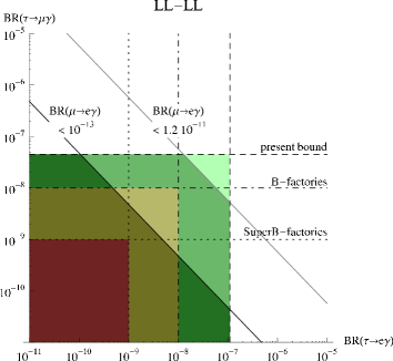
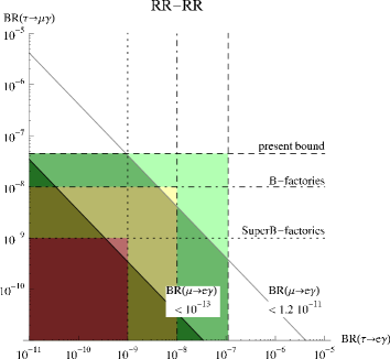
Figure 1: Allowed values for the branching ratios of the rare tau decays $\tau\rightarrow e\gamma$ and $\tau\rightarrow\mu\gamma$ from present experiments and from the bound ${\rm BR}(\mu\rightarrow e\gamma)\lower 2.71246pt\hbox{$\;\stackrel{{\scriptstyle\textstyle>}}{{\sim}}\;$}C\times{\rm BR}(\tau\rightarrow\mu\gamma){\rm BR}(\tau\rightarrow e\gamma)$ for the mass insertions falling in Class I (see text). The area in green indicates the values of the branching ratios that are accessible to present $B$-factories, and in yellow, the ones accessible to future super$B$-factories. Excluded regions are shown with light shading, whereas allowed regions are shown with dark shading. The supersymmetric benchmark point SPS1a has been assumed.

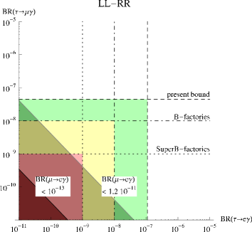
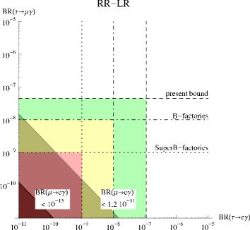
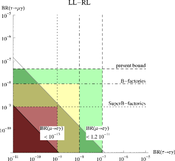
Figure 2: The same as Fig.1 but for Class II.

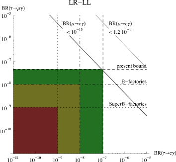
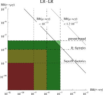
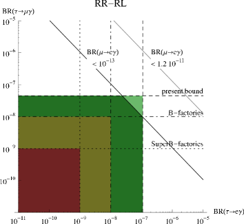
Figure 3: The same as Fig.1 but for Class III.

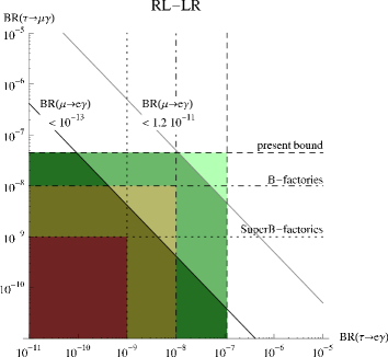
Figure 4: The same as Fig.1 but for Class IV.

The bounds Eqs.(11-14) also have implications for future searches for rare tau decays. In Figs. 1-4 we show with a dash-dotted line the projected sensitivity of present $B$-factories to rare tau decays (${\rm BR}(\tau\rightarrow\mu\gamma),{\rm BR}(\tau\rightarrow e\gamma)\lower 3.01385pt\hbox{$\;\stackrel{{\scriptstyle\textstyle>}}{{\sim}}\;$}10^{-8}$). Then, the area shaded in green is the region of this parameter space accessible to present $B$-factories. We find that for Class II the region where both $\tau\rightarrow\mu\gamma$ and $\tau\rightarrow e\gamma$ could be discovered at present $B$-factories is excluded. Therefore, if present $B$-factories discovered both rare tau decays, only supersymmetric models falling in Classes III, IV and Class I (for the case with LL-LL mass insertions) would be allowed. This conclusion will be strengthened if the MEG experiment at PSI reaches the projected sensitivity ${\rm BR}(\mu\rightarrow e\gamma)\sim 10^{-13}$ without finding a positive signal. If this is the case, the observation of both tau rare decays at present $B$-factories would point to an origin of the tau flavour violation falling only in Class III. The same rationale could be applied to the future searches of rare tau decays at the projected super$B$-factories. In Figs.  1-4 we also show as a yellow shaded area the region of the parameter space accessible to the projected super$B$-factories (${\rm BR}(\tau\rightarrow\mu\gamma),{\rm BR}(\tau\rightarrow e\gamma)\lower 3.01385pt\hbox{$\;\stackrel{{\scriptstyle\textstyle>}}{{\sim}}\;$}10^{-9}$). Whereas the present bound on $\mu\rightarrow e\gamma$ only has implications for the projected super$B$-factories for the models falling in Class II, if the bound on $\mu\rightarrow e\gamma$ is improved to the level of $10^{-13}$ our results will also be relevant for the models falling in Classes I and IV.

It is interesting to note that two of the most widely studied scenarios generating sizable rates for the rare decays, namely the supersymmetric see-saw model and the minimal SU(5) grand unified model, fall in Class I. To be precise, the supersymmetric see-saw model generates flavour violation in the LL sector [15] and the minimal SU(5) model, in the RR sector [16]. For Class I the bound Eq.(11) is quite stringent and disfavours the possibility of observing both rare tau decays at present $B$-factories for a generic point of the mSUGRA parameter space. Furthermore, the bounds derived in this paper for the MSSM are conservative and typically become more stringent as the physics that generates the flavour violation is specified. Indeed, as was shown in [9], two loop effects induced by right-handed neutrinos in the supersymmetric see-saw model generate the off-diagonal terms $({{\bf m}_{L}^{2}})_{12}$, $({{\bf A}_{e}})_{12}$ and $({{\bf A}_{e}})_{21}$, which contribute through a single mass insertion to ${\rm BR}(\mu\rightarrow e\gamma)$ in addition to the double mass insertion contribution considered in the present work.

To finish this section, let us review other theoretical constraints on the rare tau decays that have been derived in the literature for the MSSM. Interesting bounds on the branching ratios of the rare lepton decays were derived in [17] from requiring absence of charge breaking minima or unbounded from below directions in the effective potential. The respective resulting bounds on the LR and RL mass insertions read,

$$|\Delta^{\rm(LR)}_{ij}|,|\Delta^{\rm(RL)}_{ji}| \leq m_{k}\left[({{\bf m}_{e}^{2}})_{ii}+({{\bf m}_{L}^{2}})_{jj}+m_{H_{d}}^{2}\right]^{1/2}\;,$$

$$|\Delta^{\rm(LR)}_{ij}|,|\Delta^{\rm(RL)}_{ji}| \leq m_{k}\left[({{\bf m}_{e}^{2}})_{ii}+({{\bf m}_{L}^{2}})_{jj}+({{\bf m}_{L}^{2}})_{nn}\right]^{1/2},~{}~{}~{}~{}~{}n\neq i,j\;,$$ (19)

where $m_{k}$ is the lepton mass, $k={\rm Max}\ (i,j)$, and $m_{H_{d}}^{2}$ is the down-type Higgs mass squared. Substituting these bounds on the mass insertions in Eq.(9) one finally obtains the following approximate constraint on the radiative tau decays:

$${\rm BR}(\tau\rightarrow\l\gamma)\lower 3.01385pt\hbox{$\;\stackrel{{\scriptstyle\textstyle<}}{{\sim}}\;$}\frac{3\alpha^{3}}{G_{F}^{2}\widetilde{m}^{4}}\;{\rm BR}(\tau\rightarrow\l\nu_{\tau}\bar{\nu}_{\l})\sim 6\times 10^{-8}\left(\frac{\widetilde{m}}{400\,{\rm GeV}}\right)^{-4}\;,$$ (20)

which is comparable, for $\widetilde{m}\sim 400$ GeV, to the present experimental bounds on the rare tau decays. In particular, we obtain for the SPS1a (SPS1b) benchmark point, ${\rm BR}(\tau\rightarrow\l\gamma)\lower 3.01385pt\hbox{$\;\stackrel{{\scriptstyle\textstyle<}}{{\sim}}\;$}9\times 10^{-7}$ $(10^{-7})$ in the case of the LR mass insertion and ${\rm BR}(\tau\rightarrow\l\gamma)\lower 3.01385pt\hbox{$\;\stackrel{{\scriptstyle\textstyle<}}{{\sim}}\;$}9\times 10^{-7}$ $(2\times 10^{-7})$ for the case of the RL mass insertion.

If the origin of the lepton flavour violation in the rare tau decays could be pinpointed to the LR or the RL sector, the observation of $\tau\rightarrow\mu\gamma$ or $\tau\rightarrow e\gamma$ in the near future would set, following Eq.(20), an upper bound on the scalar masses, $\widetilde{m}\lower 3.01385pt\hbox{$\;\stackrel{{\scriptstyle\textstyle<}}{{\sim}}\;$}400$ GeV, in order to avoid the appearance of dangerous charge breaking minima or unbounded from below directions in the effective potential. Remarkably, the constraints on the rare tau decays derived in this paper could help to pinpoint the origin of the lepton flavour violation. As was argued before, if both $\tau\rightarrow e\gamma$ and $\tau\rightarrow\mu\gamma$ were observed in the near future, models falling in Class III, and possibly also in Class IV, would be favoured over models falling in Classes I and II, especially if the experimental bound on ${\rm BR}(\mu\rightarrow e\gamma)$ reaches the level of $10^{-13}$. Therefore, since models falling in Classes III or IV always involve a LR and/or a RL mass insertion, the bound Eq.(20) would apply at least for one of the rare decays, and accordingly an upper bound on the scalar masses would follow. Namely, if future experiments show that ${\rm BR}(\mu\rightarrow e\gamma)\leq 10^{-13}$ but ${\rm BR}(\tau\rightarrow\l\gamma)>10^{-8}$, it would follow that $\widetilde{m}\lower 3.01385pt\hbox{$\;\stackrel{{\scriptstyle\textstyle<}}{{\sim}}\;$}700$ GeV from requiring absence of charge breaking minima or unbounded from below directions in the effective potential.

3 The effective field theory approach

In this section we will derive, pursuing an effective field theory approach, a conservative bound on ${\rm BR}(\mu\rightarrow e\gamma)$ in terms of the branching ratios for the radiative tau decays. The resulting bound will be therefore completely model independent.

Our starting point is the electromagnetic transition amplitude for the processes $\tau\rightarrow\mu\gamma^{*}$ and $\tau\rightarrow e\gamma^{*}$, Eq. (1). If both transitions exist in Nature, the transition $\mu\rightarrow e\gamma^{*}$ will be automatically induced through the nine diagrams shown in Fig. 5. Among these, the diagrams (B3) and (C2) do not contribute to the dipole form factors $f_{M1}^{\mu e}$, $f_{E1}^{\mu e}$, which are the only ones that induce the process $\mu\rightarrow e\gamma$. On the other hand, since the photon circulating in the loop is off-shell, all the form factors that induce the electromagnetic tau transition (monopole and dipole) will contribute to $f_{M1}^{\mu e}$, $f_{E1}^{\mu e}$. However, in order to derive a bound of the form ${\rm BR}(\mu\rightarrow e\gamma)\lower 3.01385pt\hbox{$\;\stackrel{{\scriptstyle\textstyle>}}{{\sim}}\;$}C\times{\rm BR}(\tau\rightarrow\mu\gamma){\rm BR}(\tau\rightarrow e\gamma)$, we will be interested just in the contribution from the dipole operators, which are the only ones that induce the processes $\tau\rightarrow\mu\gamma$ and $\tau\rightarrow e\gamma$. We estimate that the dipole form factors satisfy the following relations:

$$\left|f_{M1}^{\mu e}\right| \;\stackrel{{\scriptstyle\textstyle>}}{{\sim}}\; \frac{9\alpha}{2\pi}\frac{m^{3}_{\tau}}{m_{\mu}}\left|f_{E1}^{\tau e*}f_{E1}^{\tau\mu}-f_{M1}^{\tau e*}f_{M1}^{\tau\mu}\right|\log\frac{\Lambda}{m_{\mu}}\;,$$

$$\left|f_{E1}^{\mu e}\right| \;\stackrel{{\scriptstyle\textstyle>}}{{\sim}}\; \frac{9\alpha}{2\pi}\frac{m^{3}_{\tau}}{m_{\mu}}\left|f_{E1}^{\tau e*}f_{M1}^{\tau\mu}-f_{M1}^{\tau e*}f_{E1}^{\tau\mu}\right|\log\frac{\Lambda}{m_{\mu}}\;,$$ (21)

from where it follows that

$${\rm BR}(\mu\rightarrow e\gamma) \;\stackrel{{\scriptstyle\textstyle>}}{{\sim}}\; \frac{1944\pi\alpha^{3}}{G_{F}^{2}}\frac{m^{6}_{\tau}}{m^{2}_{\mu}}\left[(|f_{E1}^{\tau\mu}|^{2}+|f_{M1}^{\tau\mu}|^{2})(|f_{E1}^{\tau e}|^{2}+|f_{M1}^{\tau e}|^{2})\right.$$ (22)

$$- \left.4{\rm Re}(f_{E1}^{\tau e}f_{M1}^{\tau e*}){\rm Re}(f_{E1}^{\tau\mu}f_{M1}^{\tau\mu*})\right]\log^{2}\frac{\Lambda}{m_{\mu}}\;,$$

being $\Lambda$ a cutoff. Assuming that each rare tau decay is dominated by just one of the dipole form factors, either the electric or the magnetic, one finally obtains

$${\rm BR}(\mu\rightarrow e\gamma) \;\stackrel{{\scriptstyle\textstyle>}}{{\sim}}\; \frac{27\,G_{F}^{2}\,\alpha}{128\,\pi^{5}}\frac{m^{6}_{\tau}}{m^{2}_{\mu}}\log^{2}\frac{\Lambda}{m_{\mu}}\frac{{\rm BR}(\tau\rightarrow\mu\gamma)}{{\rm BR}(\tau\rightarrow\mu\nu_{\tau}\bar{\nu}_{\mu})}\frac{{\rm BR}(\tau\rightarrow e\gamma)}{{\rm BR}(\tau\rightarrow e\nu_{\tau}\bar{\nu}_{e})}$$ (23)

$$\sim 4\times 10^{-23}\left(\frac{{\rm BR}(\tau\rightarrow\mu\gamma)}{4.5\times 10^{-8}}\right)\left(\frac{{\rm BR}(\tau\rightarrow e\gamma)}{1.1\times 10^{-7}}\right)\;,$$

where we have used $\Lambda=1$ TeV. The resulting bound is too weak to have any practical application, although it is has the theoretically interest of setting an absolute lower bound on ${\rm BR}(\mu\rightarrow e\gamma)$ in terms of the rare tau decays. As the fundamental theory that generates the effective dipole operators becomes specified, new contributions to the rare muon decay will typically arise, thus strengthening considerably the previous bound. This is the case in particular for the Minimal Supersymmetric Standard Model considered in the previous section: the one loop diagrams that induce the process $\mu\rightarrow e\gamma$ in the effective theory approach, Figs. 5, correspond to much more suppressed three loop diagrams once the complete theory has been specified.

(A1)

(A2)

(A3)

(B1)

(B2)

(B3)

(C1)

(C2)

(C3)

Figure 5: One loop Feynman diagrams that induce the process $\mu\rightarrow e\gamma$ from the effective operators that induce $\tau\rightarrow\mu\gamma$ and $\tau\rightarrow e\gamma$.

Using the same effective theory approach it is possible to compute also a lower bound on the branching ratio for the process $\mu\rightarrow e\gamma\gamma$, which is induced by the diagram shown in Fig. 6. The result is

$${\rm BR}(\mu\rightarrow e\gamma\gamma)\lower 3.01385pt\hbox{$\;\stackrel{{\scriptstyle\textstyle>}}{{\sim}}\;$}\frac{8m^{2}_{\mu}m^{2}_{\tau}\pi^{2}\alpha^{2}}{5G^{2}_{F}}\left[(|f_{E1}^{\tau\mu}|^{2}+|f_{M1}^{\tau\mu}|^{2})(|f_{E1}^{\tau e}|^{2}+|f_{M1}^{\tau e}|^{2})-4{\rm Re}(f_{E1}^{\tau e}f_{M1}^{\tau e*}){\rm Re}(f_{E1}^{\tau\mu}f_{M1}^{\tau\mu*})\right]\,.$$ (24)

As before, this bound can be rewritten in terms of the branching ratios of the radiative tau decays, yielding

$${\rm BR}(\mu\rightarrow e\gamma\gamma) \;\stackrel{{\scriptstyle\textstyle>}}{{\sim}}\; \frac{G_{F}^{2}m^{2}_{\mu}m^{2}_{\tau}}{5760\pi^{4}}\frac{{\rm BR}(\tau\rightarrow\mu\gamma)}{{\rm BR}(\tau\rightarrow\mu\nu_{\tau}\bar{\nu}_{\mu})}\frac{{\rm BR}(\tau\rightarrow e\gamma)}{{\rm BR}(\tau\rightarrow e\nu_{\tau}\bar{\nu}_{e})}$$ (25)

$$\sim 10^{-30}\left(\frac{{\rm BR}(\tau\rightarrow\mu\gamma)}{4.5\times 10^{-8}}\right)\left(\frac{{\rm BR}(\tau\rightarrow e\gamma)}{1.1\times 10^{-7}}\right)\;,$$

again far below the experimental upper bound, ${\rm BR}(\mu\rightarrow e\gamma\gamma)<7.2\times 10^{-11}$  [18].

Figure 6: Feynman diagram that induces the process $\mu\rightarrow e\gamma\gamma$ from the effective operators that induce $\tau\rightarrow\mu\gamma$ and $\tau\rightarrow e\gamma$.

4 Conclusions

We have derived in this paper theoretical constraints on the branching ratios of the rare tau decays of the form ${\rm BR}(\mu\rightarrow e\gamma)\lower 3.01385pt\hbox{$\;\stackrel{{\scriptstyle\textstyle>}}{{\sim}}\;$}C\times{\rm BR}(\tau\rightarrow\mu\gamma){\rm BR}(\tau\rightarrow e\gamma)$ in the Minimal Supersymmetric Standard Model and in a completely general setup, pursuing an effective field theory approach.

We have argued that in the MSSM the observation of both rare tau decays implies, barring cancellations, a non-vanishing rate for the process $\mu\rightarrow e\gamma$ through the double mass insertion in the slepton propagator. We have cataloged the sixteen possibilities for the double mass insertion in four classes, according to their dependence on $\tan\beta$, the fermion masses and the overall size of the scalar masses, which are the three parameters to which the constant $C$ is most sensitive to, and we have shown that for a wide class of models our bound constrains values for the branching ratios of the rare tau decays that are otherwise allowed by present experiments. We have shown that if present $B$-factories observe both $\tau\rightarrow\mu\gamma$ and $\tau\rightarrow e\gamma$, the underlying possible sources of flavour violation would be restricted to our Class III, and possibly Class IV, unless the supersymmetric parameters take special values. This conclusion would be strengthened if the MEG experiment at PSI reaches the sensitivity of $10^{-13}$ for ${\rm BR}(\mu\rightarrow e\gamma)$ without finding a positive signal. We have also discussed the complementarity of the constraints on the rare tau decays derived in this paper and the constraints stemming from requiring absence of charge breaking minima or unbounded from below directions in the effective potential.

Finally, we have derived for completeness theoretical constraints on the rare tau decay following an effective theory approach. The resulting bounds are too weak to have any practical interest, although they have the theoretical interest of setting absolute bounds on the rates of $\mu\rightarrow e\gamma$ and $\mu\rightarrow e\gamma\gamma$ in terms of the rates of $\tau\rightarrow\mu\gamma$ and $\tau\rightarrow e\gamma$.

References

• [1] R. Ammar et al. [CLEO Collaboration], Phys. Rev. Lett.  71 (1993) 674.
• [2] M. L. Brooks et al. [MEGA Collaboration], Phys. Rev. Lett.  83 (1999) 1521; M. Ahmed et al. [MEGA Collaboration], Phys. Rev.  D 65 (2002) 112002.
• [3] T. Mori et al. ”Search for $\mu\rightarrow e\gamma$ Down to $10^{-14}$ Branching Ratio”. Research Proposal to Paul Scherrer Institut. See also http://meg.web.psi.ch/
• [4] B. Aubert et al. [BABAR Collaboration], Phys. Rev. Lett.  96 (2006) 041801.
• [5] A. G. Akeroyd et al. [SuperKEKB Physics Working Group], arXiv:hep-ex/0406071; M. Bona et al., arXiv:0709.0451 [hep-ex].
• [6] K. Hayasaka et al. [Belle Collaboration], Phys. Lett.  B 666 (2008) 16.
• [7] S. L. Glashow, J. Iliopoulos and L. Maiani, Phys. Rev.  D 2 (1970) 1285.
• [8] S. M. Bilenkii, S. T. Petcov and B. Pontecorvo, Phys. Lett. B 67 (1977) 309; T. P. Cheng and L. Li, Phys. Rev. Lett. 45 (1980) 1908; W. J. Marciano and A. I. Sanda, Phys. Lett. B 67 (1977) 303; B. W. Lee, S. Pakvasa, R. E. Shrock and H. Sugawara, Phys. Rev. Lett. 38 (1977) 937 [Erratum-ibid. 38 (1977) 937].
• [9] A. Ibarra and C. Simonetto, JHEP 0804, 102 (2008).
• [10] S. Dimopoulos and H. Georgi, Nucl. Phys.  B 193 (1981) 150; J. R. Ellis and D. V. Nanopoulos, Phys. Lett.  B 110 (1982) 44; R. Barbieri and R. Gatto, Phys. Lett.  B 110 (1982) 211; M. J. Duncan, Nucl. Phys.  B 221 (1983) 285; J. F. Donoghue, H. P. Nilles and D. Wyler, Phys. Lett.  B 128, 55 (1983); A. Bouquet, J. Kaplan and C. A. Savoy, Phys. Lett.  B 148 (1984) 69; L. J. Hall, V. A. Kostelecky and S. Raby, Nucl. Phys.  B 267 (1986) 415.
• [11] J. Hisano, T. Moroi, K. Tobe and M. Yamaguchi, Phys. Rev.  D 53 (1996) 2442.
• [12] F. Gabbiani and A. Masiero, Nucl. Phys.  B 322 (1989) 235; J. S. Hagelin, S. Kelley and T. Tanaka, Nucl. Phys.  B 415 (1994) 293; D. Choudhury, F. Eberlein, A. Konig, J. Louis and S. Pokorski, Phys. Lett.  B 342 (1995) 180; B. de Carlos, J. A. Casas and J. M. Moreno, Phys. Rev.  D 53, 6398 (1996); F. Gabbiani, E. Gabrielli, A. Masiero and L. Silvestrini, Nucl. Phys.  B 477 (1996) 321; I. Masina and C. A. Savoy, Nucl. Phys.  B 661, 365 (2003); P. Paradisi, JHEP 0510 (2005) 006.
• [13] A. Czarnecki and E. Jankowski, Phys. Rev.  D 65 (2002) 113004.
• [14] B. C. Allanach et al., in Proc. of the APS/DPF/DPB Summer Study on the Future of Particle Physics (Snowmass 2001) ed. N. Graf, In the Proceedings of APS / DPF / DPB Summer Study on the Future of Particle Physics (Snowmass 2001), Snowmass, Colorado, 30 Jun - 21 Jul 2001, pp P125 [arXiv:hep-ph/0202233].
• [15] F. Borzumati and A. Masiero, Phys. Rev. Lett.  57 (1986) 961.
• [16] R. Barbieri and L. J. Hall, Phys. Lett.  B 338 (1994) 212; R. Barbieri, L. J. Hall and A. Strumia, Nucl. Phys.  B 445 (1995) 219.
• [17] J. A. Casas and S. Dimopoulos, Phys. Lett.  B 387 (1996) 107.
• [18] D. Grosnick et al., Phys. Rev. Lett.  57 (1986) 3241.