Dynamical Evolution of Interacting Modified Chaplygin Gas

Abstract

The cosmological model of the modified Chaplygin gas interacting with cold dark matter is studied. Our attention is focused on the final state of universe in the model. It turns out that there exists a stable scaling solution, which provides the possibility to alleviate the coincidence problem. In addition, we investigate the effect of the coupling constants $c_{1}$ and $c_{2}$ on the dynamical evolution of this model from the statefinder viewpoint. It is found that the coupling constants play a significant role during the dynamical evolution of the interacting MCG model. Furthermore, we can distinguish this interacting model from other dark energy models in the $s-r$ plane.

I I.  Introduction

There is increasing evidence that our universe is presently in a state of cosmic accelerating expansion phys1 . This result has been confirmed with observations via Supernovae Ia phys2 , Cosmic Microwave Background anisotropies phys3 , Large Scale Structure formation phys4 , baryon oscillations phys5 and weak lensing phys6 , etc. These observations strongly suggest that the universe is spatially flat and is dominated by an extra component with negative pressure, dubbed as dark energy phys7 ; phys8 . In the recent years, various candidates of dark energy have been proposed. The simplest candidate is the cosmological constant phys9 . But this scenario is plagued by the severe fine-tuning problem and the coincidence problem. Other possible forms of dark energy include quintessence phys10 , k-essence phys11 , phantom phys12 , Born-Infeld scalars phys13 , quintom phys14 , tachyon field phys15 , holographic dark energy phys16 , and so on. Additionally, the conjecture that dark energy and dark matter can be unified by using the so-called Chaplygin gas (CG) obeying an exotic equation of state (EoS)

$$p_{g}=-\frac{A}{\rho_{g}}$$ (1)

has been investigated in several literatures phys17 . Recently, the CG model was generalized to some possible forms phys18 . As an alternative model, the EoS of the generalized Chaplygin gas (GCG) phys19 reads

$$p_{g}=-\frac{A}{\rho_{g}^{\alpha}},$$ (2)

where $0\leq\alpha\leq 1$. It is clear that the case $\alpha=1$ corresponds to the CG. Within the framework of Friedmann-Robertson-Walker (FRW) cosmology, this EoS leads, after inserted into the relativistic energy conservation equation, to an energy density evolving as

$$\rho_{g}=(A+\frac{B}{a^{3(1+\alpha)}})^{\frac{1}{1+\alpha}},$$ (3)

where $B$ is an integration constant. Hence, we see that at early time the energy density behaves as a dust-like matter, while at late time it behaves like a cosmological constant. So the GCG model can also be interpreted as an entangled mixture of dark matter and dark energy. This dual role is at the heart of the surprising properties of the GCG model. However, these so-called unified dark matter models have been ruled out because they produce oscillations or exponential blowup of the matter power spectrum inconsistent with observation phys69 . But no observation so far rule out the possibility of the GCG as dark energy though it is disfavored as dark matter. In fact, the dynamical properties of the GCG have been studied in Ref. phys20 , which indicates that the EoS of the GCG may cross the so-called phantom divide $w=-1$ if there exists an interaction between the GCG and dark matter. Therefore, it is worthwhile to further understand such unified dark matter models by studying another candidate for the generalization of the CG, referred to as the modified Chaplygin gas (MCG) phys21 ; phys22 , which is characterized by a simple EoS

$$p_{g}=A\rho_{g}-\frac{B}{\rho_{g}^{\alpha}},$$ (4)

where $A$, $B$ and $\alpha$ are constants and $0\leq\alpha\leq 1$. The attractive feature of this model is that the EoS looks like that of two fluids, one obeying a perfect EoS $p=A\rho$ and the other being the GCG. From Eq. (4), it is easy to see that the MCG reduces to the GCG if $A=0$ and to the perfect fluid if $B=0$. Accordingly, the evolution of the energy density is given by

$$\rho_{g}=(\frac{B}{1+A}+\frac{C}{a^{3(1+A)(1+\alpha)}})^{\frac{1}{1+\alpha}},~{}~{}~{}~{}(A\neq-1)$$ (5)

where $C$ is the constant of integration. Thus the MCG behaves as a radiation (when $A=1/3$) or a dust-like matter (when $A=0$) at early stage, while as a cosmological constant at later stage.

As we all know, observations at the level of the solar system severely constrain non-gravitational interactions of baryons, namely, non-minimal coupling between dark energy and ordinary matter fluids is strongly restricted by the experimental tests in the solar systems phys23 . However, since the nature of dark sectors remains unknown, it is possible to have non-gravitational interactions between dark energy and dark matter. In this paper, we study the dynamical evolution of the interacting MCG model by considering an interaction term between the MCG and cold dark matter. In our scenario, we find that there exists a stable scaling solution, which is characterized by a constant ratio of the energy densities of the MCG and cold dark matter. This provides the possibility to alleviate the coincidence problem. Moreover, we find that the final state is determined by the parameters of the MCG, $\alpha$, $A$, and the coupling constants $c_{1}$ and $c_{2}$. The latter two parameters represent the transfer strength between the MCG and dark matter. Interestingly, we find that the EoS of the MCG $w_{g}$ tends to a constant, which is only determined by the coupling constants $c_{1}$ and $c_{2}$. However, both the EoS of the total cosmic fluid $w$ and the deceleration parameter $q$ tend to $-1$, which are independent of the choice of values for the parameters. This indicates that the cosmic doomsday is avoided and the universe enters to a de Sitter phase and thus accelerates forever. Further, we investigate the effect of the coupling constants $c_{1}$ and $c_{2}$ on the dynamical evolution of this model from the statefinder viewpoint. By our analysis, we see that the coupling cantants $c_{1}$ and $c_{2}$ play a significant role during the dynamics of the interacting MCG model. It is also worthwhile to note that, we can distinguish this interacting model from other dark energy models in the $s-r$ plane.

In Sec. II, we study the dynamical evolution of the interacting MCG. Then we apply the statefinder diagnosis to the interacting modified Chaplygin gas model for various different parameters in Sec. III. The conclusions are summarized in Sec. IV.

II II.  Dynamics analysis

In our scenario, the universe contains the MCG $\rho_{g}$ (as dark energy), cold dark matter $\rho_{m}$ and baryonic matter $\rho_{b}$. For a spatially flat universe, the Friedmann equation is

$$H^{2}=\frac{\kappa^{2}}{3}\rho=\frac{\kappa^{2}}{3}(\rho_{g}+\rho_{m}+\rho_{b}),$$ (6)

where $H$ is the Hubble parameter, $\kappa^{2}\equiv 8\pi G$ and $\rho$ is the total energy density (nature units $c=\hbar=1$ is used throughout the paper). Then differentiating the above equation with respect to cosmic time $t$ and using the total energy conservation equation

$$\dot{\rho}+3H(\rho+p)=0,$$ (7)

where $p$ is the total pressure of the background fluid, we can get the Raychaudhuri equation

$$\dot{H}=-\frac{\kappa^{2}}{2}(\rho_{g}+p_{g}+\rho_{m}+p_{b}),$$ (8)

in which $p_{g}$ represents the pressure of the MCG.

We postulate that the two dark sectors interact through the interaction term $Q$ and the baryonic matter only interacts gravitationally with the dark sectors. Then the continuity equation is written as

$$\dot{\rho}_{b}+3H(\rho_{b})=0,$$ (9)

$$\dot{\rho}_{m}+3H(\rho_{m})=Q,$$ (10)

$$\dot{\rho}_{g}+3H(\rho_{g}+p_{g})=-Q.$$ (11)

Clearly, $Q$ is the rate of the energy density exchange in the dark sectors and the sign of $Q$ determines the direction of energy transfer. A positive $Q$ corresponds to the transfer of energy from dark energy to dark matter, while a negative $Q$ represents the other way round. Due to the unknown nature of dark sectors, there is as yet no basis in fundamental theory for a special coupling between two dark sectors. So the interaction term $Q$ discussed currently has to be chosen in a phenomenological way phys40 . One possible choice for the interaction term is $Q=3H(c_{1}\rho_{m}+c_{2}\rho_{g})$ phys41 , where $c_{1}$ and $c_{2}$ are coupling constants. This form was first proposed in  phys42 and it is a more general form than those found in phys40 ; phys43 , which can be obtained when $c_{1}=c_{2}=c$, $c_{1}=0$ or $c_{2}=0$.

II.1 A.    Stability Analysis

To analyze the evolution of the dynamical system, we introduce the following dimensionless variables:

$$x\equiv\frac{\kappa^{2}\rho_{g}}{3H^{2}},~{}~{}~{}~{}~{}~{}~{}~{}y\equiv\frac{\kappa^{2}p_{g}}{3H^{2}},~{}~{}~{}~{}~{}~{}~{}~{}z\equiv\frac{\kappa^{2}\rho_{m}}{3H^{2}}.$$ (12)

Accordingly, the density of the baryonic matter is determined by the Friedmann constraint (6) as

$$\frac{\kappa^{2}\rho_{b}}{3H^{2}}=1-x-z,$$ (13)

which implies that $0\leq x+z\leq 1$ and $0\leq x,z\leq 1$. Furthermore, using these variables, the EoSs of the MCG and the total cosmic fluid are respectively given by

$$w_{g}=\frac{p_{g}}{\rho_{g}}=\frac{y}{x},$$ (14)

$$w=\frac{p}{\rho}=\frac{p_{g}}{\rho_{g}+\rho_{m}+\rho_{b}}=y.$$ (15)

The sound velocity and the deceleration parameter respectively read

$$c^{2}_{s}=\frac{\partial p_{g}}{\partial\rho_{g}}=-\alpha\frac{y}{x}+(1+\alpha)A,$$ (16)

$$q=-\frac{\ddot{a}a}{\dot{a}^{2}}=-1+\frac{3}{2}(1+y).$$ (17)

Note that the condition for acceleration is $w<-\frac{1}{3}$ and the physically meaningful range of the sound velocity is $0\leq c^{2}_{s}<1$. Using Eqs. (6)-(11), we can obtain the following autonomous system:

$$x^{{}^{\prime}} = -3[(1+c_{2})x+y+c_{1}z]+3x(1+y),$$ (18)

$$y^{{}^{\prime}} = -3[(1+c_{2})x+y+c_{1}z][-\alpha\frac{y}{x}+(1+\alpha)A]+3y(1+y),$$ (19)

$$z^{{}^{\prime}} = -3[-c_{2}x+(1-c_{1})z]+3z(1+y),$$ (20)

where the prime denotes a derivative with respect to $N\equiv lna$. We set the current scale factor by $a_{0}=1$. Then the current value of $N$ reads $N_{0}=0$. Setting $x^{{}^{\prime}}=y^{{}^{\prime}}=z^{{}^{\prime}}=0$, we can obtain the critical points $(x_{*},y_{*},z_{*})$ of the autonomous system as follows:

• point $(a)$:    ($\frac{A-c_{1}+c_{2}}{2A}(1+x_{s})$,  $\frac{A-c_{1}+c_{2}}{2}(1+x_{s})$,  $1-\frac{A-c_{1}+c_{2}}{2A}(1+x_{s})$),
  

• point $(b)$:    ($\frac{A-c_{1}+c_{2}}{2A}(1-x_{s})$,  $\frac{A-c_{1}+c_{2}}{2}(1-x_{s})$,  $1-\frac{A-c_{1}+c_{2}}{2A}(1-x_{s})$),
  

• point $(c)$:    ($\frac{1-c_{1}}{1-c_{1}+c_{2}}$,  $-1$,  $\frac{c_{2}}{1-c_{1}+c_{2}}$).

Here the parameter $x_{s}$ is defined by

$$x_{s}=\sqrt{1+\frac{4Ac_{1}}{(A-c_{1}+c_{2})^{2}}}.$$ (21)

Thus, we can constrain the parameters in the model under the physically meaningful conditions, namely, $0<x_{*}\leq 1$ and $0\leq c^{2}_{s*}<1$. Concretely, we analyze the existence conditions for these three points respectively:

$\bullet$ points $(a)$ and $(b)$: Considering the physically meaningful range of $x_{*}=\frac{A-c_{1}+c_{2}}{2A}(1\pm x_{s})$, we can obtain that $0<\frac{A-c_{1}+c_{2}}{2A}(1\pm x_{s})\leq 1,A\neq 0$, and moreover, $x_{s}$ is real. Together with the constraint of the sound velocity $c^{2}_{s*}=A$, namely, $0\leq A<1$, we can conclude that the existence conditions of points $(a)$ and $(b)$ are $c_{1}<0$, but $c_{1}\neq-1$, $-(1-\sqrt{-c_{1}})^{2}<c_{2}<0$ and $(\sqrt{-c_{1}}+\sqrt{-c_{2}})^{2}\leq A<1$.

$\bullet$ point $(c)$: According to the meaningful range of $x_{*}=\frac{1-c_{1}}{1-c_{1}+c_{2}}$, we know that $0<\frac{1-c_{1}}{1-c_{1}+c_{2}}\leq 1$, and therefore, $c{1}<1,c_{2}\geq 0$ or $c{1}>1,c_{2}\leq 0$. Furthermore, the constraint of the sound velocity $c^{2}_{s*}$ implies that the range of $A$ is $-\frac{\alpha}{1+\alpha}\frac{1-c_{1}+c_{2}}{1-c_{1}}\leq A<\frac{1}{1+\alpha}(1-\alpha\frac{1-c_{1}+c_{2}}{1-c_{1}})$. Thus, the existence conditions of point $(c)$ are obtained. Results from our above analysis are concluded in Table I.

Point	Existence	Eigenvalues	Stability	$w_{*}$	Acceleration
	$c_{1}<0$, but $c_{1}\neq-1$	$\lambda_{1}=3(A-c_{1}+c_{2})x_{s}$,
$(a)$	$-(1-\sqrt{-c_{1}})^{2}<c_{2}<0$	$\lambda_{2}=\frac{3}{2}(A-c_{1}+c_{2})(1+x_{s})$,	Unstable	$\frac{A-c_{1}+c_{2}}{2}(1+x_{s})$	No
	$(\sqrt{-c_{1}}+\sqrt{-c_{2}})^{2}\leq A<1$	$\lambda_{3}=3(1+\alpha)[1+\frac{(A-c_{1}+c_{2})}{2}(1+x_{s})]$
	$c_{1}<0$, but $c_{1}\neq-1$	$\lambda_{1}=-3(A-c_{1}+c_{2})x_{s}$,
$(b)$	$-(1-\sqrt{-c_{1}})^{2}<c_{2}<0$	$\lambda_{2}=\frac{3}{2}(A-c_{1}+c_{2})(1-x_{s})$,	Saddle	$\frac{A-c_{1}+c_{2}}{2}(1-x_{s})$	No
	$(\sqrt{-c_{1}}+\sqrt{-c_{2}})^{2}\leq A<1$	$\lambda_{3}=3(1+\alpha)[1+\frac{(A-c_{1}+c_{2})}{2}(1-x_{s})]$
			Stable if
			$c_{1}<1,c_{2}\geq 0$ and
	$c_{1}<1,c_{2}\geq 0$ or	$\lambda_{1}=-3$,	$-\frac{\alpha}{1+\alpha}\frac{1-c_{1}+c_{2}}{1-c_{1}}\leq A$
$(c)$	$c_{1}>1,c_{2}\leq 0$	$\lambda_{2,3}=-\frac{3}{2(c_{1}-1)}\{-\alpha(1-c_{1}+c_{2})$	$<\frac{1}{1+\alpha}(1-\alpha\frac{1-c_{1}+c_{2}}{1-c_{1}})$	$-1$	All
	$-\frac{\alpha}{1+\alpha}\frac{1-c_{1}+c_{2}}{1-c_{1}}\leq A$	$-(1-c_{1})[2-c_{1}+c_{2}+(1+\alpha)A]\pm\lambda_{s}\}$	Saddle if		$\alpha,A,c_{1}$ and $c_{2}$
	$<\frac{1}{1+\alpha}(1-\alpha\frac{1-c_{1}+c_{2}}{1-c_{1}})$		$c_{1}>1,c_{2}\leq 0$ and
			$-\frac{\alpha}{1+\alpha}\frac{1-c_{1}+c_{2}}{1-c_{1}}\leq A$
			$<\frac{1}{1+\alpha}(1-\alpha\frac{1-c_{1}+c_{2}}{1-c_{1}})$

Table 1: The properties of the critical points for the interacting modified Chaplygin gas model. Here, the parameter $\lambda_{s}$ is defined in Eq. (25).

To study the stability of the critical points for the autonomous system, we substitute linear perturbations $x\rightarrow x_{*}+\delta x$, $y\rightarrow y_{*}+\delta y$ and $z\rightarrow z_{*}+\delta z$ about the critical points into the autonomous system Eqs. (18)-(20). To first-order in the perturbations, one gets the following evolution equations of the linear perturbations:

$$\delta x^{{}^{\prime}} = 3(y_{*}-c_{2})\delta x+3(x_{*}-1)\delta y-3c_{1}\delta z,$$ (22)

$$\delta y^{{}^{\prime}} = -3[\alpha\frac{y_{*}}{x_{*}}(\frac{y_{*}}{x_{*}}+c_{1}\frac{z_{*}}{x_{*}})+(1+c_{2})(1+\alpha)A]\delta x$$ (23)

$$+3[1-(1+\alpha)A+(1+c_{2})\alpha+2y_{*}+\alpha(2\frac{y_{*}}{x_{*}}+c_{1}\frac{z_{*}}{x_{*}})]\delta y-3c_{1}[-\alpha\frac{y_{*}}{x_{*}}+(1+\alpha)A]\delta z,$$

$$\delta z^{{}^{\prime}} = 3c_{2}\delta x+3z_{*}\delta y+3(y_{*}+c_{1})\delta z.$$ (24)

The three eigenvalues of the coefficient matrix of Eqs. (22)-(24) determine the stability of the critical points. We list the three eigenvalues for each point in Table I. Moreover, the condition for stability and acceleration (i.e., $w_{*}<-\frac{1}{3}$) are also summarized in the same table. For convenience, we introduce the parameter

$$\lambda_{s}=\{[\alpha(1-c_{1}+c_{2})+(1+\alpha)(1-c_{1})A]^{2}+2(1-c_{1})(c_{1}+c_{2})[\alpha(1-c_{1}+c_{2})+(1+\alpha)(1-c_{1})A]+[(1-c_{1})(c_{1}-c_{2})]^{2}\}^{\frac{1}{2}}.$$ (25)

From Table I, we can clearly see that points $(a)$ and $(b)$ are not stable if they exist, and point $(c)$ is stable under conditions $c_{1}<1,c_{2}\geq 0$ and $-\frac{\alpha}{1+\alpha}\frac{1-c_{1}+c_{2}}{1-c_{1}}\leq A<\frac{1}{1+\alpha}(1-\alpha\frac{1-c_{1}+c_{2}}{1-c_{1}})$. Furthermore, the stable attractor is a scaling solution since the energy density of the MCG remains proportional to that of cold dark matter, $\frac{\rho_{g*}}{\rho_{m*}}=\frac{1-c_{1}}{c_{2}}$, when $c_{2}\neq 0$. Thus, point $(c)$ is an accelerated scaling solution that probably alleviates the coincidence problem. Additionally, for the stable attractor point $(c)$, the location of the point depends only on the coupling constant $c_{1}$ and $c_{2}$. The EoS of the total cosmic fluid reads $w_{*}=-1$, which indicates that point $(c)$ is a accelerated attractor ($w_{*}<-\frac{1}{3}$) and implies that the universe will enter to a de sitter phase and accelerate forever, and therefore, there is no singularity in the finite future for any parameters. However, the EoS of the MCG is expressed by $w_{g*}=-\frac{1-c_{1}+c_{2}}{1-c_{1}}=-1-\frac{c_{2}}{1-c_{1}}$, that is to say, point $(c)$ has a phantom equation of state ($w_{g*}<-1$) for $c_{1}<1,c_{2}\geq 0$. According to Eq. (17), we can obtain that $q_{*}=-1+\frac{3}{2}(1+y_{*})=-1$ for the stable attractor point $(c)$, which also implies that the universe will enter to a de sitter phase and accelerate forever.

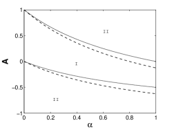
Figure 1: The stable regions in the $(\alpha,A)$ parameter space. The solid and dotted lines respectively denote the region for $c_{1}=c_{2}=0$ (the modified Chaplygin gas model without interaction) or $c_{1}\neq 0,c_{2}=0$ (coupling between dark sectors only proportional to the energy density of dark matter) and $c_{1}=c_{2}=0.2$. In the region I (the region between the two same lines), point $(c)$ is a stable accelerated attractor. The region II represents the region of solution without physical meaning.

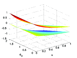
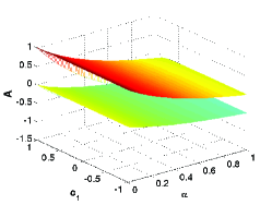
Figure 2: The stable regions in the parameter space for the fixed $c_{1}$ or $c_{2}$. The left two correspond to $c_{1}=0$ (coupling between dark sectors only proportional to the energy density of dark energy) and $c_{1}=0.4$, respectively. The right is for $c_{2}=0.02$. The region between the two colorful planes represents that point $(c)$ is a stable accelerated attractor. The other regions correspond to the regions of solution without physical meaning.

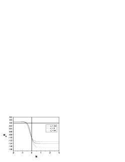
Figure 3: The evolution of the EoSs of the modified Chaplygin gas $w_{g}$ for different values of various parameters. The top two plots correspond to the cases for different values of the modified Chaplygin gas parameters $\alpha$ or $A$, when $c_{1}=0.2$ and $c_{2}=0.4$. In addition, we respectively fix the parameter $A=0.1$ and $\alpha=0.5$ in these two plots. The bottom two plots represent the case for different values of the coupling constants $c_{1}$ or $c_{2}$, when $\alpha=0.5$ and $A=0.1$. Moreover, in these two plots, the parameter $c_{2}$ and $c_{1}$ are fixed to be $c_{2}=0.4$ and $c_{1}=0.2$ respectively.

II.2 B.    Numerical Results

In what follows, we numerically study the dynamical results from the autonomous system (18)-(20) to clearly confirm the complicated stability condition for the stable accelerated attractor point $(c)$. In Figs.1 and 2, we depict the parameter space for point $(c)$ to be stable. We suppose that $c_{1}=c_{2}=c$ or $c_{1}\neq 0,c_{2}=0$ in Fig.1. From the figure, we see that the parameter space is independent of the coupling constant $c_{1}$ when $c_{2}=0$, namely, the stable region of the modified Chaplygin gas without interaction ($c_{1}=c_{2}=0$) is the same as that of the interacting MCG, in which the interaction term is solely proportional to the energy density of dark matter ($c_{1}\neq 0,c_{2}=0$). Fig.2 shows that the stable regions in the parameter space for the fixed $c_{1}$ or $c_{2}$. In the figure, the left two plots is respectively for $c_{1}=0$ and $c_{1}=0.4$, meanwhile, the range of $c_{2}$ is specially chosen as $0\leq c_{2}<2$ to present the results more transparently though $c_{2}\geq 0$ is permitted. The right plot is shown by choosing $c_{2}=0.02$, and also the range of $c_{1}$ is selected as $-1\leq c_{1}<1$ for clarity although its allowed range is $c_{1}<1$.

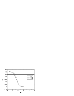
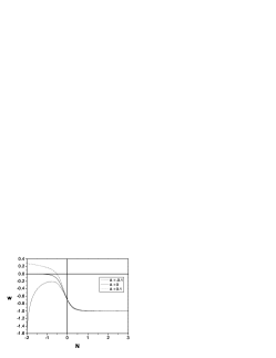
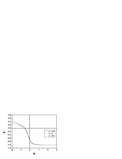
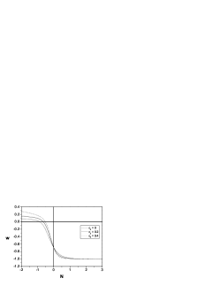
Figure 4: The evolution of the EoSs of the total cosmic fluid $w$ for different values of various parameters. In these four plots, we respectively select the same parameters as those in Fig.3.

In Figs.3-4, we plot the evolution of the EoSs of the MCG $w_{g}$ and the total cosmic fluid $w$ for different parameters in the stable region to illustrate the evolutional feature of our universe. Meanwhile, the initial condition in these figures is taken to be $x_{0}=\Omega_{g0}=0.7$, $y_{0}=-0.7$ (we assume $w_{g0}=-1$) and $z_{0}=\Omega_{mo}=0.26$ to compare with the observation data. As example, we choose several sets of values for the parameters $\alpha$, $A$, $c_{1}$ and $c_{2}$ for clarity. From Fig.3, we see that in the final state the EoS of the MCG, $w_{g}$, tends to a constant, which is only determined by the coupling constants $c_{1}$ and $c_{2}$. Furthermore, the final EoS of the MCG, $w_{g*}$, is always below $-1$ for different parameters in the stable region, i.e., the MCG has a phantom equation of state in the final state. In Fig.4, we find that the final EoS of the total cosmic fluid $w_{*}$ tends to $-1$, which is independent of any parameters in the stable region. This indicates that the cosmic doomsday is avoided and the universe accelerates forever. Note that the evolution of $w$ is exotic when a set of parameters is chosen as $\alpha=0.5$, $A=-0.1$, $c_{1}=0.2$ and $c_{2}=0.4$. In this case, the value of $w$ is smaller than $-1$ at the high redshift, i.e., the interacting modified Chaplygin gas model behave as phantom ($w<-1$) at the not very early universe.

As the most significant parameter from the viewpoint of observations, the deceleration parameter $q$ is also discussed. We exhibit the evolution of the deceleration parameter $q$ for various parameters in the stable region in Fig.5. The sets of values for all parameters in this model are selected as those in Fig.3-4. From the figure, we find that in the final state the deceleration parameter $q$ tends to $-1$ for different values of various parameters. This further indicates the universe enters to a de Sitter phase in the final state. Moreover, varying any one of the MCG parameters $\alpha$, $A$ and the coupling constants $c_{1}$, $c_{2}$, and fixing the rest, we find that the larger the variational parameter is, the smaller the transition redshift $z_{t}$ is, namely, the later the transition from the deceleration phase to the acceleration phase is. In addition, it is worthwhile to note that when we fix the parameters $\alpha=0.5$, $c_{1}=0.2$ and $c_{2}=0.4$, and select $A=-0.1$, there are two transition redshift: the first one denotes the transition from the acceleration phase to the deceleration phase; the second one represents the transition point from the deceleration phase to the acceleration phase. This provides the possibility that the evolution of our universe from acceleration to deceleration and then from deceleration to acceleration.

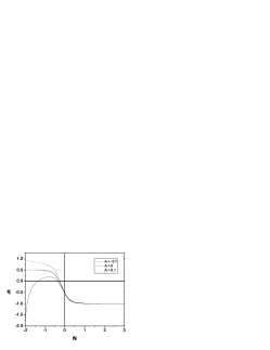
Figure 5: The evolution of the deceleration parameter $q$ for different values of various parameters. Also, the parameters in these four plots are respectively chosen as those in Fig.3 for clarity.

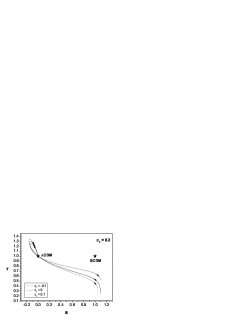
Figure 6: The evolution of the statefinder for the interacting MCG model in the $s-r$ plane with different coupling constants $c_{1}$ and $c_{2}$, which is illustrated in the left one and the right two panels, respectively. To be clarity, we extract a part of the middle panel to be the right one. In these three plots, we fix the parameters $\alpha=0.5$ and $A=-0.1$. The solid points show the current values of the statefinder parameters $(s_{0},r_{0})$.

III III.  STATEFINDER DIAGNOSIS

In this section, we study the dynamics of the interacting modified Chaplygin gas model from the statefinder viewpoint. The so-called statefinder parameter was first introduced by Sahni et al. phys44 in order to discriminate among more and more cosmological models. It is constructed from the scalar $a$ and its derivatives up to the third order. The statefinder pair $\{r,s\}$ is defined as

$$r\equiv\frac{\dddot{a}}{aH^{3}},\mbox{}\hskip 15.0pts\equiv\frac{r-1}{3(q-1/2)}.$$ (26)

Since different cosmological models exhibit qualitatively different trajectories of evolution in the $s-r$ plane, the statefinder parameter is a good tool to distinguish cosmological models. It has a remarkable property for the basic spatially flat $\Lambda$CDM model and the matter dominated universe SCDM, i.e., the statefinder pair $\{r,s\}$ for $\Lambda$CDM model takes the constant value $(0,1)$, while SCDM model corresponds to the fixed point $(1,1)$. We can clearly identify the “distance” from a given cosmological model to $\Lambda$CDM model in the $s-r$ plane, such as the quintessence, the phantom, the Chaplygin gas, the holographic dark energy models, the interacting dark energy models, and so forth, which have been shown in the literatures phys45 .

Generally, according to the reexpression of the deceleration parameter $q$

$$q=-1-\frac{\dot{H}}{H},$$ (27)

we can also rewrite the statefinder pair $\{r,s\}$ in terms of the Hubble parameter $H$ and its first and second derivatives with respect to the cosmic time $t$, $\dot{H}$ and $\ddot{H}$, as

$$r = 1+3\frac{\dot{H}}{H^{2}}+\frac{\ddot{H}}{H^{3}},$$ (28)

$$s =- \frac{3\frac{\dot{H}}{H^{2}}+\frac{\ddot{H}}{H^{3}}}{3(\frac{\dot{H}}{H^{2}}+\frac{3}{2})}.$$ (29)

Now we apply the statefinder parameter to the interacting MCG model. By using Eqs. (6)-(11), the statefiner parameter can be concretely expressed as

$$r = 1+\frac{9}{2}[(1+c_{2})x+y+c_{1}z][-\alpha\frac{y}{x}+(1+\alpha)A],$$ (30)

$$s = \frac{[(1+c_{2})x+y+c_{1}z][-\alpha\frac{y}{x}+(1+\alpha)A]}{y}.$$ (31)

The evolution of statefinder for the interacting MCG model in the $s-r$ plane is plotted in Fig.6. The arrows in the figure denote the evolution directions of the statefinder trajectories. In this figure, we also use the initial condition: $x_{0}=\Omega_{g0}=0.7$, $y_{0}=-0.7$ (we assume $w_{g0}=-1$) and $z_{0}=\Omega_{mo}=0.26$. Since the evolution trajectory in the $s-r$ plane will be interrupted when $y=0$ (i.e.,$w=0$), which is not our favorite case, we carefully choose the parameter $A=-0.1$ based on the model parameters selected before to avoid the interruption. This choice can be seen from Fig.4, in which we can avoid the possibility of $w=0$ during its evolution only if $A\geq 0$ based on the model parameters we selected. So in Fig.6, we take $A=-0.1$ and $\alpha=0.5$ as example to investigate the effect of the coupling constants $c_{1}$ and $c_{2}$, and furthermore, to discriminate between the interacting MCG model and other dark energy models. From Fig.6, we see that the evolution trajectories not only cross the $\Lambda$CDM fixed point but also end at the fixed point for various values of $c_{1}$ and $c_{2}$. However, the $r(s)$ curve could not traverse the SCDM fixed point for any case. In addition, in the left plot, the $r(s)$ curves are very different with various $c_{1}$ and the fixed $c_{2}$, especially, the current values of $(s,r)$ are different for various values of $c_{1}$. Also, we can clearly see the tremendous difference between the current values $(s_{0},r_{0})$ and the $\Lambda$CDM fixed point, and the larger the value of $c_{1}$ is, the greater the “distance” from the current value $(s_{0},r_{0})$ to the fixed point is. On the other hand, fixing the coupling constant $c_{1}$ and varying $c_{2}$ as illustrated in the right two plots of Fig.6, we find that the $r(s)$ curves are very different from each other with various $c_{2}$, and the current values of $(s,r)$ are distinct for different values of $c_{2}$. Also, we can clearly see the difference between the current values $(s_{0},r_{0})$ and the $\Lambda$CDM fixed point, and the larger the value of $c_{2}$ is, the greater the “distance” from $(s_{0},r_{0})$ to the fixed point is. Therefore, we can conclude that the statefinder diagnosis can not only discriminate the interacting MCG model with different coupling constant but also distinguish the interacting MCG model from other dark energy models.

IV IV.  Conclusions

In previous sections, we have studied some physical properties of the interacting MCG model. By considering an interaction term between the MCG and cold dark matter, we study the dynamical evolution of this model and pay our attention to the final state of the universe. By our analysis, there exists a stable scaling solution, which is characterized by a constant ratio of the energy densities of the MCG and dark matter. This provides the possibility to alleviate the coincidence problem. Furthermore, we see that the final state is determined by the parameters of the MCG $\alpha$, $A$ and the coupling constants $c_{1}$ and $c_{2}$.

Interestingly, we find that the EoS of the MCG, $w_{g}$, tends to a constant, which is only determined by the coupling constants $c_{1}$ and $c_{2}$. But both the EoS of the total cosmic fluid $w$ and the deceleration parameter $q$ tend to $-1$, which are independent of the choice of values for the parameters. This indicates that the cosmic doomsday is avoided and the universe enters to a de Sitter phase and thus accelerates forever. The transition from the deceleration phase to the acceleration phase also depends on the MCG parameters $\alpha$, $A$ and the coupling constants $c_{1}$, $c_{2}$. Varying one of these four parameters and fixing the rest, we find that the the larger the variational parameter is, the smaller the transition redshift $z_{t}$ is, namely, the later the transition from the deceleration phase to the acceleration phase is. Further, we study the effect of the coupling constants $c_{1}$ and $c_{2}$ on the dynamical evolution of this model from the statefinder viewpoint. We clearly see that the coupling constants $c_{1}$ and $c_{2}$ play a significant role during the dynamics of the interacting MCG model. The evolution trajectories of the statefinder for the interacting MCG model not only cross the $\Lambda$CDM fixed point but also end at the fixed point for various values of $c_{1}$ and $c_{2}$. However, the $r(s)$ curve could not traverse the SCDM fixed point for any case. Moreover, fixing one of the coupling constants $c_{1}$ and $c_{2}$, and varying the other one, we find that the larger the variational parameter is, the greater the “distance” from the current value $(s_{0},r_{0})$ to the fixed point is. Thus, the statefinder parameter can discriminate the interacting MCG model with different coupling constant. It is also worthwhile to note that, we can distinguish this interacting model from other dark energy models in the $s-r$ plane.

V Acknowledgements

This work is a part of project 10675019 supported by NSFC.

References

- (1) S. Perlmutter et al., Nature391,51 (1998); A.G. Riess et al., Astron. J.117,707 (1999); T. Padmanabhan, Phys. Rept.380,235 (2003).
- (2) J.L. Tonry et al., Astrophys. J.594,1 (2003); R.A. Knop et al., Astrophys. J.598,102 (2003).
- (3) D. N. Spergel et al., Astrophys. J. Suppl.148,175 (2003); C. L. Bennett et al., Astrophys. J. Suppl.148,1 (2003); S. Masi et al., Prog. Part. Nucl. Phys.48,243 (2002).
- (4) M. Tegmark et al., Phys. Rev. D69,103501 (2004); K. Abazajian et al., Astrophys. J.128,502 (2004); U. Seljak et al., Phys. Rev. D71,103515 (2005).
- (5) D.J. Eisenstein et al., Astrophys. J.633,560 (2005); C. Blake, D. Parkinson, B. Bassett, K. Glazebrook, M. Kunz and R.C. Nichol, Mon. Not. Roy. Astron. Soc.365, 255 (2006).
- (6) B. Jain and A. Taylor, Phys. Rev. Lett91,141302 (2003).
- (7) A.G. Riess et al., Astrophys. J.116,1009 (1998); P.M. Garnavich et al., Astrophys. J.493,L53 (1998); S. Perlmutter et al., Astrophys. J.517,565 (1999).
- (8) B.J. Barris et al., Astrophys. J.602,571 (2004); A.G. Riess et al., Astrophys. J.607,665 (2004); C.L. Bennett et al., Astrophys. J. Suppl.148,1 (2003).
- (9) S.M. Carroll, Living Rev. Rel.4,1 (2001); P.J.E. Peebles and B. Ratra, Rev. Mod. Phys.75,559 (2003).
- (10) I. Zlatev, L.M. Wang and P.J. Steinhardt, Phys. Rev. Lett82,896 (1999); P.J. Steinhardt, L.M. Wang and I.Zlatev, Phys. Rev. D59,123504 (1999).
- (11) C. Armendariz-Picon, V.F. Mukhanov and P.J. Steinhardt, Phys. Rev. Lett85,4438 (2000); T. Chiba, T. Okabe and M. Yamaguchi, Phys. Rev. D62,023511 (2000); C. Armendariz-Picon, V.F. Mukhanov and P.J. Steinhardt, Phys. Rev. D63,103510 (2001).
- (12) R.R. Caldwell, Phys. Lett. B545,23 (2002); R.R. Caldwell, M. Kamionkowski and N.N. Weinberg, Phys. Rev. Lett91,071301 (2003).
- (13) G.W. Gibbons, Phys. Lett. B537,1 (2002); T. Padmanabhan, Phys. Rev. D,66,021301 (2002); J.S. Bagla, H.K. Jassal and T. Padmanabhan, Phys. Rev. D67,063504 (2003).
- (14) B. Feng, X.L. Wang and X.M. Zhang, Phys. Lett. B607,35 (2005); X. Zhang, Commun. Theor. Phys.,762 (2005).
- (15) A. Frolov, L. Kofman and A. Starobinsky, Phys. Lett. B545,8 (2002); M. Fairbairn and M.H.G. Tytgat, Phys. Lett. B546,1 (2002); Y.S. Piao, R.G. Cai, X. Zhang and Y.Z. Zhang, Phys. Rev. D66,121301 (2002).
- (16) M. Li, Phys. Lett. B603,1 (2004); Y. Gong, Phys. Rev. D70,064029 (2004); X. Zhang and F.G. Wu, Phys. Rev. D72,043524 (2005).
- (17) A.Y. Kamenshchik, U. Moschella and V. Pasquier, Phys. Lett. B511,265 (2001); M.C. Bento et al., Phys. Rev. D70,083519 (2004); H.S. Zhang and Z.H. Zhu, Phys. Rev. D73,043518 (2006).
- (18) N. Bilic, G.B. Tupper and R.D. Viollier, Phys. Lett. B535,17 (2002); L.P. Chimento, Phys. Rev. D69,123517 (2004); X. Zhang, F.Q. Wu and J.F. Zhang, JCAP0601,003 (2006).
- (19) M.C. Bento, O. Bertolami and A.A. Sen, Phys. Rev. D66,043507 (2002).
- (20) H. Sandvik, M. Tegmark, M. Zaldarriaga and I. waga, Phys. Rev. D69,123524 (2004).
- (21) J.G. Hao and X.Z. Li, Phys. Lett. B606,7 (2005); P.X. Wu and H.W. Yu, Class. Quant. Grav.24,4661 (2007).
- (22) H.B. Benaoum, Accelerated Universe from Modified Chaplygin Gas and Tachyonic Fluid, arXiv: hep-th/0205140; L.P. Chimento and R. Lazkoz, Phys. Lett. B615,17 (2005); U. Debnath, A. Banerjee and S. Chakraborty, Class. Quant. Grav.21,5609 (2004).
- (23) M. Jamil and M.A. Rashid, Constraints on Coupling Constant Between Chaplygin Gas and Dark Matter, arXiv: astro-ph/08021144.
- (24) C.M. Will, Living Rev. Rel.4,4 (2001).
- (25) W. Zimdahl, D. Pavon and L.P. Chimento, Phys. Lett. B521,133 (2001); L.P. Chimento, A.S. Jakubi, D. Pavon and W. Zimdahl, Phys. Rev. D67,083513 (2003).
- (26) M. Quartin, M.O. Calvao, S.E. Joras, R.R.R. Reis, and I. Waga, JCAP0805,007 (2008); G.C. Cabral, R. Maartens amd L.A.U. Lopez, Phys. Rev. D79,063518 (2009).
- (27) H.M. Sadjadi and M. Alimohammadi, Phys. Rev. D 74,103007 (2006).
- (28) L. Amendola, Phys. Rev. D62,043511 (2000); W. Zimdahl, Int. J. Mod. Phys. D14,2319 (2005); D. Pavon and W. Zimdahl, Phys. Lett. B628,206 (2005);Z.K. Guo, N. Ohta and S. Tsujikawa, Phys. Rev. D 76,023508 (2007); L. Amendola, G.C. Campos, R. Rosenfeld, Phys.Rev.D75,083506 (2007); D. Pavon and B. Wang, Gen. Rel. Grav.41,1 (2009).
- (29) V. Sahni, T.D. Saini, A.A. Starobinsky and U. Alam,:JETP Lett.77, 201 (2003).
- (30) U. Alam, V. Sahni, T.D. Saini and A.A. Starobinsky, Mon. Not. Roy. Astron. Soc. 344, 1057 (2003); X. Zhang, Phys. Lett. B 611, 1 (2005); X. Zhang, Int. J. Mod. Phys. D 14, 1597 (2005); P.X. Wu and H.W. Yu, Int. J. Mod. Phys. D 14, 1873 (2005); B.R. Chang, H.Y. Liu, L.X. Xu, C.W. Zhang and Y.L. Ping, JCAP 0701, 016 (2007); M.R. Setare, J.F. Zhang and X. Zhang, JCAP 0703, 007 (2007); Z.L. Yi and T.J. Zhang, Phys. Rev. D 75, 083515 (2007); H. Wei, R.G. Cai, Phys. Lett. B 655, 1 (2007); J.F. Zhang, X. Zhang and H.Y. Liu, Phys. Lett. B 659, 26 (2008); D.J. Liu, W.Z. Liu, Phys. Rev. D 77, 027301 (2008).