Model-Independent Distance Measurements from Gamma-Ray Bursts
and Constraints on Dark Energy

Abstract

Gamma-Ray Bursts (GRB) are the most energetic events in the Universe, and provide a complementary probe of dark energy by allowing the measurement of cosmic expansion history that extends to redshifts greater than 6. Unlike Type Ia supernovae (SNe Ia), GRBs must be calibrated for each cosmological model considered, because of the lack of a nearby sample of GRBs for model-independent calibration. For a flat Universe with a cosmological constant, we find $\Omega_{m}=0.25^{+0.12}_{-0.11}$ from 69 GRBs alone. We show that the current GRB data can be summarized by a set of model-independent distance measurements, with negligible loss of information. We constrain a dark energy equation of state linear in the cosmic scale factor using these distance measurements from GRBs, together with the “Union” compilation of SNe Ia, WMAP five year observations, and the SDSS baryon acoustic oscillation scale measurement. We find that a cosmological constant is consistent with current data at 68% confidence level for a flat Universe. Our results provide a simple and robust method to incorporate GRB data in a joint analysis of cosmological data to constrain dark energy.

I Introduction

Gamma-ray bursts (GRBs) are the most luminous astrophysical events observable today, because they are at cosmological distances Paczynski95 . The duration of a gamma-ray burst is typically a few seconds, but can range from a few milliseconds to several minutes. The initial burst at gammay-ray wavelengths is usually followed by a longer-lived afterglow at longer wavelengths (X-ray, ultraviolet, optical, infrared, and radio). Gamma-ray bursts have been detected by orbiting satellites about two to three times per week. Most observed GRBs appear to be collimated emissions caused by the collapse of the core of a rapidly rotating, high-mass star into a black hole. A subclass of GRBs (the “short” bursts) appear to originate from a different process, the leading candidate being the collision of neutron stars orbiting in a binary system. See Ref.Meszaros06 for a recent review on GRBs.

GRBs can be used as distance indicators GRBde , thus provide a complementary probe of dark energy. The main advantage of GRBs over Type Ia Supernovae (SNe Ia) is that they span a much greater redshift range (from low $z$ to $z>6$). The main disadvantage is that GRBs have to be calibrated for each cosmological model tested (see for example, Ref.Schaefer04 ). This is in contrast to SNe Ia, where the calibration relations are established using nearby SNe Ia, and applied to high $z$ SNe Ia to extract cosmological constraints. There are no nearby GRBs that can be used for calibration. Thus, the GRB data must be fitted simultaneously for calibration and cosmological parameters. This makes the use of GRBs to probe cosmology somewhat cumbersome.

In this paper we show that the current GRB data can be summarized by a set of model-independent distance measurements. Our results provide an easy, robust, and transparent way to incorporate GRB data in an analysis of combined cosmological data to constrain dark energy.

II Method

II.1 Calibration of GRBs

Following Schaefer07 , we consider five calibration relations for GRBs. These relate GRB luminosity, $L$, or the total burst energy in the gamma rays, $E_{\gamma}$, to observables of the light curves and/or spectra: $\tau_{\mathrm{lag}}$ (time lag), $V$ (variability), $E_{\mathrm{peak}}$ (peak of the $\nu F_{\nu}$ spectrum), and $\tau_{\mathrm{RT}}$ (minimum rise time):

$$\log\left(\frac{L}{1\;\mathrm{erg}\;\mathrm{s}^{-1}}\right) = a_{1}+b_{1}\log\left[\frac{\tau_{\mathrm{lag}}(1+z)^{-1}}{0.1\;\mathrm{s}}\right],$$ (1)

$$\log\left(\frac{L}{1\;\mathrm{erg}\;\mathrm{s}^{-1}}\right) = a_{2}+b_{2}\log\left[\frac{V(1+z)}{0.02}\right],$$ (2)

$$\log\left(\frac{L}{1\;\mathrm{erg}\;\mathrm{s}^{-1}}\right) = a_{3}+b_{3}\log\left[\frac{E_{\mathrm{peak}}(1+z)}{300\;\mathrm{keV}}\right],$$ (3)

$$\log\left(\frac{E_{\gamma}}{1\;\mathrm{erg}}\right) = a_{4}+b_{4}\log\left[\frac{E_{\mathrm{peak}}(1+z)}{300\;\mathrm{keV}}\right],$$ (4)

$$\log\left(\frac{L}{1\;\mathrm{erg}\;\mathrm{s}^{-1}}\right) = a_{5}+b_{5}\log\left[\frac{\tau_{\mathrm{RT}}(1+z)^{-1}}{0.1\;\mathrm{s}}\right].$$ (5)

Not surprisingly, $E_{\mathrm{peak}}$ carries the most distance information. The $E_{\mathrm{peak}}$ – $E_{\gamma}$ relation is the tightest of the GRB calibration relations. To be included in this relation, the GRB afterglow must have an observed jet break in its light curve, and this means that only a fraction of GRBs with redshifts can contribute to establishing this relation. The variability-luminosity relation has the largest scatter. The variability is a measure of the sharpness of the pulse structure, which is determined by the size of the visible region in the jet.

In order to calibrate GRBs, $L$ and $E_{\gamma}$ must be related to the observed bolometric peak flux, $P_{\mathrm{bolo}}$, and the bolometric fluence, $S_{\mathrm{bolo}}$:

$$L = 4\pi d_{L}^{2}P_{\mathrm{bolo}}$$

$$E_{\gamma} = E_{\gamma,\mathrm{iso}}F_{\mathrm{beam}}=4\pi d_{L}^{2}S_{\mathrm{bolo}}(1+z)^{-1}F_{\mathrm{beam}},$$ (6)

where $E_{\gamma,\mathrm{iso}}$ is the isotropic energy. Clearly, the calibration of GRBs depend on the cosmological model through the luminosity distance $d_{L}(z)$.

The cosmological constraints from GRBs are sensitive to how the GRBs are calibrated. Calibrating GRBs using Type Ia supernovae (SNe Ia) gives tighter constraints than calibrating GRBs internally Liang08 . In this paper, we choose to calibrate GRBs internally, without using any external data sets, so that our results can be used to combine with any other cosmological data sets.

In fitting the five calibration relations, we need to fit a data array $\{x_{i},y_{i}\}$ with uncertainties $\{\sigma_{x,i},\sigma_{y,i}\}$, to a straight line

$$y=a+bx$$ (7)

through the minimization of $\chi^{2}$ given by Press07

$$\chi^{2}=\sum_{i=1}^{N}\frac{\left(y_{i}-a-bx_{i}\right)^{2}}{\sigma_{y,i}^{2}+b^{2}\sigma_{x,i}^{2}}.$$ (8)

It is convenient to define

$$x_{i}^{(\alpha)}\equiv\log\left(x_{0,i}^{(\alpha)}\right),$$ (9)

thus

$$x_{0,i}^{(1)} = \frac{\tau_{\mathrm{lag},i}(1+z)^{-1}}{0.1\;\mathrm{s}}$$ (10)

$$x_{0,i}^{(2)} = \frac{V(1+z)}{0.02}$$ (11)

$$x_{0,i}^{(3)} = x_{0,i}^{(4)}=\frac{E_{\mathrm{peak},i}(1+z)}{300\;\mathrm{keV}}$$ (12)

$$x_{0,i}^{(5)} = \frac{\tau_{\mathrm{RT},i}(1+z)^{-1}}{0.1\;\mathrm{s}}$$ (13)

and

$$y_{i}^{(1)} = y_{i}^{(2)}=y_{i}^{(3)}=y_{i}^{(5)}=\log\left(\frac{L}{1\;\mathrm{erg}\;\mathrm{s}^{-1}}\right)$$

$$= \log(4\pi P_{\mathrm{bolo},i})+2\log\overline{d_{L}},$$

$$y_{i}^{(4)} = \log\left(\frac{E_{\gamma}}{1\;\mathrm{erg}}\right)$$ (14)

$$= \log\left[\frac{4\pi S_{\mathrm{bolo},i}F_{\mathrm{beam},i}}{1+z}\right]+2\log\overline{d_{L}},$$

where we have defined

$$\overline{d_{L}}\equiv(1+z)H_{0}r(z)/c.$$ (15)

Since the absolute calibration of the GRBs is unknown, the Hubble constant cannot be derived from GRB data. Thus we have defined the data arrays $\{y_{i}\}$ such that

$$c/H_{0}=9.2503\times 10^{27}h^{-1}\,\mathrm{cm}$$ (16)

is absorbed into the overall calibration.

Furthermore, for the $L$ – $E_{\mathrm{peak}}$ and $E_{\mathrm{peak}}$ – $E_{\gamma}$ relations, the measurement error of $E_{\mathrm{peak}}$ is asymmetric, thus we need to modify the $\chi^{2}$ such that

$$\sigma_{x,i} = \sigma_{x,i}^{+},\hskip 28.45274pt\mathrm{if}\,\,(y_{i}-a)/b\geq x_{i};$$

$$\sigma_{x,i} = \sigma_{x,i}^{-},\hskip 28.45274pt\mathrm{if}\,\,(y_{i}-a)/b<x_{i},$$ (17)

where $\sigma_{x,i}^{+}$ and $\sigma_{x,i}^{-}$ are the $\pm$ measurement errors.

As noted by Ref.Schaefer07 , the statistical errors on $\{a_{i},b_{i}\}$ are quite small, but the $\chi^{2}$’s are very large due to the domination of systematic errors. Following Ref.Schaefer07 , we derive the systematic errors by requiring that $\chi^{2}=\nu$ (the degrees of freedom), and that $\sigma_{tot}^{2}=\sigma^{2}_{stat}+\sigma^{2}_{sys}$.

For illustration on the cosmological parameter dependence of the calibration of GRBs, Table 1 shows the systematic errors, as well as the constants $\{a_{i},b_{i}\}$ for the five calibration relations for $\Omega_{m}=$0.2, 0.27, 0.4 for a flat Universe with a cosmological constant. Note that the $a_{i}$ in this table is smaller than the definition of Ref.Schaefer07 by 2$\log(9.2503\times 10^{27}h^{-1})$. Note also that the derived systematic errors change by less than 3% for the different models. Since systematic errors should be independent of the cosmological model, we take the systematic errors for the $\Omega_{m}=0.27$ flat $\Lambda$CDM model to be the standard values in the rest of this paper.

For most of the calibration relations, fitting straight lines using errors in both coordinates does not give significantly different results from fitting straight lines using errors in the $y$ coordinates only. For the $L$ – $V$ relation, assuming the $\Omega_{m}=0.27$ flat $\Lambda$CDM model, fitting straight lines using errors in the $y$ coordinates only, we find $a_{2}=-3.540\pm 0.003$, $b_{2}=1.649\pm 0.012$, and $\sigma_{sys,2}=0.518$. The slope and the systematic error are both significantly smaller than the results shown in Table 1. Since the $x$ coordinates have significant measurement errors in all five calibration relations, the latter should be fitted to straight lines using errors in both $x$ and $y$ coordinates.

Table 1: Systematic errors for the five GRB calibration relations

	$\Omega_{m}=0.27$	$\Omega_{m}=0.2$	$\Omega_{m}=0.4$
$a_{1}$	$-3.901\pm$ 0.027	$-3.848\pm$ 0.027	$-3.979\pm$ 0.026
$b_{1}$	$-1.154\pm$ 0.033	$-1.167\pm$ 0.033	$-1.138\pm$ 0.032
$\sigma_{sys,1}$	0.417	0.427	0.405
$a_{2}$	$-3.822\pm$ 0.011	$-3.781\pm$ 0.011	$-3.883\pm$ 0.011
$b_{2}$	3.983 $\pm$ 0.050	4.017 $\pm$ 0.05	3.934 $\pm$ 0.049
$\sigma_{sys,2}$	0.927	0.931	0.922
$a_{3}$	$-3.821\pm$ 0.010	$-3.782\pm$ 0.010	$-3.881\pm$0.010
$b_{3}$	1.830 $\pm$ 0.027	1.863 $\pm$ 0.027	1.787 $\pm$ 0.026
$\sigma_{sys,3}$	0.466	0.466	0.467
$a_{4}$	$-5.612\pm$ 0.024	$-5.574\pm$ 0.024	$-5.672\pm$ 0.024
$b_{4}$	1.452 $\pm$ 0.059	1.468 $\pm$ 0.060	1.430$\pm$ 0.058
$\sigma_{sys,4}$	0.204	0.200	0.211
$a_{5}$	$-3.486\pm$ 0.023	$-3.431\pm$ 0.024	$-3.567\pm$0.023
$b_{5}$	$-1.590\pm$ 0.044	$-1.617\pm$ 0.044	$-1.557\pm$0.042
$\sigma_{sys,5}$	0.591	0.598	0.582

Note that we do not use the calibration relations from Table 1 (the parameters $a_{i}$ and $b_{i}$) when we derive model-independent distances from GRBs (see Sec.IIB). Table 1 is only used to show that the calibration of GRBs is sensitive to the assumptions about cosmological parameters, but the systematic uncertainties of the calibration parameters $a_{i}$ and $b_{i}$ are not sensitive to the assumptions about cosmological parameters. Thus, we will derive calibration relations of GRBs for each set of assumed distances, but we will assume that the systematic errors on $a_{i}$ and $b_{i}$ are given by the $\Omega_{m}=0.27$ flat $\Lambda$CDM model.

II.2 Model-independent distance Measurements from GRBs

Following Ref.Schaefer07 , we weight the five estimators of distance of GRBs (from the five calibration relations) as follows

$$\left(\log\overline{d_{L}}^{2}\right)_{i}^{data}=\frac{\sum_{\alpha=1}^{5}\left(\log\overline{d_{L}}^{2}\right)_{i}^{(\alpha)}/\sigma_{i,\alpha}^{2}}{\sum_{\alpha=1}^{5}1/\sigma_{i,\alpha}^{2}}$$ (18)

$$\sigma\left(\log\overline{d_{L}}^{2}\right)_{i}^{data}=\left(\sum_{\alpha=1}^{5}1/\sigma_{i,\alpha}^{2}\right)^{-1/2}$$ (19)

where

$$\left(\log\overline{d_{L}}^{2}\right)^{(\alpha)}_{i} = a_{\alpha}+b_{\alpha}x_{i}^{(\alpha)}-\log(4\pi P_{\mathrm{bolo},i}),$$ (20)

$$\mathrm{for}\,\,\alpha=1,2,3,5$$

$$\left(\log\overline{d_{L}}^{2}\right)_{i}^{(4)} = a_{4}+b_{4}x_{i}^{(4)}-\log\left[\frac{4\pi S_{\mathrm{bolo,}i}F_{\mathrm{beam,}i}}{1+z}\right],$$

and

$$\sigma_{i,\alpha}^{2} = \sigma_{a_{\alpha}}^{2}+\left(\sigma_{b_{\alpha}}x_{i}^{(\alpha)}\right)^{2}+\left(\frac{b_{\alpha}\sigma(x_{0,i}^{(\alpha)})}{x_{0,i}^{(\alpha)}\ln 10}\right)^{2}$$ (22)

$$+\left(\frac{\sigma(P_{\mathrm{bolo},i})}{P_{\mathrm{bolo},i}\ln 10}\right)^{2}+\left(\sigma_{sys}^{(\alpha)}\right)^{2},$$

$$\mathrm{for}\,\,\alpha=1,2,3,5$$

$$\sigma_{i,4}^{2} = \sigma_{a_{4}}^{2}+\left(\sigma_{b_{4}}x_{i}^{(4)}\right)^{2}+\left(\frac{b_{4}\sigma(x_{0,i}^{(4)})}{x_{0,i}^{(4)}\ln 10}\right)^{2}$$ (23)

$$+\left(\frac{\sigma(S_{\mathrm{bolo},i})}{S_{\mathrm{bolo},i}\ln 10}\right)^{2}+\left(\frac{\sigma(F_{\mathrm{beam},i})}{F_{\mathrm{beam},i}\ln 10}\right)^{2}$$

$$+\left(\sigma_{sys}^{(4)}\right)^{2}$$

For each cosmological model given by $\overline{d_{L}}^{2}$, we can calibrate the GRBs as described in Sec.II.1, and then derive the distance estimate $\left(\log\overline{d_{L}}^{2}\right)_{i}$ from each GRB. The $\chi^{2}$ of a model is given by

$$\chi^{2}_{GRB}=\sum_{i=1}^{N_{GRB}}\frac{\left[\left(\log\overline{d_{L}}^{2}\right)_{i}^{data}-\log\overline{d_{L}}^{2}(z_{i})\right]^{2}}{\left[\sigma\left(\log\overline{d_{L}}^{2}\right)_{i}^{data}\right]^{2}}.$$ (24)

The treatment of the asymmetric errors in $E_{\mathrm{peak}}$ is given by Eq.(17).

We summarize the cosmological constraints from GRB data, $\overline{d_{L}}^{2}(z_{GRB})$, in terms of a set of model-independent distance measurements $\{\overline{r_{p}}(z_{i})\}$:

$$\overline{r_{p}}(z_{i})\equiv\frac{r_{p}(z)}{r_{p}(0.17)},\hskip 28.45274ptr_{p}(z)\equiv\frac{(1+z)^{1/2}}{z}\,\frac{H_{0}}{ch}\,r(z),$$ (25)

where $r(z)=d_{L}(z)/(1+z)$ is the comoving distance at $z$. For the 69 GRBs from Schaefer07 , the lowest redshift GRB has $z=0.17$, while the highest redshift GRB has $z=6.6$. There are only four GRBs at $4.5\leq z\leq 6.6$. We find that the optimal binning is to divide the redshift range between 0.17 and 4.5 into 5 bins, and choosing the last bin to span from 4.5 and 6.6 (see Fig.2).

Note that the ratio $r_{p}(z)/r_{p}(0.17)$ is the most convenient distance parameter choice for the currently available GRB data, since $z=0.17$ is the lowest redshift GRB in the data set, and the absolute calibration of GRBs is unknown. Using the distance ratio $r_{p}(z)/r_{p}(0.17)$ removes the dependence on Hubble constant (which is unknown due to the unknown absolute calibration of GRBs).

Because $\{\overline{r_{p}}(z_{i})\}$ varies very slowly for all cosmological models allowed by current data, the scaled distance $\overline{r_{p}}(z)$ at an arbitary redshift $z$ can be found using cubic spline interpolation from $\{\overline{r_{p}}(z_{i})\}$ to $\sim$ 1-3% percent accuracy for $N_{bin}=6$ with our choice of binning, see Fig.1.

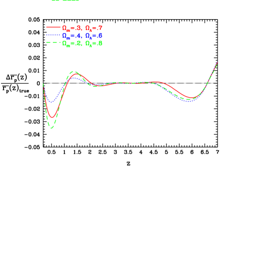
Figure 1: The accuracy with which the scaled distance $\overline{r_{p}}(z)=r_{p}(z)/r_{p}(0.17)$ can be reconstructed using cubic spline interpolation (C.S.) from $\{\overline{r_{p}}(z_{i})\}$ for $N_{bin}=6$ with our choice of binning. Note that $\Delta\overline{r_{p}}(z)=\overline{r_{p}}(z)_{C.S.}-\overline{r_{p}}(z)_{true}$.

Note that for a given set of possible values of $\{\overline{r_{p}}(z_{i})\}$ ($i=1,2,...,6$), the luminosity distance at an arbitrary redshift, $d_{L}(z)$, is given by the accurate interpolation described above. Thus no assumptions about cosmological parameters are made. We calibrate the GRBs for each set of possible values of $\{\overline{r_{p}}(z_{i})\}$ ($i=1,2,...,6$), and compute the likelihood of this set of $\{\overline{r_{p}}(z_{i})\}$ in a Markov Chain Monte Carlo analysis. Hence the distances $\{\overline{r_{p}}(z_{i})\}$ are independent of assumptions about cosmological parameters.

II.3 Other cosmological data

GRB data alone do not constrain dark energy parameters. In order to investigate how well our model-independent distance measurements from GRB represent GRB data, we study them in combination with 307 SNe Ia Kowa08 , Cosmic Microwave Background anisotropy (CMB) data from WMAP five year observations Komatsu et al. (2008), and baryon acoustic oscillation (BAO) scale measurement from the SDSS data Eisenstein et al. (2005).

SN Ia data give the luminosity distance as a function of redshift, $d_{L}(z)=(1+z)\,r(z)$. We use 307 SNe Ia from the “Union” compilation by Ref.Kowa08 , which includes data from Ref.SNdata . Appendix A of Ref.Wang & Mukherjee (2007) describes in detail how we use SN Ia data (flux-averaged to reduce lensing-like systematic effects flux-avg and marginalized over $H_{0}$) in this paper. We applied flux-averaging to the “without systematics” data from the “Union” compilation. The “with systematics” data differ only in having small offsets added to different data sets, which leads to correlations in the data. We expect the increase of uncertainties resulting from flux-averaging to be larger than the effect of the small offsets between different data sets.

We include the CMB data using the method proposed by Ref.Wang & Mukherjee (2007), which showed that the CMB shift parameters

$$R\equiv\sqrt{\Omega_{m}H_{0}^{2}}\,r(z_{*}),\hskip 7.22743ptl_{a}\equiv\pi r(z_{*})/r_{s}(z_{*}),$$ (26)

together with $\Omega_{b}h^{2}$, provide an efficient summary of CMB data as far as dark energy constraints go. We use the covariance matrix of [$R(z_{*}),l_{a}(z_{*}),\Omega_{b}h^{2}]$ from the five year WMAP data (Table 11 of Komatsu et al. (2008)), with $z_{*}$ given by fitting formulae from Hu & Sugiyama (1996) Hu & Sugiyama (1996). CMB data are included in our analysis by adding the following term to the $\chi^{2}$ of a given model with $p_{1}=R(z_{*})$, $p_{2}=l_{a}(z_{*})$, and $p_{3}=\Omega_{b}h^{2}$:

$$\chi^{2}_{CMB}=\Delta p_{i}\left[\mathrm{Cov}_{CMB}^{-1}(p_{i},p_{j})\right]\Delta p_{j},\hskip 14.22636pt\Delta p_{i}=p_{i}-p_{i}^{data},$$ (27)

where $p_{i}^{data}$ are the maximum likelyhood values given in Table 10 of Komatsu et al. (2008).

We also use the SDSS baryon acoustic oscillation (BAO) scale measurement by adding the following term to the $\chi^{2}$ of a model:

$$\chi^{2}_{BAO}=\left(\frac{A-A_{BAO}}{\sigma_{A}}\right)^{2},$$ (28)

where $A$ is defined as

$$A=\left[r^{2}(z_{BAO})\,\frac{cz_{BAO}}{H(z_{BAO})}\right]^{1/3}\,\frac{\left(\Omega_{m}H_{0}^{2}\right)^{1/2}}{cz_{BAO}},$$ (29)

and $A_{BAO}=0.469\,(n_{S}/0.98)^{-0.35}$, $\sigma_{A}=0.017$, and $z_{BAO}=0.35$ (independent of a dark energy model) Eisenstein et al. (2005). We take the scalar spectral index $n_{S}=0.96$ as measured by WMAP five year observations Komatsu et al. (2008).

Finally, in combination with CMB data, we include the Hubble Space Telescope (HST) prior on the Hubble constant of $h=0.72\pm 0.08$ HST_H0 .

III Results

For Gaussian distributed measurements, the likelihood function $L\propto e^{-\chi^{2}/2}$, with

$$\chi^{2}=\chi^{2}_{GRB}+\chi^{2}_{SNe}+\chi^{2}_{CMB}+\chi^{2}_{BAO},$$ (30)

where $\chi^{2}_{GRB}$ is given in Eqs.(III)-(III), $\chi^{2}_{SNe}$ is given in Appendix A of Ref.Wang & Mukherjee (2007), $\chi^{2}_{CMB}$ is given in Eq.(27), and $\chi^{2}_{BAO}$ is given in Eq.(28).

We run a Monte Carlo Markov Chain (MCMC) based on the MCMC engine of Lewis02 (2002) to obtain ${\cal O}$($10^{6}$) samples for each set of results presented in this paper. For the model-independent GRB distance measurements, the parameter set is $\{\overline{r_{p}}(z_{i})\}$ ($i=1,2,...,6$); no assumptions are made about cosmological parameters. For the combined analysis of GRBs (using either the model-independent distance measurements $\{\overline{r_{p}}(z_{i})\}$ ($i=1,2,...,6$), or the 69 GRBs directly) with other cosmological data, the cosmological parameter sets used are: $\Omega_{m}$ for a flat Universe with a cosmological constant; ($\Omega_{m}$, $\Omega_{\Lambda}$) for a cosmological constant; ($\Omega_{m}$, $w_{0}$) for a flat Universe with a constant dark eneagy equation of state; and ($\Omega_{m}$, $h$, $\Omega_{b}h^{2}$, $p_{\mathrm{DE}}$) for a flat Universe with a dark eneagy equation of state linear in the cosmic scale factor, with $p_{\mathrm{DE}}=(w_{0}$, $w_{0.5}$) or ($w_{0}$, $w_{a}$). We assum flat priors for all the parameters, and allow ranges of the parameters wide enough such that further increasing the allowed ranges has no impact on the results. The chains typically have worst e-values (the variance(mean)/mean(variance) of 1/2 chains) much smaller than 0.005, indicating convergence. The chains are subsequently appropriately thinned to ensure independent samples.

Fig.2 shows the distances $\{\overline{r_{p}}(z_{i})\}$ measured from 69 GRBs using the five calibration relations in Eqs.(1)-(5). Table 2 gives the mean and 68% confidence level errors of $\{\overline{r_{p}}(z_{i})\}$. The normalized covariance matrix of $\{\overline{r_{p}}(z_{i})\}$ is given in Table 3. To use our GRB distance measurements to constrain cosmological models, use

$$\chi^{2}_{GRB} = \left[\Delta\overline{r_{p}}(z_{i})\right]\cdot\left(\mathrm{Cov}^{-1}_{GRB}\right)_{ij}\cdot\left[\Delta\overline{r_{p}}(z_{j})\right]$$

$$\Delta\overline{r_{p}}(z_{i}) = \overline{r_{p}}^{\mathrm{data}}(z_{i})-\overline{r_{p}}(z_{i}),$$ (31)

where $\overline{r_{p}}(z)$ is defined by Eq.(25). The covariance matrix is given by

$$\left(\mathrm{Cov}_{GRB}\right)_{ij}=\sigma(\overline{r_{p}}(z_{i}))\sigma(\overline{r_{p}}(z_{j}))\left(\overline{\mathrm{Cov}}_{GRB}\right)_{ij},$$ (32)

where $\overline{\mathrm{Cov}}_{GRB}$ is the normalized covariance matrix from Table 3, and

$$\sigma(\overline{r_{p}}(z_{i})) = \sigma\left(\overline{r_{p}}(z_{i})\right)^{+},\hskip 14.22636pt\mathrm{if}\,\,\overline{r_{p}}(z)\geq\overline{r_{p}}(z)^{\mathrm{data}};$$

$$\sigma(\overline{r_{p}}(z_{i})) = \sigma\left(\overline{r_{p}}(z_{i})\right)^{-},\hskip 14.22636pt\mathrm{if}\,\,\overline{r_{p}}(z)<\overline{r_{p}}(z)^{\mathrm{data}},$$ (33)

where $\sigma\left(\overline{r_{p}}(z_{i})\right)^{+}$ and $\sigma\left(\overline{r_{p}}(z_{i})\right)^{-}$ are the 68% C.L. errors given in Table 2.

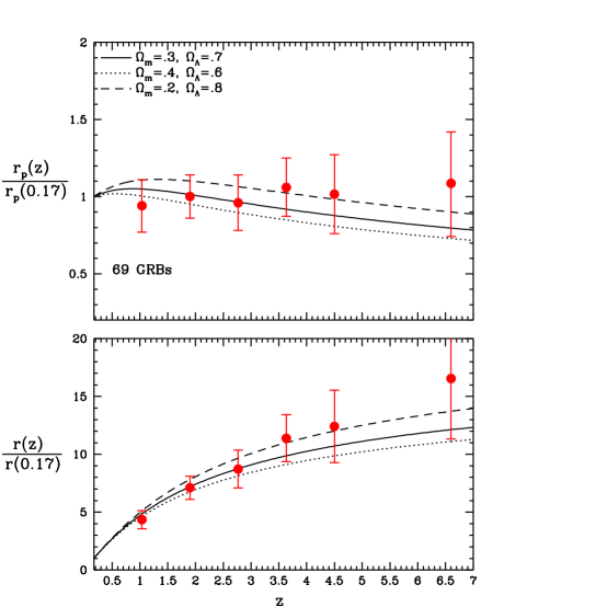
Figure 2: The distances measured from 69 GRBs using the five calibration relations in Eqs.(1)-(5). The error bars indicate the 68% C.L. uncertainties. The top panel shows the scaled distances $r_{p}(z_{i})$ (see Eq.(25)); the bottom panel shows the corresponding comoving distances $r(z_{i})$.

Table 2: Distances measured from 69 GRBs with 68% C.L. upper and lower uncertainties.

	$z$	$\overline{r_{p}}^{data}(z)$	$\sigma\left(\overline{r_{p}}(z)\right)^{+}$	$\sigma\left(\overline{r_{p}}(z)\right)^{-}$
0	0.17	1.0000	–	–
1	1.036	0.9416	0.1688	0.1710
2	1.902	1.0011	0.1395	0.1409
3	2.768	0.9604	0.1801	0.1785
4	3.634	1.0598	0.1907	0.1882
5	4.500	1.0163	0.2555	0.2559
6	6.600	1.0862	0.3339	0.3434

Table 3: Normalized covariance matrix of distances measured from 69 GRBs

	1	2	3	4	5	6
1	1.0000	0.7056	0.7965	0.6928	0.5941	0.5169
2	0.7056	1.0000	0.5653	0.6449	0.4601	0.4376
3	0.7965	0.5653	1.0000	0.5521	0.5526	0.4153
4	0.6928	0.6449	0.5521	1.0000	0.4271	0.4242
5	0.5941	0.4601	0.5526	0.4271	1.0000	0.2999
6	0.5169	0.4376	0.4153	0.4242	0.2999	1.0000

Using the distance measurements from GRBs (see Tables 2 and 3), we find $\Omega_{m}=$0.247 (0.122, 0.372) (mean and 68% C.L. range). Using the 69 GRBs directly, we find $\Omega_{m}=$0.251 (0.135, 0.365). This demonstrates that our model-independent distance measurements from GRBs can be used as a useful summary of the current GRB data.

Fig.3 shows the joint confidence contours for ($\Omega_{m}$, $\Omega_{\Lambda}$), from an analysis of 307 SNe Ia with and without 69 GRBs, assuming a cosmological constant. This shows that the addition of GRB data significantly reduces the uncertainties in ($\Omega_{m}$, $\Omega_{\Lambda}$), and shifts the bestfit parameter values towards a lower matter density Universe. Fig.4 shows the joint confidence contours for ($w_{0}$, $\Omega_{m}$), from an analysis of 307 SNe Ia with and without 69 GRBs, assuming a flat Universe. This shows that SNe Ia alone rules out a cosmological constant at greater than 68% C.L., but the addition of GRB data significantly shifts the bestfit parameter values, and a cosmological constant is consistent with combined SN Ia and GRB data at 68% C.L.

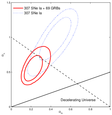
Figure 3: The joint confidence contours for ($\Omega_{m}$, $\Omega_{\Lambda}$), from an analysis of 307 SNe Ia with and without 69 GRBs. A cosmological constant is assumed.

We now consider a dark energy equation of state linear in the cosmic scale factor $a$. Fig.5 shows the joint confidence contours for ($w_{0}$, $w_{0.5}$) and ($w_{0}$, $w_{a}$), from a joint analysis of 307 SNe Ia with CMB data from WMAP5, and SDSS BAO scale measurement, with and without 69 GRBs. HST prior on $H_{0}$ has been imposed and a flat Universe is assumed. Note that $w_{0.5}=w_{X}(z=0.5)$ in the linear parametrization Wang08

$$w_{X}(a) = \left(\frac{a_{c}-a}{a_{c}-1}\right)w_{0}+\left(\frac{a-1}{a_{c}-1}\right)w_{0.5}$$ (34)

$$= \frac{a_{c}w_{0}-w_{0.5}+a(w_{0.5}-w_{0})}{a_{c}-1}$$

with $a_{c}=2/3$ (i.e., $z_{c}=0.5$). Eq.(34) corresponds to a dark energy density function

$$X(z)=\frac{\rho_{X}(z)}{\rho_{X}(0)} = \exp\left\{3\left[1+\left(\frac{a_{c}w_{0}-w_{0.5}}{a_{c}-1}\right)\right]\,\ln(1+z)\right.$$ (35)

$$+\left.3\left(\frac{w_{0.5}-w_{0}}{a_{c}-1}\right)\frac{z}{1+z}\right\}$$

Eq.(34) is related to $w_{X}(z)=w_{0}+(1-a)w_{a}$ Chev01 by setting Wang08

$$w_{a}=\frac{w_{0.5}-w_{0}}{1-a_{c}},\hskip 28.45274pt{\rm or}\hskip 28.45274ptw_{0.5}=w_{0}+(1-a_{c})w_{a}.$$ (36)

Ref.Wang08 showed that ($w_{0}$, $w_{0.5}$) are much less correlated than ($w0$, $w_{a}$), thus are a better set of parameters to use. Fig.5 shows that the addition of GRB data notably shifts the 68% C.L. contours of ($w_{0}$,$w_{0.5}$) and ($w_{0}$, $w_{a}$) to enclose the cosmological constant model ($w_{X}(a)=-1$).

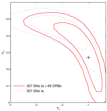
Figure 4: The joint confidence contours for ($w_{0}$, $\Omega_{m}$), from an analysis of 307 SNe Ia with and without 69 GRBs. A flat Universe and dark energy with constant equation of state are assumed.

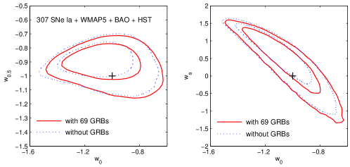
Figure 5: The joint confidence contours for ($w_{0}$, $w_{0.5}$) and ($w_{0}$, $w_{a}$), from a joint analysis of 307 SNe Ia with CMB data from WMAP5, and SDSS BAO scale measurement, with and without 69 GRBs. HST prior on $H_{0}$ has been imposed and a flat Universe is assumed.

IV Summary and Discussion

We have shown that the current GRB data, consisting of 69 GRBs spanning the redshift range from 0.17 to 6.6, can be summarized by a set of distance measurements (see Fig.2). For each set of possible distance values, the GRBs are calibrated. The resultant distance measurements (given in Tables 2 and 3) are independent of cosmology, and can be easily used to combine with other cosmological data sets to constrain dark energy (see Eqs.[III]-[III] and [25]).

The number of bins used in our distance measurement, $n_{bin}=6$, is determined by the current sample of GRBs. Increasing the number of bins by one leads to oscillations in the measured distance values. As more GRB data become available, we can expect to be able to increase the number of bins used to represent GRB data.

We find that GRB data alone give $\Omega_{m}=0.25^{+0.12}_{-0.11}$ for a flat Universe with a cosmological constant. Fig.3 and Fig.4 show that combining GRB data with SN Ia data significantly shifts the bestfit model towards a lower matter density Universe, in agreement with galaxy redshift survey Tegmark06 and CMB data Dunkley08 . Fig.5 shows that assuming a dark energy equation of state linear in cosmic scale factor $a$, including GRB data together with SN Ia, CMB, and BAO data shifts the 68% C.L. contours of the two dark energy parameters to enclose the cosmological constant model.

For a flat Universe with a cosmological constant, our results for GRBs alone differ from that of Ref.Schaefer07 . We find $\Omega_{m}=0.25^{+0.12}_{-0.11}$, while Ref.Schaefer07 found $\Omega_{m}=0.39^{+0.12}_{-0.08}$. The difference likely resulted from the different numerical methods used to calibrate the GRBs. We have fitted straight lines to the calibration relations using errors in both $x$ and $y$ coordinates (see Eq.[8]), while Ref.Schaefer07 used “ordinary least squares without any weighting”. Our results are consistent with the results of Ref.Liang08 , who used SNe Ia to help calibrate the GRBs and found $\Omega_{m}=0.25_{-0.05}^{+0.04}$.

In our quest to solve the mystery of dark energy, GRBs will provide a unique and complementary probe. Our results will make it very convenient to incorporate GRB data in any joint cosmological data analysis in a simple and robust manner.

Acknowledgements I acknowledge the use of getdist from cosmomc in processing the MCMC chains.

References

- (1) Paczynski, B., 1995, PASP, 107, 1167.
- (2) Meszaros, P., Rep. Prog. Phys., 69, 2259 (2006)
- (3) Ghirlanda, G. et al. 2004, ApJ, 613, L13; Dai, Z. G., Liang, E. W., & Xu, D. 2004, ApJ, 612, L101; Firmani, C., Ghisellini, G., Ghirlanda, G., & Avila-Reese, V. 2005, MNRAS, 360, L1; Liang, E. W. & Zhang, B. 2005, ApJ, 633, 603; Firmani, C., Avila-Reese, V., Ghisellini, G., & Ghirlanda, G. 2006, MNRAS, 372, L28; Ghirlanda, G., Ghisellini, G., & Firmani, C. 2006, New J. Phys, 8, 123; Firmani, C., Avila-Reese, V., Ghisellini, G., & Ghirlanda, G. 2007, RMxAA, 43, 203; Kodama, Y. et al. 2008, MNRAS in press (arXiv:0802.3428); Amati, L. et al. 2008, arXiv:0805.0377; Basilakos, S., & Perivolaropoulos, L. 2008, arXiv:0805.0875; Capozziello, S. & Izzo, L. arXiv:0806.1120; Wei, H., & Zhang, S. N. 2008, arXiv:0808.2240; Liang, N., & Zhang, S. N. 2008, arXiv:0808.2655
- (4) Padmanabhan, T, Phys.Rep., 380, 235 (2003); Peebles, P. J. E., & Ratra, B., Rev. Mod. Phys., 75, 55 (2003); Sahni, V., & Starobinsky, A., IJMPD, 15, 2105 (2006) Copeland, E. J., Sami, M., & Tsujikawa, S., IJMPD, 15, 1753 (2006); Ruiz-Lapuente, P., Class. Quantum. Grav., 24, 91 (2007); Ratra, B., & Vogeley, M. S., PASP, 120, 235 (2008)
- (5) Schaefer, B. E. 2004, ApJ, 602, 306.
- (6) Schaefer, B. E., 2007, ApJ, 660, 16
- (7) Liang, N., Xiao, W. K., Liu, Y., Zhang, S. N. 2008, ApJ, in press, arXiv:0802.4262
- (8) Press, W.H., Teukolsky, S.A., Vettering, W.T., & Flannery, B.P. 2007, Numerical Recipes 3rd Edition, Cambridge University Press, Cambridge.
- (9) Kowalski, M., et al., 2008, arXiv:0804.4142
- Komatsu et al. (2008) Komatsu, E., et al., arXiv:0803.0547 [astro-ph]
- Eisenstein et al. (2005) Eisenstein, D., et al., ApJ, 633, 560
- (12) M. Hamuy, et al., AJ, 112, 2398 (1996); Riess, A. G., et al., AJ, 116, 1009 (1998); Riess, A. G., et al., AJ, 117, 707 (1999); Perlmutter, S., et al., ApJ, 517, 565 (1999); Tonry, J. L., et al., ApJ, 594, 1 (2003); Knop, R. A., ApJ, 598, 102 (2003); Krisciunas, K., et al., AJ, 127, 1664 (2004a); Krisciunas, K., et al., AJ, 128, 3034 (2004b); Barris, B. J., ApJ, 602, 571 (2004); Jha, S., et al., AJ, 131, 527 (2006); Astier, P., A&A, 447, 31 (2006); Riess, A. G., et al., ApJ, 659, 98 (2007) Miknaitis, G., et al., ApJ, 666, 674 (2007)
- (13) Wang, Y., ApJ 536, 531 (2000b); Wang, Y., & Mukherjee, P. 2004, ApJ, 606, 654; Wang, Y., JCAP, 03, 005 (2005)
- Wang & Mukherjee (2007) Wang, Y., & Mukherjee, P., PRD, 76, 103533 (2007)
- Hu & Sugiyama (1996) Hu, W., & Sugiyama, N. 1996, ApJ, 471, 542
- (16) Freedman, W. L., et al. 2001, ApJ, 553, 47
- Lewis02 (2002) Lewis, A., & Bridle, S. 2002, PRD, 66, 103511
- (18) Wang, Y., PRD, 77, 123525 (2008)
- (19) Chevallier, M., & Polarski, D. 2001, Int. J. Mod. Phys. D10, 213
- (20) Tegmark, M., et al. 2006, Phys. Rev. D74, 123507
- (21) Dunkley, J., et al. 2008, arXiv:0803.0586