Properties of anisotropic magnetic impurities on surfaces

Abstract

Using numerical renormalization group techniques, we study static and dynamic properties of a family of single-channel Kondo impurity models with axial magnetic anisotropy $DS_{z}^{2}$ terms; such models are appropriate to describe magnetic impurity atoms adsorbed on non-magnetic surfaces, which may exhibit surface Kondo effect. We show that for positive anisotropy $D$ and for any spin $S$, the systems behave at low temperatures as regular Fermi liquids with fully compensated impurity spin. The approach to the stable fixed point depends on the value of the spin $S$ and on the ratio $D/T_{K}^{(0)}$, where $T_{K}^{(0)}$ is the Kondo temperature in the absence of the anisotropy. For $S=1$, the screening occurs in two stages if $D<T_{K}^{(0)}$; the second Kondo temperature is exponentially reduced in this case. More generally, there is an effective spin-$1/2$ Kondo effect for any integer $S$ if $D<T_{K}^{(0)}$ and for any half-integer $S$ if $D>T_{K}^{(0)}$. For negative anisotropy $D$, the system is a non-Fermi liquid with residual anisotropic exchange interaction. However, the presence of transverse magnetic anisotropy $E(S_{x}^{2}-S_{y}^{2})$ restores Fermi-liquid behavior in real systems.

I Introduction

As the sizes of the active components in magnetic devices shrink, the ratio of the surface area over bulk volume steadily increases and the importance of surface and interface effects grows. In the past, the focus has mostly been on the magnetic properties of clean surfaces, thin films, and interfaces in multilayers Wiesendanger et al. (1992); Farle (1998); Heinze et al. (2000); Vaz et al. (2008), but now magnetism of nanostructures is emerging as a new subfield with the aim of exploring and modifying the exchange interaction at the nanometer level. Given that the symmetry in the surface area is always reduced as compared to the bulk, more attention needs to be given to possible additional surface-induced magnetic anisotropy effects Heinze et al. (2000); Gambardella et al. (2002); Rusponi et al. (2003); Kuch (2003); Heinrich et al. (2004); Bode et al. (2007); Hirjibehedin et al. (2007); Ferriani et al. (2008); Vaz et al. (2008). Recently, magnetic anisotropy on surfaces studied at the atomic level has become a new focus of interest with potential applications in ultra-dense magnetic data storage. Using scanning tunneling spectroscopy, the magnetic anisotropy can be measured on the single-atom level by analyzing the splittings of magnetic excitation peaks as a function of the applied magnetic field Heinrich et al. (2004); Hirjibehedin et al. (2007). Magnetic anisotropy constants were found to be very large, often in the $\mathrm{meV}$/atom range Gambardella et al. (2002, 2003); Hirjibehedin et al. (2007).

Single magnetic impurity atoms adsorbed on surfaces or buried in the near-surface regions can be described using quantum impurity models Hewson (1993); Bulla et al. (2008) with anisotropy terms Újsághy et al. (1996); Hirjibehedin et al. (2007). The dominant anisotropy terms are of the form $D({\boldsymbol{S}}\cdot{\boldsymbol{n}})^{2}$, where ${\boldsymbol{n}}$ is a vector along a privileged axis that is commonly chosen to be the $z$-axis Újsághy et al. (1996); Újsághy and Zawadowski (1999). The most important contributions seem to arise from the local spin-orbit coupling, as the reduced symmetry leads to unequal hybridization of the different $d$-orbitals of the impurity atom Szunyogh et al. (2006); Szilva et al. (2008). For an impurity buried in the near-surface region, $D$ depends on the distance from the surface and oscillates in sign Szilva et al. (2008).

Numerical calculations and experiments show that the magnetic anisotropy strongly depends on the microscopic details. Depending on the impurity species and on the substrate, different directions of the privileged axis may be found. Density functional theory calculation predict, for example, that perpendicular anisotropy is common for single adatoms on metallic surfaces Etz et al. (2008).

Spin-excitation spectroscopy using a scanning tunneling microscope (STM) has revealed a rich variety of different classes of behavior. For example, for Fe (spin-$2$) adatom on a thin CuN decoupling layer on a Cu surface, the anisotropy is negative with the $z$-axis in the surface plane, along the direction of nitrogen atoms, while for Mn (spin-$5/2$) on the same surface, the anisotropy is weaker but with an out-of-plane $z$-axis, however $D$ is still negative Hirjibehedin et al. (2007). No anomalies at the Fermi level (surface Kondo effect Li et al. (1998); Madhavan et al. (1998); Ujsaghy et al. (2000); Schiller and Hershfield (2000); Madhavan et al. (2001)) are observed for $D<0$ Hirjibehedin et al. (2007). For Co (spin-$3/2$) on CuN layer, the anisotropy $D$ is positive and signatures of the Kondo effect are observed in tunneling spectra Heinrich . These results strongly motivate a study of the entire family of the Kondo impurity models for various values of spin and for different signs and magnitudes of the magnetic anisotropy. Due to the low symmetry at the surface, it appears sufficient as a first approximation to consider coupling to a single conduction channel (the one with the largest exchange coupling constant); it is unlikely that coupling constants to two orthogonal channels would be equal under these conditions.

Similar impurity models with large anisotropies also appear in the context of single molecular magnets, e.g. Mn₁₂ or Fe₈. It was possible to attach metallic contacts to these molecules allowing for electron transport measurements Heersche et al. (2006); Jo et al. (2006). The molecules exhibit very large spin values ($S=10$ for Mn₁₂) and a negative-$D$ axial anisotropy term $DS_{z}^{2}$, so that ground states with two polarized large-spin states are favored in the absence of quantum spin tunneling due to the transverse anisotropy $E(S_{x}^{2}-S_{y}^{2})$ terms Romeike et al. (2006a, b); Roosen et al. (2008); Bogani and Wernsdorfer (2008).

Since the ultimate miniaturization limit appears to be storing information in the spin states of single magnetic atoms, it is important to study decoherence by possible magnetic screening effects through nearby conduction electrons (Kondo effect), since the goal is to have long-lived large-spin magnetic impurity states. The appropriate model is thus the impurity Kondo model with additional anisotropy terms that we introduce in Sec. II. In Sec. III we relate these models by means of scaling equations to the Kondo models with XXZ anisotropic exchange coupling to the conduction band. Numerical renormalization group results are presented in Sec. IV where we compare calculations for $S=1$, $S=3/2$ and $S=2$. $S=3/2$ is a typical representative for all half-integer-spin models, $S=2$ a typical representative for all integer-spin models, while $S=1$ is a special case with some additional features when compared to higher integer spins. We present results both for static properties (magnetic susceptibility, impurity entropy) and for dynamic properties (spectral functions, dynamic magnetic susceptibility). This section also contains a discussion of the various fixed points, focusing on the non-Fermi-liquid behavior in the $D<0$ models.

II Model

A general approach to study the anisotropy effects of adsorbed impurity atoms would start with a multi-orbital Anderson model for the $d$-orbitals with a suitable hybridization function for the coupling with the substrate and with electron-electron repulsion and Hund coupling parameters extracted, for example, from density functional theory calculations. The next step would then consist of obtaining an effective Kondo-like model using a Schrieffer-Wolff transformation. We aim, however, to explore only the effects due to local magnetic anisotropy effects. We thus study a very simplified Kondo impurity model defined by the following Hamiltonian:

$$\begin{split}H&=H_{\mathrm{band}}+H_{\mathrm{K}}+H_{\mathrm{aniso}},\\ H_{\mathrm{band}}&=\sum_{{\boldsymbol{k}}\sigma}\epsilon_{{\boldsymbol{k}}}c^{\dagger}_{{\boldsymbol{k}}\sigma}c_{{\boldsymbol{k}}\sigma},\\ H_{\mathrm{K}}&=J{\boldsymbol{s}}\cdot{\boldsymbol{S}}.\\ \end{split}$$ (1)

Here operators $c_{{\boldsymbol{k}}\sigma}$ describe the conduction band electrons with momentum ${\boldsymbol{k}}$ and spin $\sigma\in\{\uparrow,\downarrow\}$. In numerical calculations, we will for simplicity assume a flat band $\epsilon_{{\boldsymbol{k}}}=Wk$, where the dimensionless momentum (energy) $k$ ranges from $-1$ to $1$ and $W$ is the half-bandwidth; the density of states is thus constant, $\rho=1/(2W)$. Furthermore, the effective exchange constant $J$ is defined as

$$J=\frac{1}{N^{2}}\sum_{{\boldsymbol{k}}{\boldsymbol{k}}^{\prime}}J_{{\boldsymbol{k}},{\boldsymbol{k}}^{\prime}},$$ (2)

where $J_{{\boldsymbol{k}},{\boldsymbol{k}}^{\prime}}$ describe exchange scattering of the conduction band electrons on the impurity, and the spin-density of the conduction band electrons ${\boldsymbol{s}}$ is defined as

$${\boldsymbol{s}}=\frac{1}{N}\sum_{{\boldsymbol{k}}{\boldsymbol{k}}^{\prime}\alpha\alpha^{\prime}}\frac{J_{{\boldsymbol{k}},{\boldsymbol{k}}^{\prime}}}{J}c^{\dagger}_{{\boldsymbol{k}}\alpha}\left(\frac{1}{2}\boldsymbol{\sigma}_{\alpha\alpha^{\prime}}\right)c_{{\boldsymbol{k}}^{\prime}\alpha^{\prime}}.$$ (3)

If $J_{{\boldsymbol{k}},{\boldsymbol{k}}^{\prime}}\equiv J$ is constant, then ${\boldsymbol{s}}$ can be interpreted as the spin-density of conduction band electrons at the position of the impurity. For an impurity adsorbed on a surface, this clearly cannot be a good approximation as the exchange interaction $J_{{\boldsymbol{k}},{\boldsymbol{k}}^{\prime}}$ is inevitably anisotropic in the reciprocal space; nevertheless, since we focus mostly on the role of the local magnetic anisotropy terms, we will not pursue this issue in this work. We furthermore assumed that the exchange interaction is isotropic in the spin space.

In the anisotropy term of the Hamiltonian,

$$H_{\mathrm{aniso}}=DS_{z}^{2}+E\left(S_{x}^{2}-S_{y}^{2}\right),$$ (4)

the first term is the axial magnetic anisotropy, while the second is named the transverse magnetic anisotropy. The axis $z$ is by convention chosen such that $|D|$ is maximized, while axes $xy$ are oriented so that $E>0$. If the axial anisotropy term is negative, $D<0$, we call the $z$ axis an easy axis; if, however, $D>0$ the anisotropy is said to be hard-axis (or planar). Axial anisotropy term $D$ leads to the splitting of magnetic levels, Fig. 1. In the case of easy-axis anisotropy, $D<0$, the moment tends to be maximal in size with two degenerate states pointing in the opposite directions, i.e. $S_{z}=\pm S$. Since the conduction band electrons can only change the impurity spin by one unit during a spin-flip scattering event, the exchange scattering rate is expected to be strongly reduced for large enough $|D|$. In the case of hard-axis anisotropy, $D>0$, the single level $S_{z}=0$ is favored for integer $S$ and the doublet $S_{z}=\pm 1/2$ for half-integer $S$; in both cases, the impurity moment will be compensated at low temperatures, since the doublet can be screened via the conventional spin-$1/2$ Kondo screening. It should be noted that $E(S_{x}^{2}-S_{y}^{2})=E/2\left[(S^{+})^{2}+(S^{-})^{2}\right]$ term, i.e. the transverse anisotropy, mixes levels with different values of $S_{z}$. This term, even when $E$ is small, plays an essential role in the easy-axis case Romeike et al. (2006a); in the hard-axis case, however, it only leads to a small correction.

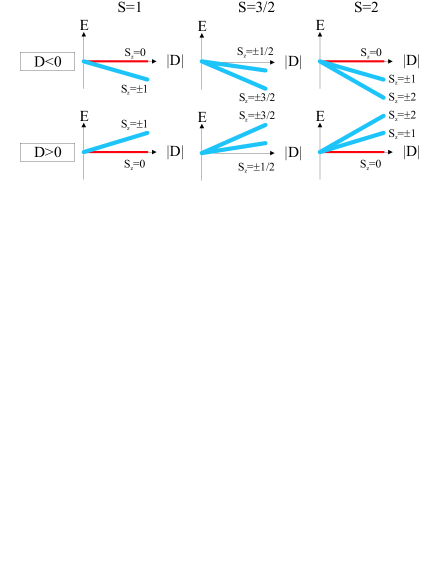
Figure 1: (Color online) Energy level diagrams for the anisotropic magnetic impurities with spin $1$, $3/2$ and $2$ as a function of the absolute value of the anisotropy, $|D|$. Wide (blue) lines represent pairs of states, narrow (red) lines represent non-degenerate states.

The isotropic Kondo model (i.e. the $D=E=0$ limit) has been intensively studied by a variety of techniques, such as numerical renormalization group Cragg and Lloyd (1979); Cragg et al. (1980); Mehta et al. (2005); Koller et al. (2005), Bethe Ansatz Furuya and Lowenstein (1982); Andrei et al. (1983); Andrei and Destri (1984); Andrei (1994); Sacramento and Schlottmann (1989, 1991), and other methods Nozières and Blandin (1980); Coleman and Pepin (2003); Bortz and Klümper (2004). These studies have uncovered the physics of underscreening: a single conduction channel can screen at most $1/2$ unit of spin, so that at low temperatures the impurity remains magnetic with a residual spin of $S-1/2$ Mattis (1967). It was found that for $S\geq 1$ the approach to the stable Fermi-liquid fixed point is slow (logarithmic); this behavior was characterized as that of a singular Fermi liquid Mehta et al. (2005); Koller et al. (2005).

The anisotropic Kondo model with $D\neq 0$ (and with additional anisotropy in the exchange coupling) was studied by the Bethe-Ansatz technique Schlottmann (2000, 2001). It was shown that anisotropy can induce a quantum critical point (i.e. non-Fermi-liquid behavior). The applicability of the Bethe-Ansatz approach is, however, limited to a set of models with restrained parameters thus a direct comparison with the model considered in this work is not possible. Nevertheless, there is qualitative agreement in that we also find a non-Fermi-liquid state for $D<0$.

The anisotropic Kondo model was also previously studied by the numerical renormalization group technique in Refs. Romeike et al., 2006a and Romeike et al., 2006b with the focus on high values of spin $S$ and easy-axis anisotropy as appropriate for molecular magnets (we note that the definition of $D$ in the cited works differs in sign from ours). Where comparisons can be made, our results agree with theirs.

Finally, we mention that related models and physical effects are also studied in the context of transport spectroscopy of quantum dots and impurity clusters. The high conductance in the case of underscreening in spin-$1$ quantum dots and the two-stage Kondo screening were discussed in Refs. Posazhennikova and Coleman, 2005 and Posazhennikova et al., 2007. Furthermore, the two-stage Kondo screening is also found in the case of a single conduction channel in multiple-quantum-dot structures, in particular in the case of side-coupled quantum dots Vojta et al. (2002a); Cornaglia and Grempel (2005); Žitko and Bonča (2006); Chung et al. (2008). High-spin states can be obtained in systems of multiple impurities if the conduction-band-mediated exchange interaction is ferromagnetic Žitko and Bonča (2006, 2007), which may occur for small inter-impurity separations. Two-stage Kondo screening and the closely related “singlet-triplet” Kondo effect Izumida et al. (2001); Pustilnik and Glazman (2001a, b); Sakai and Izumida (2003); Pustilnik et al. (2003); Hofstetter and Zaránd (2004) have both been intensively studied experimentally Schmid et al. (2000); Sasaki et al. (2000); van der Wiel et al. (2002); Kogan et al. (2003); Fuhrer et al. (2003); Granger et al. (2005).

III Scaling analysis

There is a close relation Konik et al. (2002); Schiller and De Leo (2008) between the Kondo model with the $DS_{z}^{2}$ magnetic anisotropy term and the Kondo model with the XXZ anisotropic exchange constants $J_{z}$ and $J_{\perp}$ Anderson (1970); Tsvelick and Wiegmann (1983); Costi and Kieffer (1996); Costi (1998); Schiller and De Leo (2008) defined by the Hamiltonian

$$H_{\mathrm{K}}=J_{z}s_{z}S_{z}+J_{\perp}\left(s_{x}S_{x}+s_{y}S_{y}\right).$$ (5)

To be specific, we consider here the $S=1$ anisotropic Kondo model with both types of the anisotropy (XXZ exchange and the $DS_{z}^{2}$ term, but $E=0$). Taking into account that the energy of the $S_{z}=\pm 1$ intermediate states is higher by $D$ as compared with the energy of the $S_{z}=0$ state, the following scaling equations are obtained Anderson (1970); Konik et al. (2002); Schiller and De Leo (2008)

$$\frac{\mathrm{d}j_{z}}{\mathrm{d}l} =\frac{1}{1-d}j_{\perp}^{2},$$ (6)

$$\frac{\mathrm{d}j_{\perp}}{\mathrm{d}l} =\frac{1}{2}\left(1+\frac{1}{1+d}\right)j_{\perp}j_{z},$$ (7)

$$\frac{\mathrm{d}d}{\mathrm{d}l} =d-\ln 2\left(j_{z}^{2}-j_{\perp}^{2}\right).$$ (8)

Here the scaling parameter is $l=-\ln W$; it runs from 0 to positive infinity as the energy scale is reduced. Note that here we denote the half-bandwidth by $W$ (this departs from the NRG convention of denoting it by $D$). We have introduced dimensionless running coupling constants by absorbing the density of states $\rho$: $j_{\perp}=\rho J_{\perp}$, $j_{z}=\rho J_{z}$, while $d$ is measured in the units of $W$: $d=D/W$. These scaling equations differ from those in Ref. Schiller and De Leo, 2008 only by the $d$-dependent factors in Eqs. (6) and (7), which arise due to the energy shift by $D$ in the $S_{z}=\pm 1$ states.

From Eq. (8) it follows that $d$ will rapidly grow in absolute value Schiller and De Leo (2008), since the $d$ term on the right hand side is first order, while the $j_{z}^{2}$ and $j_{\perp}^{2}$ terms are second order, hence smaller. The importance of the axial anisotropy is thus always reinforced at lower energy scales. Furthermore, starting from initially equal bare coupling constants, $j_{z}=j_{\perp}$, a non-zero $d$ induces XXZ exchange anisotropy by unequal renormalization of $j_{z}$ and $j_{\perp}$, as seen from Eqs. (6) and (7). At low energy scales, the physical properties are qualitatively the same irrespective of the origin of the anisotropy. From Eq. (8) we may also anticipate that the $D>0$ case corresponds to a $J_{\perp}>J_{z}$ exchange anisotropic Kondo model, while the $D<0$ case to a $J_{\perp}<J_{z}$ model Schiller and De Leo (2008).

IV Numerical results

Calculations were performed using the numerical renormalization group technique Wilson (1975); Cragg and Lloyd (1979); Cragg et al. (1980); Krishna-murthy et al. (1980); Hewson (1993); Bulla et al. (2008) which consists of a logarithmic discretization of the continuum of states of the conduction band electrons, followed by mapping to a one-dimensional chain Hamiltonian with exponentially decreasing hopping constants. This Hamiltonian is then diagonalized iteratively by taking into account one new lattice site at each iteration. We have used discretization parameter $\Lambda=2.5$ ($\Lambda=2$ for spectral function calculations) and truncation with the energy cutoff at $E_{\mathrm{cutoff}}=10\omega_{N}$, where $\omega_{N}$ is the characteristic energy scale at the $N$-th iteration step. As a further precaution, truncation is always performed in a “gap” of width at least $0.01\omega_{N}$, so as not to introduce systematic errors. To prevent spurious polarization of the residual impurity spin in the $D<0$ case due to floating-point round-off errors, it is helpful to symmetrize the energies of states which should be exactly degenerate (i.e. the $\pm S_{z}$ pairs). In all calculations, we have taken explicitly into account the conservation of charge $Q$; in calculations with only the $DS_{z}^{2}$ anisotropy term ($E=0$), a further conserved quantum number is $S_{z}$.

In all calculations we set $\rho J=0.1$, therefore the Kondo temperature in the isotropic case, $T_{K}^{(0)}$, is the same for all values of spin $S$ Andrei et al. (1983); Bortz and Klümper (2004); Kaihe and Zhao (2005); Žitko and Bonča (2006) and given by Wilson (1975); Krishna-murthy et al. (1980):

$$T_{K}^{(0)}\approx W\sqrt{\rho J}\exp\left(-\frac{1}{\rho J}\right)=1.4\times 10^{-5}W.$$ (9)

Extracting $T_{K}^{(0)}$ directly from the NRG results we obtain a more accurate value of $T_{K}^{(0)}=1.16\times 10^{-5}W$. (We use Wilson’s definition of the Kondo temperature Wilson (1975); Andrei and Lowenstein (1981); Andrei et al. (1983).)

IV.1 Static properties

We first consider the static (thermodynamic) properties, in particular the impurity contribution to the magnetic susceptibility, $\chi_{\mathrm{imp}}$, and the impurity contribution to the entropy, $S_{\mathrm{imp}}$. The first quantity, when multiplied by the temperature, is a measure of the effective magnetic moment at a given temperature scale, while the second provides information about the effective impurity degrees of freedom.

In Fig. 2 we plot the thermodynamic properties of the anisotropic Kondo model with the axial $DS_{z}^{2}$ term ($E=0$) for three different values of the impurity spin $S$ and for a range of the anisotropy strength. As long as the temperature is larger than the anisotropy $D$, the curves follow closely the results for the isotropic case (black curves). At lower temperatures, the behavior of the system strongly depends on the sign of $D$. For negative $D$ (easy-axis case), the impurity spin remains partially unscreened at low temperatures; for small $|D|$, the effective moment is slightly above the isotropic strong-coupling fixed-point value with spin $S-1/2$ [i.e. $\mu=(S^{2}-1/4)/3$] and it saturates with increasing $|D|$ at the value of $\mu=S^{2}$. The low-temperature impurity entropy is $\ln 2$ for all negative $D$. This suggests that the impurity behaves as a residual two-level system with states $|+\rangle$ and $|-\rangle$, which in the large-$|D|$ limit become equal to the $|S_{z}=+S\rangle$ and $|S_{z}=-S\rangle$ states. The scattering of the low-energy electrons on this residual impurity states is discussed in App. A. For spin $S>1$, the effective moment always increases as the temperature $T$ is decreased below $|D|$, which reflects the progressive freezing out of the magnetic levels other than the maximally aligned $S_{z}=\pm S$ states. For spin $1$, this is still the case for large enough $|D|$, but for lower $|D|$ the temperature dependence becomes monotonic. The boundary between the two different behaviors can be approximately located at $|D|\sim T_{K}^{(0)}$. The reason appears to be that for $|D|<T_{K}^{(0)}$, the $S=1$ Kondo effect had already significantly screened the impurity spin yielding a residual spin $1/2$ by the time the anisotropy begins to be felt; the only effect of the anisotropy is then to prevent the screening process from completing, which gives a residual spin value slightly above $1/2$.

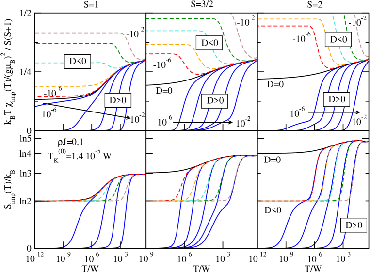
Figure 2: (Color online) Thermodynamic properties of the anisotropic Kondo model. We plot the impurity contribution to the magnetic susceptibility, $\chi_{\mathrm{imp}}$, and the impurity contribution to the entropy, $S_{\mathrm{imp}}$. Full (blue) lines correspond to positive anisotropy, $D>0$, dashed (red) lines correspond to negative anisotropy, $D<0$, while black line is the isotropic case, $D=0$. The arrow indicate in which direction the anisotropy is increasing. Note that the vertical axis in the upper panels is additionally rescaled as $1/S(S+1)$.

For positive $D$ (hard-axis case), the impurity is non-magnetic at low temperatures for any value of the impurity spin $S$. Unlike in the easy-axis case, we see a larger variety of possible behaviors in the approach to the fixed point depending on the spin and on the anisotropy strength. We discuss $S=3/2$ and $S=2$ first; these are characteristic representatives for all half-integer and integer spin cases.

For half-integer spin and small $D<T_{K}^{(0)}$, the curves just follow the results for the isotropic case until $T\sim D$, when spin states other than the $S_{z}=0$ state of the residual (integer!) $S-1/2$ impurity spin freeze out and the system approaches the non-magnetic ground state exponentially fast. For sufficiently large $D>T_{K}^{(0)}$, the high $|S_{z}|$ states of the original impurity spin freeze out exponentially fast at $T\sim D$, this time yielding a $S_{z}=\pm 1/2$ doublet which then undergoes spin-$1/2$ Kondo screening. It must be stressed, however, that after the high-$|S_{z}|$ states are frozen out, the effective model in the restrained $S_{z}=\pm 1/2$ subspace does not correspond to an isotropic spin-$1/2$ model, but rather to an exchange anisotropic spin-$1/2$ model with

$$J_{\perp}\approx 2J,\quad J_{z}\approx J.$$ (10)

The mapping on an anisotropic Kondo model stems from the spin-$3/2$ operators which are given in the matrix notation as

$$\begin{split}S_{x}&=\begin{pmatrix}0&\frac{\sqrt{3}}{2}&0&0\\ \frac{\sqrt{3}}{2}&0&1&0\\ 0&1&0&\frac{\sqrt{3}}{2}\\ 0&0&\frac{\sqrt{3}}{2}&0\end{pmatrix},\\ S_{z}&=\begin{pmatrix}\frac{3}{2}&0&0&0\\ 0&\frac{1}{2}&0&0\\ 0&0&-\frac{1}{2}&0\\ 0&0&0&-\frac{3}{2}\\ \end{pmatrix}.\end{split}$$ (11)

In the $S_{z}=\pm 1/2$ subspace, $S_{z}$ yields $\frac{1}{2}\sigma_{z}$, while $S_{x,y}$ yield $2\times\frac{1}{2}\sigma_{x,y}$, i.e. twice the spin-$1/2$ operators in the transverse directions. The Kondo temperature is thus given by the expression for the XXZ anisotropic Kondo model:

$$\begin{split}T_{K}&\approx W\exp\left(-\frac{\alpha}{\rho J_{z}}\right),\\ \alpha&=\frac{\arctan\gamma}{\gamma},\\ \gamma&=\sqrt{\left(\frac{J_{\perp}}{J_{z}}\right)^{2}-1},\quad\text{for}\,J_{\perp}\geq J_{z},\end{split}$$ (12)

which can be derived from the scaling equations to second order Romeike et al. (2006a). For reference we also note that the expression for $J_{\perp}<J_{z}$ can be obtained by analytic continuation, giving

$$\begin{split}T_{K}&\approx W\exp\left(-\frac{\alpha}{\rho J_{z}}\right),\\ \alpha&=\frac{\mathrm{arctanh}\gamma}{\gamma},\\ \gamma&=\sqrt{1-\left(\frac{J_{\perp}}{J_{z}}\right)^{2}},\quad\text{for}\,J_{\perp}\leq J_{z}.\end{split}$$ (13)

These expressions somewhat overestimate the true Kondo temperature since they do not include the $\sqrt{\rho J_{z}}$ factors; numerically calculated Kondo temperatures are shown in Fig. 3.

The value of the Kondo temperature of the effective spin-$1/2$ screening process depends on $D$ and it can exceed $T_{K}^{(0)}$ since $\alpha<1$ in the transverse dominated $J_{\perp}/J_{z}>0$ case; in the infinite-$D$ limit, $T_{K}(S=1/2)$ goes to

$$T_{K}(S=1/2)\approx 9\times 10^{-4}W.$$ (14)

This result fully agrees with $T_{K}$ in the exchange-anisotropic Kondo model, Fig. 3. For finite $D$, the effective ratio $J_{\perp}/J_{z}$ may be different from 2, since there is a temperature range where the $S_{z}=\pm 3/2$ levels still affect the renormalization of the exchange interaction before they completely freeze out. The intrinsic anisotropy of the effective spin-$1/2$ Kondo model also plays a role in the splitting (shifting) of the Kondo resonance in a magnetic field: for strong magnetic field $B_{z}$ in the $z$-direction, we expect a shift of $\sim g\mu_{B}B_{z}$, and a shift approximately twice as large for fields in the transverse directions Heinrich . Finally, we note that for larger spin values we have $J_{\perp}=3J$ (spin $5/2$), $J_{\perp}=4J$ (spin $7/2$), and in general

$$J_{\perp}=(S+1/2)J.$$ (15)

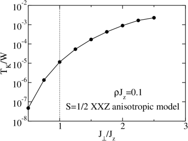
Figure 3: The Kondo temperature of the XXZ anisotropic $S=1/2$ Kondo model as a function of the $J_{\perp}/J_{z}$ ratio.

For integer $S\geq 2$, the situation is the opposite. Now the regime of the exponential approach to the $S_{z}=0$ ground state corresponds to $D>T_{K}^{(0)}$. For $D<T_{K}^{(0)}$, on the other hand, the low-temperature behavior is again that of the spin-$1/2$ Kondo model. This is made possible by the combined effect of the spin-$S$ Kondo screening at higher temperatures giving rise to the $S-1/2$ (i.e. half-integer) residual impurity spin, and of the axial anisotropy which leads to freezing out of the high-spin $S_{z}=\pm(S-1/2),{\ldots},\pm 3/2$ levels of this residual object to finally give rise to a residual spin-$1/2$ object. This residual spin-$1/2$ then finally undergoes a spin-$1/2$ Kondo screening. At first sight it might even seem surprising that the residual spin is compensated at all, given that in the isotropic high-spin Kondo model the residual exchange interaction is ferromagnetic, yet for $D>0$ the induced exchange anisotropy (see Sec. III) is of the type which leads to complete screening of the impurity spin Konik et al. (2002). Since the residual $(S-1/2)$ spin is an extended object, there is no simple mapping on the effective spin-$1/2$ Kondo model and it appears difficult to estimate the effective exchange constants $J_{\perp}$ and $J_{z}$ even in the $D\to 0$ limit. The effective bandwidth on the other hand is clearly given by $W_{\mathrm{eff}}=\alpha D$, where $\alpha$ is some constant of order 1. The Kondo temperature is thus given by $T_{K}(S=1/2)\approx Df(D)$, where $f(D)$ turns out to be a power-law function with non-integer exponent, $f(D)\sim D^{1.3}$ for $S=2$ and $f(D)\sim D^{0.7}$ for $S=3$, see Fig. 4. For large spin the Kondo temperature is simply proportional to $D$.

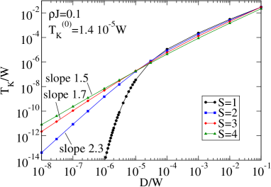
Figure 4: (Color online) The cross-over temperature (indentified with the spin-$1/2$ Kondo temperature $T_{K}$ for $D<T_{K}^{(0)}$) in integer-spin anisotropic Kondo models for the hard-axis case.

We would like to emphasize the important fact that the original impurity spin $S$ and the residual spin $S-1/2$ after the Kondo screening belong to different classes (one is integer, the other half-integer). For this reason we always find different behavior depending on which of the $D$ and $T_{K}^{(0)}$ is smaller. Furthermore, this explains similarities between integer $S$ for $D<T_{K}^{(0)}$ and half-integer $S$ for $D>T_{K}^{(0)}$.

Finally we consider the special case of integer spin 1. For large $D>T_{K}^{(0)}$, the behavior is the same as for other integer spins. For small $D<T_{K}^{(0)}$, the approach to the strong-coupling fixed point is of the spin-$1/2$ Kondo model type. However, we find that the second Kondo temperature $T_{K}^{(2)}$ depends exponentially on the $D/T_{K}^{(0)}$ ratio, see Fig. 4, a situation strongly reminiscent of the two-stage Kondo screening Jayaprakash et al. (1981) in the side-coupled impurity systems Vojta et al. (2002a); Cornaglia and Grempel (2005); Žitko and Bonča (2006); Peters and Pruschke (2006); Chung et al. (2008). At $T_{K}^{(0)}$ the spin is screened from $S=1$ to $S=1/2$ by the spin-$1$ Kondo effect, then at $T_{K}^{(2)}$ from $S=1/2$ to $S=0$ by the spin-$1/2$ Kondo effect. It is possible to fit the results with

$$T_{K}^{(2)}=\alpha T_{K}^{(0)}e^{-\gamma\frac{T_{K}^{(0)}}{J_{\mathrm{eff}}}}$$ (16)

where

$$J_{\mathrm{eff}}=D+cT_{K}^{(0)}$$ (17)

with coefficients $\alpha=0.052$, $\gamma=2.531$, $c=0.0661$. This fit is only of phenomenological value: the situation here is different from the one in the side-coupled impurity case, where it is possible to interpret the results in terms of screening of the second impurity by the quasiparticles resulting from the first stage of the Kondo screening and where $J_{\mathrm{eff}}$ corresponds to real exchange coupling.

In Fig. 5 we plot the thermodynamic quantities for the related $S=1$ Kondo model with XXZ exchange anisotropy Schiller and De Leo (2008). As expected, we find that $J_{\perp}<J_{z}$ models behave similarly to $D<0$, and $J_{\perp}>J_{z}$ similarly to $D>0$. In the presence of both symmetries, the two anisotropies may either enhance each other or compete.

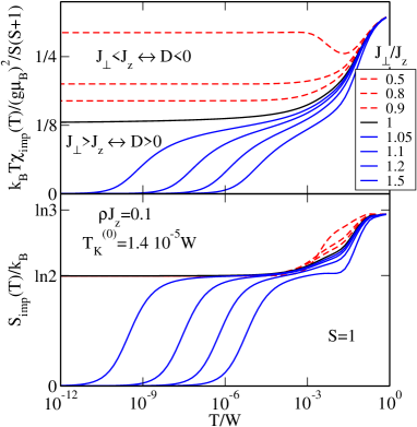
Figure 5: (Color online) Thermodynamic properties of the $S=1$ Kondo model with XXZ exchange anisotropy.

In Fig. 6 we plot the impurity contribution to the entropy for the fully anisotropic problem with the $DS_{z}^{2}$ and $E(S_{x}^{2}-S_{y}^{2})$ terms (impurity contribution to the magnetic susceptibility cannot be easily computed since $S_{z}$ is no longer a good quantum number). We consider both the case when $E$ is large [subfigure a) with $E=0.2|D|$; such ratio is found, for example, for integer spin-$2$ Fe impurities on CuN/Cu surfaces where $D=-1.5\,\mathrm{meV}$ and $E=0.3\,\mathrm{meV}$, and for half-integer spin-$5/2$ Mn impurities on the same surface Hirjibehedin et al. (2007)] and for the case where $E$ is much lower than $|D|$ [subfigure b) with $E=0.01|D|$; no such magnetic adatom/surface system had been identified so far in the negative-$D$ systems, but $E$ appears to be much smaller than $D$ in the positive-$D$ Co on CuN/Cu system].

The ground state for $E\neq 0$ is non-degenerate for all parameters. For $D>0$, the $S_{x}^{2}-S_{y}^{2}$ operator is an irrelevant perturbation and the thermodynamic behavior of the system is hardly affected. For $D<0$, however, the perturbation is relevant and drives the system to a different, non-magnetic ground state for all $S$. For $S=1$, the degeneracy is lifted on the scale of $E$ if $E>T_{K}^{(0)}$; for $E<T_{K}^{(0)}$ there appears to be Kondo-like screening of the residual spin-$1/2$ with exponential reduction of the second Kondo temperature, similar to what happens in the $D>0$ case. Thus the $E$-term can induce two-stage Kondo behavior even in the $D<0$ case. For half-spin $S=3/2$, the degeneracy is again lifted on the scale of $E$ if $E<T_{K}^{(0)}$. If $E>T_{K}^{(0)}$, previously known Kondo effect with pseudo-spin $1/2$ occurs Romeike et al. (2006a); the Kondo temperature depends on parameters in a non-trivial way. For integer spin $S=2$, we find degeneracy lifting on the scale of $E$ if $E>T_{K}^{(0)}$, and a pseudo-spin $1/2$ Kondo effect if $E<T_{K}^{(0)}$. The effective bandwidth is now given by $W_{\mathrm{eff}}=\alpha E$, where $\alpha$ is some constant of order 1, so the Kondo temperature is given by $T_{K}\approx Ef(D,E)$ where $f(D,E)$ has power-law behavior as a function of $D$ with a $D/E$ (and spin $S$) dependent exponent, see Fig. 7.

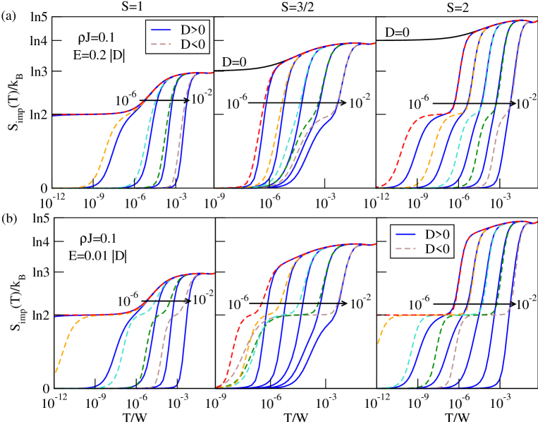
Figure 6: (Color online) Impurity contribution to the entropy of the anisotropic Kondo model with $DS_{z}^{2}+E(S_{x}^{2}-S_{y}^{2})$ terms with constant ratio (a) $E/|D|=0.2$ and (b) $E/|D|=0.01$. We plot $D=10^{-6},10^{-5},{\ldots},10^{-2}$; the arrow indicate in which direction the anisotropy is increasing.

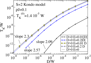
Figure 7: (Color online) The cross-over temperature (indentified with the spin-$1/2$ Kondo temperature $T_{K}$ for $D<T_{K}^{(0)}$) in the $S=2$ anisotropic Kondo model with transverse anisotropy.

We conclude that the easy-axis systems with transverse anisotropy behave rather similarly to hard-axis systems; in the conditions for the emergence of the pseudo-spin $S=1/2$ Kondo effect the quantity $E$ takes the place of $D$.

IV.2 Properties of the $D<0$ systems

For any $S\geq 1$ and $D<0$, $E=0$, the ground state is twofold degenerate. The fixed-point spectra depend on the value of $D$, thus the $S_{z}^{2}$ term is a marginal operator. At low temperatures, these systems have a Curie-like magnetic response with fractional spin

$$\chi_{\mathrm{imp}}(T\to 0)=(g\mu_{B})^{2}\frac{\mathcal{C}(D)}{k_{B}T}.$$ (18)

This is reminiscent of the fractional-spin non-Fermi-liquid fixed points in the pseudo-gap Kondo model with $\rho(\omega)\sim|\omega|^{r}$ density of states for spin 1 and $r>0$ Gonzalez-Buxton and Ingersent (1998); Florens and Vojta (2005); Withoff and Fradkin (1990); Chen and Jayaprakash (1995) and in the related power-law Kondo model in the case of ferromagnetic coupling and $r<0$ Vojta and Bulla (2002). There are nevertheless some notable differences. The fixed points in the pseudo-gap Kondo model are found to be unstable with respect to the particle-hole symmetry breaking. The fixed points we find are, however, stable with respect to particle-hole symmetry breaking: both anisotropy, $S_{z}^{2}$, and potential scattering, $n_{f_{0}}$, are marginal operators. Furthermore, the fixed point in the anisotropic Kondo model has entropy $\ln 2$ (i.e. impurity behaves as a two-level system), while the fixed point in the pseudo-gap Kondo model has entropy $(1+2r)\ln 2$ Gonzalez-Buxton and Ingersent (1998); Florens and Vojta (2005).

In Fig. 8 we plot the Curie constant as a function of the $D/T_{K}^{(0)}$ ratio. The transition from the isotropic limit

$$\mathcal{C}=(S-1/2)(S+1/2)/3=(S^{2}-1/4)/3,$$ (19)

to the saturated easy-axis anisotropic behavior,

$$\mathcal{C}=S^{2},$$ (20)

is approximately logarithmic, i.e. very slow. This reflects the underlying underscreened Kondo effect and the partial screening of the impurity moment which also feature similarly slow logarithmic dependence of the magnetic susceptibility on temperature and magnetic field.

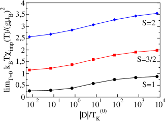
Figure 8: (Color online) Curie constant as a function of the $|D|/T_{K}^{(0)}$ ratio for $S=1,3/2,2$ Kondo models with easy-axis anisotropy, $D<0$.

In Fig. 9 we plot the energy levels of the spin-1 negative-$D$ model as a function of the anisotropy $D$. For small $|D|$, the levels approach the free electron spectrum with $\pi/2$ phase shift (which is due to the Kondo effect) with additional two-fold degeneracy of all levels due to the decoupled spin-$1/2$ residual impurity spin. For large $|D|$, the levels tend towards a spectrum with states clustered near the energies of the free electron spectrum with zero phase shift (no Kondo effect) with additional splitting due to residual anisotropic exchange coupling that will be studied in App. A. For intermediate $|D|$, the spectrum is more complex. It can be characterized as free electron spectrum with some intermediate phase shift with additional splitting due to residual exchange interaction; as $|D|$ is swept from $0$ to $+\infty$, the (spin-dependent) phase shift is reduced from $\pi/2$ to 0, while the nature of the residual impurity spin changes from isotropic spin-$1/2$ doublet to the anisotropic $S_{z}=\pm 1$ magnetic doublet, and the residual exchange constants increase from 0 to some finite value of the order of the bare exchange coupling $J$, see also App. A.

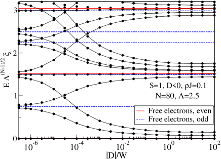
Figure 9: (Color online) Energy levels at iteration $N=80$ ($T\sim 10^{-16}W$) as a function of the anisotropy $D$ in the spin-1 Kondo model with easy-axis anisotropy, $D<0$.

IV.3 Dynamic properties

To characterize dynamic properties of the anisotropic models, we calculate the T-matrix and the dynamical spin susceptibility Costi et al. (1994); Hofstetter (2000); Peters et al. (2006); Weichselbaum and von Delft (2007). The T-matrix for the Kondo model can be determined by computing the Green’s function Costi (2000); Zaránd et al. (2004); Koller et al. (2005)

$$G(\omega)=\langle\langle S^{-}f_{0\downarrow}+S^{z}f_{0\uparrow};S^{+}f^{\dagger}_{0\downarrow}+S^{z}f^{\dagger}_{0\uparrow}\rangle\rangle_{\omega},$$ (21)

where $S^{\pm}=S_{x}\pm iS_{y}$ are the impurity spin operators and $f^{\dagger}_{0\sigma}$ creates an electron with spin $\sigma$ on the first site of the hopping Hamiltonian Wilson (1975); Bulla et al. (2008). Assuming constant exchange constant $J_{{\boldsymbol{k}},{\boldsymbol{k^{\prime}}}}\equiv J$, the T-matrix is then given by

$$T(\omega)=J^{2}G(\omega).$$ (22)

This quantity contains information on both elastic and inelastic scattering rate (cross section) Zaránd et al. (2004); Koller et al. (2005); Borda et al. (2007):

$$\begin{split}\sigma_{\mathrm{total}}(\omega)/\sigma_{0}=\rho\pi^{2}\left(-\frac{1}{\pi}\mathrm{Im}T(\omega)\right),\\ \sigma_{\mathrm{el}}(\omega)/\sigma_{0}=\rho^{2}\pi^{2}|T(\omega)|^{2},\\ \sigma_{\mathrm{inel}}(\omega)=\sigma_{\mathrm{total}}(\omega)-\sigma_{\mathrm{el}}(\omega),\end{split}$$ (23)

where $\sigma_{0}$ is the scattering rate in the case of unitary scattering Koller et al. (2005). These scattering rates can, in turn, be related to the amplitude of the impurity-related spectral features in scanning tunneling spectroscopy experiments Madhavan et al. (1998); Li et al. (1998); Vojta et al. (2002b); Cornaglia and Balseiro (2003), thus in the following we will call the quantity $\sigma_{\mathrm{total}}(\omega)$ the “conductance” and we will express it in the units of $\sigma_{0}$. We also note that the zero-temperature scattering rate in a Fermi-liquid system is

$$\sigma_{\mathrm{total}}(\omega\to 0)=\sigma_{\mathrm{el}}(\omega\to 0)=\sigma_{0}\sin^{2}(\delta),$$ (24)

where $\delta$ is the quasiparticle scattering phase shift, while $\sigma_{\mathrm{inel}}(\omega\to 0)=0$.

The imaginary part of the dynamical spin susceptibility $\mathcal{S}_{\alpha\alpha}(\omega)$ (with $\alpha=x,y,z$) is defined as

$$\mathcal{S}_{\alpha\alpha}(\omega)=-\frac{1}{\pi}\mathrm{Im}\langle\langle S_{\alpha};S_{\alpha}\rangle\rangle_{\omega}.$$ (25)

The dynamical spin susceptibility is in principle observable in tunneling-current-noise spectroscopy using spin-polarized STM Balatsky et al. (2002); Nussinov et al. (2003). Our results thus provide information on how the Kondo effect in the presence of magnetic anisotropy modifies the current noise. In addition, the dynamical spin susceptibility contains information on the differential cross section $\sigma(\omega,\Delta)$, where $\Delta$ is the energy exchange Garst et al. (2005); the differential cross sections is also possibly measurable Garst et al. (2005).

In Fig. 10 we plot the dynamic properties of the anisotropic Kondo model with the $DS_{z}^{2}$ term ($E=0$). We discuss first the conductance. In the isotropic $D=0$ case, the conductance always rises to the unitary limit, albeit the approach to this limit is slow (logarithmic) Coleman and Pepin (2003); Mehta et al. (2005); Koller et al. (2005); Posazhennikova and Coleman (2005). Unitary scattering can be explained by the well known fact that in the isotropic case a single conduction channel screens precisely 1/2 unit of the impurity spin and, in doing so, the low-energy conduction band electrons gather a $\pi/2$ scattering phase shift.

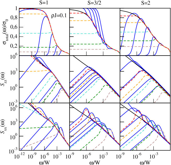
Figure 10: (Color online) Dynamic properties of the anisotropic Kondo model. We plot the spectral function of the $T$-matrix (“conductance”) and the longitudinal and transversal dynamical suspectibility $\mathcal{S}_{\mathrm{zz}}(\omega)$ and $\mathcal{S}_{\mathrm{xx}}(\omega)$. The curves correspond to $|D|=10^{-2},\ldots,10^{-6}$; the curve styles are the same as in Fig. 2. Note that for $S=2$ and $D=10^{-6}$ the susceptibility curves do not diverge; they start decreasing at an energy scale outside the displayed range.

In the hard-axis $D>0$ case, the conductance at low temperatures is zero for all integer values of the impurity spin, while it is unitary for all half-integer spins. For $S=1$ and $D<T_{K}^{(0)}$, this can be explained by the two-stage Kondo screening: the first $S=1$ screening stage leads to increased conductance as in the isotropic case, however the conductance drops to zero at a lower temperature scale $T_{K}^{(2)}$ when the residual spin-$1/2$ is compensated in the second screening stage. This is similar to the screening of a $S=1$ impurity by two conduction channels with unequal exchange constants Nozières and Blandin (1980); Sasaki et al. (2000), but here the two-stage screening occurs with a single channel. Non-monotonous energy-dependence of the spectral function is also found in the case of side-coupled impurities, but there both screening stages are of the $S=1/2$ kind Vojta et al. (2002a); Cornaglia and Grempel (2005); Žitko and Bonča (2006); Chung et al. (2008). For large $D>T_{K}^{(0)}$, the anisotropy makes the impurity non-magnetic, there is no exchange scattering at energy scales below $D$ and the low-temperature conductance drops to zero. Note that in both cases the stable fixed point is the same, the ratio $D/T_{K}^{(0)}$ merely determines by which mechanism the $S=1$ Kondo screening is interrupted by the anisotropy; the transition between the two regimes is smooth.

For higher integer spins (represented in Fig. 10 by the $S=2$ case), the situation is in some respect similar. For $D<T_{K}^{(0)}$, the conductance at first increases during the initial spin-$S$ Kondo screening, there is even a slight bump above the result for the isotropic case on the energy scale of $D$ when the effective spin doublet is formed and there is additional resonantly enhanced scattering. Spin-$S$ Kondo screening yields a half-integer effective impurity spin, thus a spin-$1/2$ doublet on the energy scale $D$. The spin-$1/2$ Kondo screening then leads to a decrease in conductance to zero. As previously discussed, the main difference from the $S=1$ case is that there is no exponential reduction of the energy scale for $D<T_{K}^{(0)}$.

For half-integer spins (represented in Fig. 10 by the $S=3/2$ case), the conductance at low temperatures is unitary, as in the isotropic case. For $D>T_{K}^{(0)}$, this may be explained by the fact that the anisotropy leads in this case to a low-laying doublet formed by the $S_{z}=\pm 1/2$ magnetic doublet which undergoes Kondo screening like in the conventional spin-$1/2$ Kondo model. The doublet is formed before the spin-$S$ Kondo screening commences and the mapping to the spin-$1/2$ Kondo model is a good approximation: the Kondo resonance then has approximately Lorentzian form. It may be noted that there is again an additional peak in $\sigma(\omega)$ at $\omega\sim D$ due to resonantly enhanced scattering by the $S_{z}\to S_{z}\pm 1$ processes. For $D<T_{K}^{(0)}$, the conductance curve first follows the logarithmically increasing isotropic spin-$S$ curve, then at $D$ the approach to the unitary limit becomes faster.

We emphasize the marked difference between the integer spin $S=2$ and the half-integer spin $S=3/2$ regarding the energy scale where the limiting value of $\sigma_{\mathrm{total}}$ ($0$ viz. $1$) is approached: for $S=2$, the characteristic frequency decreases faster than linearly with $D$ for small $D$, while for $S=3/2$ it tends to increase very slowly with $D$ for large $D$. In both cases this behavior is due to the underlying effective $S=1/2$ Kondo physics; for $S=2$ it implies that the effective exchange constant becomes smaller as $D$ is reduced, while for $S=3/2$ this is due to the saturation of the effective $J_{\perp}/J_{z}$ ratio for large $D$ as already discussed.

We now consider the easy-axis $D<0$ case. For all $S$, the conductance is found to saturate at some $D$-dependent finite value here. This reflects the presence of a residual uncompensated impurity spin which induces scattering at low temperatures which is neither unitary nor zero (these are the only two possibilities compatible with a Fermi-liquid system in the presence of the particle-hole symmetry which imposes the restriction $\delta\equiv-\delta\mod\pi$ on the quasiparticle scattering phase shift $\delta$, thus $\delta=0$ or $\delta=\pi$). This implies that the stable fixed point may be classified as a non-Fermi liquid, which is confirmed by the non-vanishing inelastic scattering rate at the Fermi level, see Fig. 11. In the limit $|D|\to 0$, this non-Fermi-liquid fixed point evolves continuously into a singular Fermi-liquid fixed point of the isotropic underscreened Kondo model. Since the approach to this limit is slow (in particular for $S\geq 3/2$), even very small negative axial anisotropy will lead to significantly reduced conductance at low temperatures. In the following we show that this behavior is modified by non-zero $E$ (see also Ref. Romeike et al., 2006a). Nevertheless, if $E\ll|D|$, there might exist a temperature range where the non-Fermi-liquid behaviour is observable.

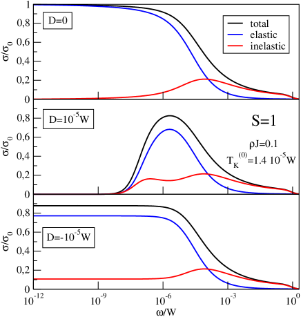
Figure 11: (Color online) Total, elastic and inelastic scattering cross sections for the $S=1$ Kondo model with no anisotropy, positive anisotropy and negative anisotropy.

We now consider the imaginary part of the dynamic spin susceptibility $\mathcal{S}_{\alpha\alpha}(\omega)$. We recall that these quantities are given at zero temperature by

$$\mathcal{S}_{\alpha\alpha}(\omega)=-\frac{1}{\pi}\frac{1}{Z_{N}}\sum_{i,j_{\mathrm{GS}}}|\langle i|S_{\alpha}|j_{\mathrm{GS}}\rangle|^{2}\delta\left(\omega-(E_{i}-E_{\mathrm{GS}})\right)$$ (26)

where the index $i$ runs over the excited states and the index $j_{\mathrm{GS}}$ over the degeneracy of the ground state, while $Z_{N}$ is the zero-temperature partition function (equal to the degeneracy of the ground state). In the absence of the coupling to the conduction band, the transverse susceptibility $\mathcal{S}_{xx}(\omega)$ features delta peak(s) at

$$\omega=|DS_{z}^{2}-D(S_{z}-1)^{2}|=|D(2S_{z}-1)|,$$ (27)

since $S_{x}$ couples neighboring levels. For $S=1$, there is thus a peak at $|D|$, for $S=3/2$ a peak at $2|D|$ and for $S=2$, depending on the sign of $D$, a peak at $D$ (for $D>0$) or at $3|D|$ (for $D<0$). The longitudinal susceptibility $\mathcal{S}_{zz}(\omega)$ of a decoupled impurity is zero.

The $S=1$ case has some special features, so we focus first on the regular cases, $S\geq 3/2$. The longitudinal susceptibility $\mathcal{S}_{zz}(\omega)$ always has a single peak. In the hard-axis $D>0$ case we find that the peak occurs at the energy scale of the effective $S=1/2$ Kondo effect (when it occurs, i.e. $D>T_{K}^{(0)}$ for $S=3/2$ and $D<T_{K}^{(0)}$ for $S=2$, respectively) or at $\sim D$ in the regime with no $S=1/2$ Kondo effect. In both cases this corresponds to the energy scale where the conductance approaches its limiting value, as discussed above. This result is expected, since in the presence of the Kondo effect the largest magnetic fluctuations always occur on the energy scale of $T_{K}$, which is a reflection of the anomalously strong spin-flip scattering of the conduction band electrons off the impurity; in the absence of the Kondo effect, magnetic fluctuations occur on the scale of the local magnetic excitation energy, in this case the anisotropy $D$. In the easy-axis $D<0$ case, the position of the peak in $\mathcal{S}_{zz}(\omega)$ is always $\sim|D|$.

For all $D$ and all $S\geq 3/2$, the approach to the zero frequency limit is linear, while the behavior at high frequencies is described approximately by a power law $\mathcal{S}(\omega)\sim\omega^{-\gamma}$ with exponents $\gamma$ that are slightly above 1 Costi (1998).

The transverse susceptibility $\mathcal{S}_{xx}(\omega)$ is more complex. In the hard-axis $D>0$ case, we find a two-peak behavior in the parameter regime with $S=1/2$ Kondo effect: the first peak corresponds to the scale of $D$, the second to the scale of $T_{K}$. In the transition regime $D\sim T_{K}^{(0)}$, the two peaks merge into a single peak which then follows the scale of anisotropy $D$. In the easy-axis $D<0$ case, the curves again have a single peak at $\sim|D|$. At this point a comment on the peak width is in order: the peaks at $\sim|D|$ are over-broadened due to the broadening procedure used in the NRG method, thus the very narrow peaks take the form of the broadening kernel Garst et al. (2005).

We now finally turn to $S=1$. For hard-axis $D>0$ anisotropy, we find for both $\mathcal{S}_{zz}(\omega)$ and $\mathcal{S}_{xx}(\omega)$ a single peak centered at $\omega\sim D$ (for $D>T_{K}^{(0)}$) or at $\omega\sim T_{K}^{(2)}$ (for $D<T_{K}^{(0)}$). In $\mathcal{S}_{xx}(\omega)$, there is no additional peak on the scale of $D$ for $D<T_{K}^{(0)}$, as was the case for the spin-$2$ model, but we observe a change of slope at $\omega\sim T_{K}^{(0)}$. Even more peculiar are the results for the easy-axis $D<0$ case. The longitudinal susceptibility has a linear frequency dependence for $|D|\gtrsim T_{K}^{(0)}$, but for $|D|\lesssim T_{K}^{(0)}$ we observe $\omega^{\alpha}$ scaling with exponent $\alpha$ which depends on the anisotropy $D$ and which turns negative approximately at $|D|\sim T_{K}^{(0)}$, i.e. the susceptibility becomes divergent. In the transverse susceptibility we find a strong deviation from linear scaling for all values of $|D|$, with divergent behavior already for $|D|$ much larger than $T_{K}^{(0)}$. We emphasize that for all spin values $S$, the easy-axis $D<0$ systems exhibit non-Fermi-liquid features (such as finite inelastic scattering at $\omega=0$), but only for $S=1$ is the dynamic spin susceptibility divergent at low frequencies.

We note that a linear frequency dependence of $\mathcal{S}_{\alpha\alpha}(\omega)$ at low frequencies must hold in Fermi-liquid systems as mandated by the Korringa-Shiba relations Shiba (1975); Costi and Kieffer (1996); Hofstetter and Kehrein (2001); Garst et al. (2005). For $D<0$ the system is, however, non-Fermi liquid and the static magnetic susceptibility is diverging for all $S$, thus $\mathcal{S}(\omega)$ is not expected to be linear. We view the fact that it is linear for $S\geq 3/2$ merely as a coincidence.

We finish our discussion of dynamic properties by showing that in the presence of the transverse anisotropy term $E(S_{x}^{2}-S_{y}^{2})$, all non-Fermi-liquid features disappear, Fig. 11. In particular, we observe that for all integer $S$ the low-temperature conductance is zero, while for all half-integer $S$ it is unitary, irrespective of the sign and size of the axial anisotropy $D$. Furthermore, the spin susceptibility always has linear frequency dependence at low frequencies. This agrees with the results for static properties.

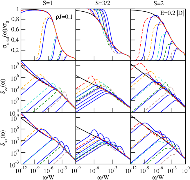
Figure 12: (Color online) Dynamic properties of the anisotropic Kondo model with the $E(S_{x}^{2}-S_{y}^{2})$ term. $E=0.2|D|$. The curve styles are the same as in Fig. 2.

V Conclusion

Due to the presence of the magnetic anisotropy, the impurity spin is always completely compensated at low enough temperature, even in the case of high-spin impurities coupled to a single continuum channel. This goes against the common wisdom that a single channel can screen at most $1/2$ unit of spin, which results in a residual spin of $S-k/2$ in the case of $k$ screening channels: such a behavior will only be observable for isotropic systems, a situation which is rather unlikely for magnetic impurities adsorbed on surfaces.

The approach to the fully screened impurity spin with decreasing energy scale depends on the impurity spin $S$, the sign of axial anisotropy $D$, and on the hierarchy of the energy scales, in particular on the dichotomy $D<T_{K}^{(0)}$ or $D>T_{K}^{(0)}$ in the positive-$D$ models. For positive $D$ (hard-axis case), we find spin-$1/2$ Kondo screening at low temperatures in the weak-anisotropy case $D<T_{K}^{(0)}$ for integer spin (with exponentially reduced Kondo temperature in the special case of spin 1) and in the strong-anisotropy case $D>T_{K}^{(0)}$ for half-integer spin; in other cases, the effective impurity moment drops to zero exponentially on the energy scale of $D$. The transverse anisotropy $E$ does not play an important role for $D>0$. For negative $D$ (easy-axis case), however, it changes the behavior of the system completely. For $E=0$, the impurity spin would be only partially screened, leading to residual spin-dependent scattering and non-Fermi-liquid behavior. In real systems $E\neq 0$ and the behavior of $D<0$ becomes similar to that of the $D>0$ systems: for $S=1$ we again find two-stage Kondo screening for $E<T_{K}^{(0)}$, for $S=3/2$ there is effective spin-$1/2$ Kondo effect for $E>T_{K}^{(0)}$, while for $S=2$ we find effective spin-$1/2$ screening for $E<T_{K}^{(0)}$. If $E\ll|D|$, some features of the non-Fermi-liquid behavior might be observable in intermediate temperature respectively energy regimes. The zero-temperature conductance is found to be zero for all integer spins and unitary for all half-integer spins for both signs of $D$ (assuming $E\neq 0$). For integer spin and $E,D<T_{K}^{(0)}$, the temperature dependence of the conductance is expected to be non-monotonous with increased conductance in the $T_{K}(S=1/2)<T<T_{K}^{(0)}$ range. The most likely candidate for observation of underscreening is the $S=1$ case due to the exponential reduction of the second Kondo temperature, which is a special feature of the $S=1$ model and is not found for other integer spins.

We conclude by noting that taking the magnetic anisotropy effects into account is essential in interpreting scanning tunneling spectra of magnetic impurities measured at low temperatures ($T\ll|D|$). The appropriate low-temperature effective impurity model depends on the parameters of the original physical model. While most interpretations of the surface Kondo effect have been based on the Anderson impurity model (which maps on the isotropic Kondo model), it is more likely that the appropriate effective model is, in fact, some anisotropic Kondo model. This is especially true for impurities on decoupling layers, but also applies to impurities adsorbed directly on metallic surface where due to stronger hybridisation charge fluctuation effects also play a role. Appropriate description in terms of an anisotropic model has important consequences on the relation between the Kondo temperature and the “bare” model parameters (effective bandwidth, exchange constants $J_{\perp}$ and $J_{z}$), and on the coupling of the effective impurity spin with the external magnetic field.

Appendix A Analysis of the non-Fermi-liquid fixed point

We study the properties of the non-Fermi-liquid fixed point in the $S=1$ Kondo model with $D<0$ in the extreme anisotropic limit, $|D|\to\infty$ (numerical results, where needed, are taken from a $D=-100W$ calculation).

We show that in the $N\to\infty$ limit ($N$ being the NRG iteration number), the fixed point corresponds to fermions with residual anisotropic exchange scattering from a $S_{z}=\pm 1$ magnetic doublet. In other words, there is no decoupling of the residual impurity spin, as in the isotropic $S=1$ Kondo model Koller et al. (2005). There is furthermore no effective potential scattering in the $|D|\to\infty$ limit, since the conduction band electrons cannot flip the impurity spin due to the high energy barrier, thus there can be no quasiparticle phase shift due to Kondo screening. We may thus take the Hamiltonian for the uncoupled conduction band chain Koller et al. (2005)

$$H_{\mathrm{band}}=\xi^{-1}\Lambda^{-(N-1)/2}\sum_{r}\left(E_{p}^{(0)}p^{\dagger}_{r,\sigma}p_{r,\sigma}+E_{h}^{(0)}h^{\dagger}_{r,\sigma}h_{r,\sigma}\right),$$ (28)

where $p$ and $h$ are second quantization operators for particle and hole excitations, while $E_{p}^{(0)}$ and $E_{h}^{(0)}$ are their energies in the units of the characteristic energy scale at the $N$-th NRG iteration, and $\xi=\ln\Lambda\sqrt{\Lambda}/(1-\Lambda^{-1})\approx 2.41$ is an additional scale factor in the discretization scheme used in this work Campo and Oliveira (2005).

The fixed-point Hamiltonian can be written as $H^{\prime}=H_{\mathrm{band}}+H_{c}$ with

$$H_{c}=J^{*}_{z}s_{z}S_{z}+J^{*}_{\perp}\left(s_{x}S_{x}+s_{y}S_{y}\right),$$ (29)

where $s_{i}$ are the spin operators on the first site of the Wilson chain,

$$s_{i}=\sum_{\alpha\alpha^{\prime}}f^{\dagger}_{0,\alpha}\left(\frac{1}{2}\sigma^{i}_{\alpha\alpha^{\prime}}\right)f_{0,\alpha^{\prime}},$$ (30)

while $S_{i}$ are the impurity spin-$1$ operators. The $f_{0}$ operators need to be written in terms of the single particle and hole operators Wilson (1975):

$$f^{\dagger}_{0\sigma}=\sum_{r}\alpha_{0r}\left(p^{\dagger}_{r,\sigma}+h_{r,\sigma}\right).$$ (31)

In the $|D|\to\infty$ limit, the Hilbert space is restricted to the $S_{z}=\pm 1$ states, thus the transverse exchange $J^{*}_{\perp}$ drops out. Keeping only the terms involving the particle excitations, we finally obtain

$$H_{c}=J^{*}_{z}\sum_{r,r^{\prime}}\alpha_{0r}\alpha_{0r^{\prime}}S_{z}\frac{1}{2}\left(p^{\dagger}_{r,\uparrow}p_{r^{\prime},\uparrow}-p^{\dagger}_{r,\downarrow}p_{r^{\prime},\downarrow}\right).$$ (32)

Energy	$Q$	$S_{z}$	Degeneracy
0	$0$	$\pm 1$	2
0.672864	$\pm 1$	$\pm 1/2$	4
0.820964	$\pm 1$	$\pm 3/2$	4
1.345728	$0$	$0$	2
1.493829	$\pm 2,0[\times 2]$	$\pm 1$	8
1.641929	$0$	$\pm 2$	2

Table 1: Excitation spectrum for large negative $D$ (here $D=-100W$, $\Lambda=2.5$, $N=79$). The lowest single-particle excitations for free electrons is $E_{p,1}^{(0)}=0.7468559$.

The fixed-point excitation spectrum computed using NRG is shown in Table 1. The ground state has total charge $Q=0$ and consists of two spin states $S_{z}=\pm 1$. There are four low-lying single-particle excited states with $Q=+1$: two degenerate levels with $S_{z}=\pm 1/2$ and (scaled) energy

$$E_{p}(A)=E_{p,1}^{(0)}-\frac{1}{2}J^{*}_{z}\alpha_{01}^{2}\Lambda^{(N-1)/2}\xi$$ (33)

and two other degenerate levels with $S_{z}=\pm 3/2$ and energy

$$E_{p}(B)=E_{p,1}^{(0)}+\frac{1}{2}J^{*}_{z}\alpha_{01}^{2}\Lambda^{(N-1)/2}\xi$$ (34)

In the first two levels, the impurity spin and the spin of the particle excitation are anti-aligned, while in the second two levels the impurity spin and the spin of the particle are aligned.

Since the energy difference between $E_{p}(A)$ and $E_{p}(B)$ no longer varies with $N$ at the fixed point and the factor ${\overline{\alpha}}_{01}^{2}=\alpha_{01}^{2}\Lambda^{(N-1)/2}$ reaches its limiting value (equal to $0.309$ for $\Lambda=2.5$) this implies that $J^{*}_{z}$ is a constant given by

$$J^{*}_{z}=\frac{E_{p}(B)-E_{p}(A)}{\overline{\alpha}_{01}^{2}\xi}.$$ (35)

For $\rho J=0.1$ and $D=-100W$ (Table 1) we obtain

$$J^{*}_{z}\approx 0.198W=0.99J.$$ (36)

As expected, we obtain $J^{*}_{z}$ which is essentially equal to the bare $J$ in the large-$|D|$ limit.