Time-Delayed Feedback in Neurosystems

Abstract

The influence of time delay in systems of two coupled excitable neurons is studied in the framework of the FitzHugh-Nagumo model. Time-delay can occur in the coupling between neurons or in a self-feedback loop. The stochastic synchronization of instantaneously coupled neurons under the influence of white noise can be deliberately controlled by local time-delayed feedback. By appropriate choice of the delay time synchronization can be either enhanced or suppressed. In delay-coupled neurons, antiphase oscillations can be induced for sufficiently large delay and coupling strength. The additional application of time-delayed self-feedback leads to complex scenarios of synchronized in-phase or antiphase oscillations, bursting patterns, or amplitude death.

I Introduction

Control of unstable or irregular states of nonlinear dynamic systems is a central issue of current research SCH07 . A particularly simple and efficient control scheme is time-delayed feedback which occurs naturally in a number of biological systems including neural networks where both propagation delays of electrical signals connecting different neurons and local neurovascular couplings lead to time delays HAK06 ; WIL99 ; GER02 . Moreover, time-delayed feedback loops might be deliberately implemented to control neural disturbances, e.g., to suppress undesired synchrony of firing neurons in Parkinson’s disease or epilepsy SCH94e ; ROS04a ; POP05 . Chaos control techniques have been first applied experimentally in vitro in a spontaneously bursting neural network SCH94e using a method proposed by Ott, Grebogi and Yorke OTT90 . In contrast to this method, the time-delayed feedback method by Pyragas PYR92 and its extensions SOC94 do not require detailed information on the system to be controlled, and they are non-invasive, i. e., once the target state is reached, the control force vanishes. However, one needs to tune the feedback gain and the delay time. Therefore, theoretical investigations help to understand optimal choices of these parameters. Various global delayed feedback schemes have been proposed as effective and robust therapy of neurological diseases with pathological synchronization causing tremor ROS04a ; POP05 . They have been contrasted with local delayed feedback methods GAS07b ; GAS08 ; DAH08 .

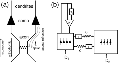
Figure 1: (a) Scheme of two axo-axonally coupled neurons (pyramidal cells coupled by an electrical synapse) SCH01e . (b) Two mutually coupled neural populations (delay $\tau$, coupling constant $C$) with feedback control loop (delay $\tau_{K}$, coupling constant $K$) and noise input $D_{1}$, $D_{2}$.

Neurons are excitable units which can emit spikes or bursts of electrical signals, i.e., the system rests in a stable steady state, but after it is excited beyond a threshold, it emits a pulse. In the following, we consider electrically coupled neurons. Such electrical synapses are less common than chemical synapses, but it has been shown in hippocampal slices that high-frequency synchronized oscillations are independent of chemical synaptic transmission JEF82 , and physiological, pharmacological, and structural evidence was provided SCH01e that axons of hippocampal pyramidal cells are electrically coupled (Fig. 1 (a)). Time delays in the coupling must be considered particularly in the case of high-frequency oscillations.

The simplest model that displays features of neural interaction consists of two coupled neural systems. A single electrical synapse can lead to synchronized co-operative behaviour between two axo-axonally coupled hippocampal pyramidal cells when only one of them is stimulated antidromically at high frequency TRA94 ; TRA99 . Moreover, such neurons have been shown to reflect antidromic spikes (propagating opposite to the normal direction) at the soma, but a continuous reverberating activity is not generated by axonal reflections in two axo-axonally coupled cells alone SCH01e . In order to describe the complicated interaction between billions of neurons in large neural networks, the neurons are often lumped into highly connected sub-networks or synchronized sub-ensembles. Such neural populations are usually localized spatially and contain both excitatory and inhibitory neurons WIL72 . In this sense, the model of two mutually coupled neurons may also serve as a paradigm of two coupled neural sub-ensembles.

Starting from such simplest network motifs, larger networks can be built, and their effects may be studied. For example, starting from two interconnected reticular thalamic neurons with oscillatory behavior, it was shown in DES94 how more complex dynamics emerges in ring networks with nearest neighbors and fully reciprocal connectivity, or in networks organized in a two-dimensional array with proximal connectivity and “dense proximal” coupling in which every neuron connects to all other neurons within some radius. In another example ZHO06c , a neural population was itself modeled as a small sub-network of excitable elements, to study hierarchically clustered organization of excitable elements in a network of networks.

In the following, we consider two mutually coupled neurons modelled by the paradigmatic FitzHugh-Nagumo system FIT61 ; NAG62 ; LIN04 in the excitable regime:

$$\epsilon_{1}\dot{x}_{1} = x_{1}-\frac{x_{1}^{3}}{3}-y_{1}+C[x_{2}(t-\tau)-x_{1}(t)]$$

$$\dot{y}_{1} = x_{1}+a+D_{1}\xi_{1}(t)$$

$$\epsilon_{2}\dot{x}_{2} = x_{2}-\frac{x_{2}^{3}}{3}-y_{2}+C[x_{1}(t-\tau)-x_{2}(t)]$$

$$\dot{y}_{2} = x_{2}+a+D_{2}\xi_{2}(t)$$ (1)

where $x_{1},y_{1}$ and $x_{2},y_{2}$ correspond to single neurons (or neuron populations), which are linearly coupled with coupling strength $C$. The variables $x_{1}$, $x_{2}$ are related to the transmembrane voltage and $y_{1}$, $y_{2}$ refer to various quantities connected to the electrical conductance of the relevant ion currents. Here $a$ is an excitability parameter whose value defines whether the system is excitable ($a>1$) or exhibits self-sustained periodic firing ($a<1$), $\epsilon_{1}$ and $\epsilon_{2}$ are the timescale parameters that are usually chosen to be much smaller than unity, corresponding to fast activator variables $x_{1}$, $x_{2}$, and slow inhibitor variables $y_{1}$, $y_{2}$.

The synaptic coupling between two neurons is modelled as a diffusive coupling considered for simplicity to be symmetric LIL94 ; PIN00 ; DEM01 . More general delayed couplings are considered in BUR03 . The coupling strength $C$ summarizes how information is distributed between neurons. The mutual delay $\tau$ in the coupling is motivated by the propagation delay of action potentials between the two neurons $x_{1}$ and $x_{2}$.

Each neuron is driven by Gaussian white noise $\xi_{i}(t)$ $(i=1,2)$ with zero mean and unity variance. The noise intensities are denoted by parameters $D_{1}$ and $D_{2}$, respectively.

Besides the delayed coupling we will also consider delayed self-feedback in the form suggested by Pyragas PYR92 , where the difference $s(t)-s(t-\tau_{K})$ of a system variable $s$ (e.g., activator or inhibitor) at time $t$ and at a delayed time $t-\tau_{K}$, multiplied by some control amplitude $K$, is coupled back into the same system (Fig. 1(b)). Such feedback loops might arise naturally in neural systems, e.g., due to neurovascular couplings that has a characteristic latency, or due to finite propagation speed along cyclic connections within a neuron sub-population, or they could be realized by external feedback loops as part of a therapeutical measure, as proposed in Ref. POP05 . This feedback scheme is simple to implement, quite robust, and has already been applied successfully in a real experiment with time-delayed neurofeedback from real-time magnetoencephalography (MEG) signals to humans via visual stimulation in order to suppress the alpha rhythm, which is observed due to strongly synchronized neural populations in the visual cortex in the brain HAD06 . One distinct advantage of this method is its non-invasiveness, i.e., in the ideal deterministic limit the control force vanishes on the target orbit, which may be a steady state or a periodic oscillation of period $\tau$. In case of noisy dynamics the control force, of course, does not vanish but still remains small, compared to other common control techniques using external periodic signals, for instance, in deep-brain stimulation to suppress neural synchrony in Parkinson’s disease TAS02 .

The phase portrait and the null-isoclines of a single FitzHugh-Nagumo system without noise and feedback are shown in Fig. 2(a). The fixed point A is a stable focus or node for $a>1$ (excitable regime). If the system is perturbed well beyond point A’ (see inset), it performs a large excursion $A\to B\to C\to D\to A$ in phase space corresponding to the emission of a spike (Fig. 2(b)). At $a=1$ the system exhibits a Hopf bifurcation of a limit cycle, and the fixed point A becomes an unstable focus for $a<1$ (oscillatory regime).

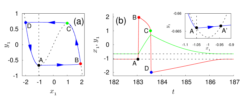
Figure 2: Excitable dynamics of a single FitzHugh-Nagumo system: (a) Phase portrait $(x_{1},y_{1})$ (trajectory: solid blue, nullclines: dashed black), (b) Time series of activator $x_{1}(t)$ (red) and inhibitor $y_{1}(t)$ (green). The colored dots A, B, C, D mark corresponding points on panels (a) and (b). The inset in (b) shows a blow-up of the phase portrait near A. Parameters: $\epsilon_{1}=0.01$, $a=1.05$, $D_{1}=0$.

In the following we choose the excitability parameter $a=1.05$ in the excitable regime close to threshold. If noise is present, it will occasionally kick the system beyond $A^{\prime}$ resulting in noise-induced oscillations (spiking).

II Stochastic synchronization of instantaneously coupled neurons

We shall first consider two coupled FitzHugh-Nagumo systems as in eq. (I) albeit without delay in the coupling ($\tau=0$). Noise can induce oscillations even though the fixed point is stable HAU06 ; HOE07 . The noise sources then play the role of stimulating the excitable subsystems. Even if only one subsystem is driven by noise, it induces oscillations of the whole system through the coupling. In the following, we consider two nonidentical neurons, described by different timescales $\epsilon_{1}=0.005$, $\epsilon_{2}=0.1$, and set the noise intensity $D_{2}$ in the second subsystem equal to a small value, $D_{2}=0.09$, in order to model some background noise level. Depending on the coupling strength $C$ and the noise intensity $D_{1}$ in the first subsystem, the two neurons show cooperative dynamics.

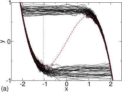
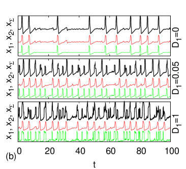
Figure 3: (a): Noise-induced oscillations in a single FitzHugh-Nagumo system ($C=0$) for a noise intensity $D_{1}=0.6$. The red dashed and dash-dotted lines denote the null-isoclines. Panel (b): Time series of two instantaneously coupled FitzHugh-Nagumo systems for different noise intensities $D_{1}$. The green (light grey), red (dark grey), and black curves correspond to $x_{1}$, $x_{2}$, and their sum $x_{\Sigma}=x_{1}+x_{2}$, respectively. Other parameters: $a=1.05$, $\epsilon_{1}=0.005$, $\epsilon_{2}=0.1$, $\tau=0$, $C=0.07$ and $D_{2}=0.09$.

Figure 3(a) depicts the temporal dynamics of a single FitzHugh-Nagumo system ($C=0)$ due to stochastic input. One can see that the system is excitable since it performs large excursions in phase space. Figure 3(b) shows the temporal dynamics of the two instantaneously coupled neural systems for increasing noise intensities $D_{1}$, where the green (light grey), red (dark grey), and black curves correspond to $x_{1}$, $x_{2}$, and their sum $x_{\Sigma}=x_{1}+x_{2}$, respectively. For $D_{1}=0$, the first subsystem is enslaved and emits a spike every time the second unit does. For increasing $D_{1}$, however, this synchronization is weakened and for large noise intensities $D_{1}$ the dynamics of the first subsystem is independently dominated by its own stochastic input.

There are various measures of the synchronization of coupled systems ROS01a . For instance, one can consider the average interspike intervals of each subsystem, i.e. $\langle T_{1}\rangle$ and $\langle T_{2}\rangle$, calculated from the $x$ variable of the respective subsystem. Their ratio $\langle T_{1}\rangle/\langle T_{2}\rangle$ is a measure of frequency synchronization, as depicted in Fig. 4. Panel (a) displays the ratio of average interspike intervals in dependence on the noise intensity $D_{1}$ (green dots) for fixed coupling strength $C=0.07$. One can see that for increasing $D_{1}$ the ratio $\langle T_{1}\rangle/\langle T_{2}\rangle$ decreases. Thus, the two subsystems become less synchronized. Panel (b) shows the dependence on the coupling strength $C$ for fixed noise intensity $D_{1}=0.25$. Without coupling ($C=0$), the two subsystems operate on their own timescale. For increasing $C$, however, they synchronize as the ratio of the average interspike intervals approaches unity. Panel (c) shows the result as a function of $D_{1}$ and $C$, where the bright regions indicate a strongly synchronized behaviour of the two subsystems. For small $D_{1}$ and large coupling strength $C$, the two subsystems display synchronized behaviour, $\langle T_{1}\rangle/\langle T_{2}\rangle\approx 1$. On average, they show the same number of spikes indicated by bright (yellow) color. In the next Section, we consider three different regimes of synchronization: moderately, weakly, and strongly synchronized systems as marked by black dots in Fig. 4(c).

Other measures for stochastic synchronization are given by the phase synchronization index HAU06 , or the mean phase synchronization intervals HOE08 , but they exhibit qualitatively similar behaviour.

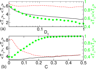
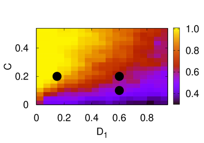
Figure 4: Frequency synchronization: Average interspike intervals of each subsystem (black solid curve: $\langle T_{1}\rangle$, red dashed: $\langle T_{2}\rangle$) and their ratio (green dotted: $\langle T_{1}\rangle/\langle T_{2}\rangle$) (a) vs. noise intensity $D_{1}$ (for fixed $C=0.07$), (b) vs. coupling strength $C$ (for fixed $D_{1}=0.25$). (c): Ratio of the average interspike intervals in the ($D_{1},C$) plane. The black dots mark the parameter choices for different synchronization regimes used in Fig. 5. Other parameters: $a=1.05$, $\epsilon_{1}=0.005$, $\epsilon_{2}=0.1$, $\tau=0$, and $D_{2}=0.09$.

III Control of synchronization by time-delayed feedback

In this Section, we consider the control of global cooperative dynamics by local application of a stimulus to a single system. This stimulus is realized by time-delayed feedback, which was initially introduced by Pyragas in order to stabilize periodic orbits in deterministic systems PYR92 :

$$\epsilon_{1}\dot{x}_{1} = x_{1}-\frac{x_{1}^{3}}{3}-y_{1}+C[x_{2}(t)-x_{1}(t)]$$ (2a)

$$\dot{y}_{1} = x_{1}+a+K\left[y_{1}(t-\tau_{K})-y_{1}(t)\right]+D_{1}\xi_{1}(t)$$

$$\epsilon_{2}\dot{x}_{2} = x_{2}-\frac{x_{2}^{3}}{3}-y_{2}+C[x_{1}(t)-x_{2}(t)]$$ (2b)

$$\dot{y}_{2} = x_{2}+a+D_{2}\xi_{2}(t).$$

The parameters of the time-delayed feedback scheme are the feedback gain $K$ and the time delay $\tau_{K}$. With this method, a control force is constructed from the differences of the states of the system which are one time unit $\tau_{K}$ apart. One could also consider application of the feedback scheme to both subsystems and effects of different values of the control parameters for each subsystem, but these investigations are beyond of the scope of this work. Previously, time-delayed feedback has also been used to influence noise-induced oscillations of a single excitable system JAN03 ; BAL04 ; PRA07 , of systems below a Hopf bifurcation SCH04b ; POM05a ; POT07 ; FLU07 or below a global bifurcation HIZ06 ; HIZ08 , and of spatially extended reaction-diffusion systems STE05a ; BAL06 ; DAH08 . Extensions to multiple time-delay control schemes have also been considered POM07 ; SCH08a ; HOE07 ; HOE08 .

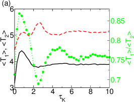
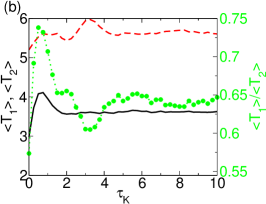
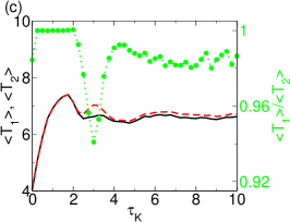
Figure 5: Control of synchronization: Interspike intervals vs. time delay $\tau_{K}$. Green dots: ratio of the interspike intervals $\langle T_{1}\rangle/\langle T_{2}\rangle$ of the two subsystems, black solid curve: $\langle T_{1}\rangle$, red dashed curve: $\langle T_{2}\rangle$. Panels (a), (b), and (c) correspond to the case of moderate ($C=0.2$, $D_{1}=0.6$), weak ($C=0.1$, $D_{1}=0.6$), and strong ($C=0.2$, $D_{1}=0.15$) synchronization, respectively. Other parameters: $a=1.05$, $\epsilon_{1}=0.005$, $\epsilon_{2}=0.1$, $C=0.07$, $\tau=0$, $D_{2}=0.09$, $K=1.5$.

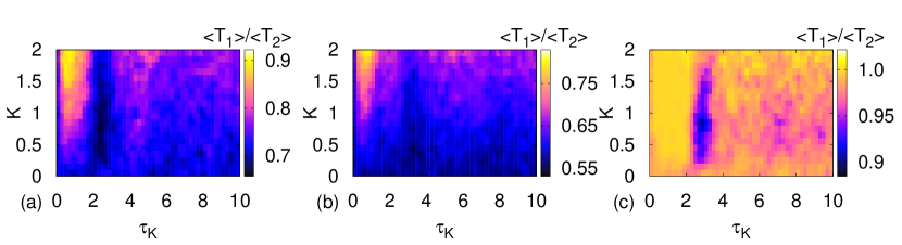
Figure 6: Ratio of interspike intervals $\langle T_{1}\rangle/\langle T_{2}\rangle$ in dependence on the feedback gain $K$ and the time delay $\tau$ for (a) moderate ($C=0.2$, $D_{1}=0.6$), (b) weak ($C=0.1$, $D_{1}=0.6$), and (c) strong ($C=0.2$, $D_{1}=0.15$) synchronization. Other parameters as in Fig. 4(c).

Since we are interested in the effects of a control force on the synchronization, in the following we consider three different cases: moderately, weakly, and strongly synchronized systems given by the specific choices of the coupling strength and noise intensity in the first subsystem. These different cases of stochastic synchronization are marked as black dots in Fig. 4.

As a measure to quantify changes in the synchronization due to the control force, we consider the ratio of average interspike intervals. In the presence of a control force, i.e., $K\neq 0$, the cooperativity can be influenced by varying the feedback gain $K$ and the time delay $\tau_{K}$.

For fixed feedback gain $K=1.5$, Fig. 5 depicts the average interspike intervals of the subsystems, shown as solid (black) and dashed (red) curves for $\langle T_{1}\rangle$ and $\langle T_{2}\rangle$, and their ratio (green dots) for the case of (a) moderately, (b) weakly, and (c) strongly synchronized systems, respectively, in dependence on the time delay $\tau_{K}$. In all three cases, the stochastic synchronization can be strongly modulated by changing the delay time, i.e., one can either enhance and suppress synchronization by appropriate choice of the local feedback delay.

The overall dependence of the frequency synchronization, measured by the ratio of $\langle T_{1}\rangle/\langle T_{2}\rangle$, is displayed in dependence on the control parameters $K$ and $\tau_{K}$ in Fig. 6 for moderate, weak, strong synchronization in panels (a), (b), and (c), respectively. Thus, Fig. 5 can be understood as a horizontal cut for $K=1.5$ through Fig. 6. One can see a modulation of the ratio of average interspike interval by $\tau_{K}$ for a large range of feedback gain. In view of applications, where neural synchronization is often pathological, e.g. in Parkinson’s disease or epilepsy, it is interesting to note that there are cases where a proper choice of the local feedback control parameters leads to desynchronization of the coupled system (dark regions in Fig. 6).

IV Delay-coupled neurons

In this section we study the influence of a delay in the coupling of two neurons, rather than a delayed self-feedback. We set the noise terms in Eq. (I) equal to zero, $D_{1}=D_{2}=0$, but consider a time-delay $\tau$ in the coupling. In the deterministic system the delayed coupling plays the role of a stimulus which can induce self-sustained oscillations in the coupled system even if the fixed point is stable. In this sense the delayed coupling has a similar effect as the noise term in the previous sections. Here the bifurcation parameters for delay-induced bifurcations are the coupling parameters $C$ and $\tau$.

IV.1 Linear stability of fixed point

In the following we shall choose symmetric timescales $\epsilon_{1}=\epsilon_{2}=\epsilon=0.01$ and fix $a=1.05$, where each of the two subsystems has a stable fixed point and exhibits excitability.

The unique fixed point of the system is symmetric and is given by ${\bf x}^{*}\equiv(x_{1}^{*},y_{1}^{*},x_{2}^{*},y_{2}^{*})$, where $x_{i}^{*}=-a$, $y_{i}^{*}=a^{3}/3-a$. Linearizing Eq. (I) around the fixed point $\bf{x}^{*}$ by setting ${\bf x}(t)={\bf x}^{*}+\delta{\bf x}(t)$, one obtains:

$$\delta\dot{\bf{x}}=\frac{1}{\epsilon}\left(\begin{array}[]{cccc}\xi&-1&0&0\\ \epsilon&0&0&0\\ 0&0&\xi&-1\\ 0&0&\epsilon&0\end{array}\right)\delta{\bf x}(t)+\frac{1}{\epsilon}\left(\begin{array}[]{cccc}0&0&C&0\\ 0&0&0&0\\ C&0&0&0\\ 0&0&0&0\end{array}\right)\delta{\bf x}(t-\tau)$$ (11)

where $\xi=1-a^{2}-C$. The ansatz

$$\delta\bf{x}(t)=e^{\lambda t}\bf{u}$$ (12)

where $\bf{u}$ is an eigenvector of the Jacobian matrix, leads to the characteristic equation for the eigenvalues $\lambda$:

$$(1-\xi\lambda+\epsilon\lambda^{2})^{2}-(\lambda Ce^{-\lambda\tau})^{2}=0,$$ (13)

which can be factorized giving

$$1-\xi\lambda+\epsilon\lambda^{2}\pm\lambda Ce^{-\lambda\tau}=0.$$ (14)

This transcendental equation has infinitely many complex solutions $\lambda$. Fig. 7 shows the real parts of $\lambda$ for various values of $C$.

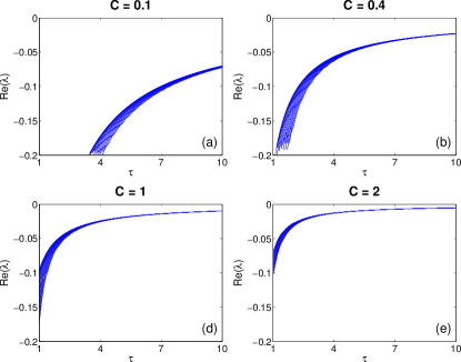
Figure 7: Real parts Re($\lambda$) of the eigenvalues of the fixed point vs. time delay $\tau$ for $a\!=\!1.05$, $\epsilon=0.01$, and (a) C=0.1, (b) C=0.4, (c) C=1, (d) C=2.

As can be seen in Fig. 7 the real parts of all eigenvalues are negative throughout, i. e., the fixed point of the coupled system remains stable for all $C$. This can be shown analytically for $a>1$ by demonstrating that no delay-induced Hopf bifurcation can occur. Substituting the ansatz $\lambda=i\omega$ into Eq. (14) and separating into real and imaginary parts yields for the imaginary part

$$\xi=\pm C\cos(\omega\tau)$$ (15)

This equation has no solution for $a>1$ since $|\xi|=a^{2}-1+C>C$, which proves that a Hopf bifurcation cannot occur.

IV.2 Delay-induced antiphase oscillations

Delay-induced oscillations in excitable systems are inherently different from noise-induced oscillations. The noise term continuously kicks the subsystems out of their respective rest states, and thus induces sustained oscillations. Instantaneous coupling without delay then produces synchronization effects between the individual oscillators HAU06 ; HOE07 ; HOE08 . For delayed coupling the case is entirely different. Here the impulse of one neuron triggers the other neuron to emit a spike, which in turn, after some delay, triggers the first neuron to emit a spike. Hence self-sustained periodic oscillations can be induced without the presence of noise (Fig. 8). It is evident that the oscillations of the two neurons have a phase lag of $\pi$. The period of the oscillations is given by $T=2(\tau+\delta)$ with a small quantity $\delta>0$.

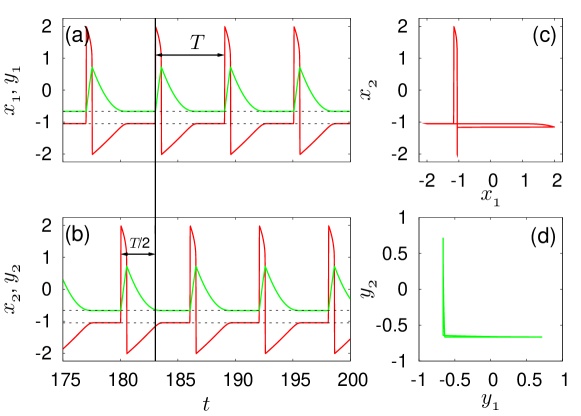
Figure 8: Delay-induced oscillations. (a), (b): Time series of both subsystems (red solid lines: activator $x_{i}$, green solid lines: inhibitor $y_{i}$; black dashed lines: fixed point values of activator and inhibitor). (c), (d): Phase portraits of activators (c) and inhibitors (d). Parameters: $a\!=\!1.05$, $\epsilon=0.01$, $C=0.5$, $\tau=3$.

In order to understand this additional phase-shift $\delta$, we shall now consider in detail the different stages of the oscillation as marked in Fig. 2. Due to the small value of $\epsilon\ll 1$ there is a distinct timescale separation between the fast activators and the slow inhibitors, and a single FitzHugh-Nagumo system performs a fast horizontal transition $A\to B$, then travels slowly approximately along the right stable branch of the $x_{1}$ nullcline $B\to C$ (firing), then jumps back fast to $D$, and returns slowly to the rest state $A$ approximately along the left stable branch of the $x_{1}$ nullcline (refractory phase). If $a$ is close to unity, these four points are approximately given by $A=(-a,-a+\frac{a_{1}^{3}}{3})$, $B=(2,-\frac{2}{3})$, $C=(1,\frac{2}{3})$, $D=(-2,\frac{2}{3})$. A rough estimate for $A^{\prime}$ is $(a-2,-a+\frac{a_{1}^{3}}{3})$. The two slow phases $B\to C$ and $D\to A$ can be approximated by $y_{1}\approx x_{1}-\frac{x_{1}^{3}}{3}$ and hence $\dot{y}_{1}\approx\dot{x}_{1}(1-x_{1}^{2})=x_{1}+a$ which gives

$$\dot{x}_{1} = \frac{x_{1}+a}{1-x_{1}^{2}}$$ (16)

which can be solved analytically, describing the firing phase (+) and the refractory phase (-):

$$\int_{\pm 2}^{x}dx_{1}\frac{1-x_{1}^{2}}{x_{1}+a}=(a^{2}-1)\ln\frac{a\pm 2}{a+x}-a(\pm 2-x)+2-\frac{x^{2}}{2}=t.$$ (17)

Integrating from $B$ to $C$ gives the firing time

$$T_{f}=\int_{2}^{1}dx_{1}\frac{1-x_{1}^{2}}{x_{1}+a}=(a^{2}-1)\ln\frac{a+2}{a+1}-a+\frac{3}{2}.$$ (18)

For $\epsilon=0.01$, $a=1.05$ the analytical solution is in good agreement with the numerical solution in Fig. 2(b), including the firing time $T_{f}=0.482$ (analytical approximation: $0.491$).

For a rough estimate, in the following we shall approximate the spike by a rectangular pulse

$$x_{1}(t)\approx\left\{\begin{array}[]{ll}2&\mbox{if }\,\,t<T_{f}\\ -a&\mbox{if }\,\,t\geq T_{f}\end{array}\right.$$ (19)

If the first subsystem is in the rest state, and a spike of the second subsystem arrives at $t=0$ (after the propagation delay $\tau$), we can approximate the initial dynamic response by linearizing $x_{1},y_{1}$ around the fixed point $(x_{1}^{*},y_{1}^{*})$ and approximating the feedback by a constant impulse during the firing time $T_{f}$. The fast dynamic response along the $x_{1}$ direction is then given by

$$\epsilon\delta\dot{x}_{1} = \xi\delta x_{1}+2C$$ (20)

with $\xi<0$. This inhomogeneous linear differential equation can be solved with the initial condition $x_{1}(0)=-a$:

$$x_{1}(t) = -a+\frac{2C}{|\xi|}(1-e^{-\frac{|\xi|}{\epsilon}t})$$ (21)

Note that this equation is not valid for large $t$ since (i) the linearization breaks down, and (ii) the pulse duration $T_{f}$ is exceeded. For small $t$ Eq.(21) can be expanded as

$$x_{1}(t) = -a+\frac{2C}{\epsilon}t$$ (22)

which is equivalent to neglecting the upstream flow field $-|\xi|\delta x_{1}$ in Eq.(20) near the stable fixed point $A$ compared to the pulling force $2C$ of the remote spike which tries to excite the system towards $B$. Once the system has crossed the middle branch of the $x_{1}$ nullisocline at $A^{\prime}$, the intrinsic flow field accelerates the trajectory fast towards $B$, initiating the firing state. Therefore there is a turn-on delay $\delta$, given by the time the trajectory takes from $A$ to $A^{\prime}$, i.e. $x_{1}(\delta)\approx a-2$, according to Eq.(22):

$$\delta = (a-1)\frac{\epsilon}{C}$$ (23)

Since the finite rise time of the impulse has been neglected in our estimate, the exact solution $\delta$ is slightly larger and does not vanish at $a=1$.

With increasing $a$ the distance $A-A^{\prime}$ increases, and so does $\delta$. The small additional phase shift $\delta$ between the spike $x_{1}(t)$ and the delayed pulse $x_{2}(t-\tau)$ results in a non-vanishing coupling term at the beginning and at the end of the spike $x_{1}(t)$. It is the reason (i) that the spike is initiated, and (ii) that it is terminated slightly before the turning point of the $x_{1}$ nullcline. The latter effect becomes more pronounced if $a$ is increased or $\tau$ is decreased (Fig. 9). Both lead to a shift of the initial starting point of the spike emission on the left branch of the nullcline towards $D$, and hence to a longer distance up to the middle branch of the nullcline which has to be overcome by the impulse $x_{2}$, hence to a larger turn-on delay $\delta$, and therefore to an earlier termination of the spike $x_{1}$. This explains that the firing phase is shortened, and the limit cycle loop is narrowed from both sides with increasing $a$ or decreasing $\tau$, see Fig. 9. In the case of $a=1.05$ and $\tau=3$ (Fig. 9 (a)), the delay time is large enough for the two subsystems to nearly approach the fixed point $A$ before being perturbed again by the remote signal. If the delay time becomes much smaller, e. g., for $\tau=0.8$ (Fig. 9 (b)), the excitatory spike of the other subsystem arrives while the first system is still in the refractory phase, so that it cannot complete the return $D\to A$ to the fixed point. In this case, $a$ in Eq.(23) has to be substituted by a larger value $\tilde{a}$ with $a<\tilde{a}<1.7$ in order to get a better estimate of $\delta$. Note that without the phase-shift $\delta$ the coupling term $C[x_{2}(t-\tau)-x_{1}(t)]$ would always vanish in the $2\tau$-periodic state.

Next, we shall investigate conditions upon the coupling parameters $C$ and $\tau$ allowing for limit cycle oscillations. On one hand, if $\tau$ becomes smaller than some $\tau_{min}$, the impulse from the excitatory neuron arrives too early to trigger a spike, since the system is still early in its refractory phase. On the other hand, if $C$ becomes too small, the coupling force of the excitatory neuron is too weak to excite the system above its threshold and pull it far enough towards $B$.

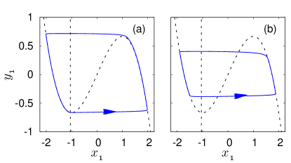
Figure 9: Phase portraits of delay-coupled excitable system $(x_{1},y_{1})$ for different delay times $\tau$ (trajectories: solid blue, nullclines: dashed black). (a) $\tau\!=\!3$ ($\delta=0.009$), (b) $\tau\!=\!0.8$ ($\delta=0.015$). Other parameters: $a\!=\!1.05$, $\epsilon\!=\!0.01$, $C\!=\!0.5$.

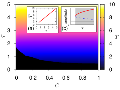
Figure 10: Regime of oscillations in the $(\tau,C)$ parameter plane for initial conditions corresponding to single-pulse-excitation in one system. The oscillation period $T$ is color coded. The transition between black and color marks the bifurcation line. Inset (a) shows the oscillation period vs. $\tau$ in a cut at $C=0.8$. Inset (b): schematic plot of the saddle-node bifurcation of a stable (red solid line) and unstable (blue dashed) limit cycle. The maximal oscillation amplitude is plotted vs. the delay time $\tau$ and the stable fixed point is plotted as a solid black line. The grey background marks the bistable region. Parameters: $a=1.05$, $\epsilon=0.01$.

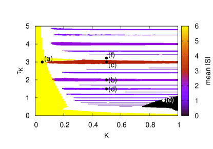
Figure 11: Influence of delayed self-feedback upon coupled oscillations. The mean interspike interval (ISI) is color coded in the control parameter plane of the self-feedback gain $K$ and delay $\tau_{K}$. White areas mark regimes of irregular oscillations where the ISI variance becomes large ($>0.01$). Time series corresponding to points (a)-(f) are shown in Fig. 12. Other parameters: $a=1.3$, $\epsilon=0.01$, $C=0.5$, $\tau=3$.

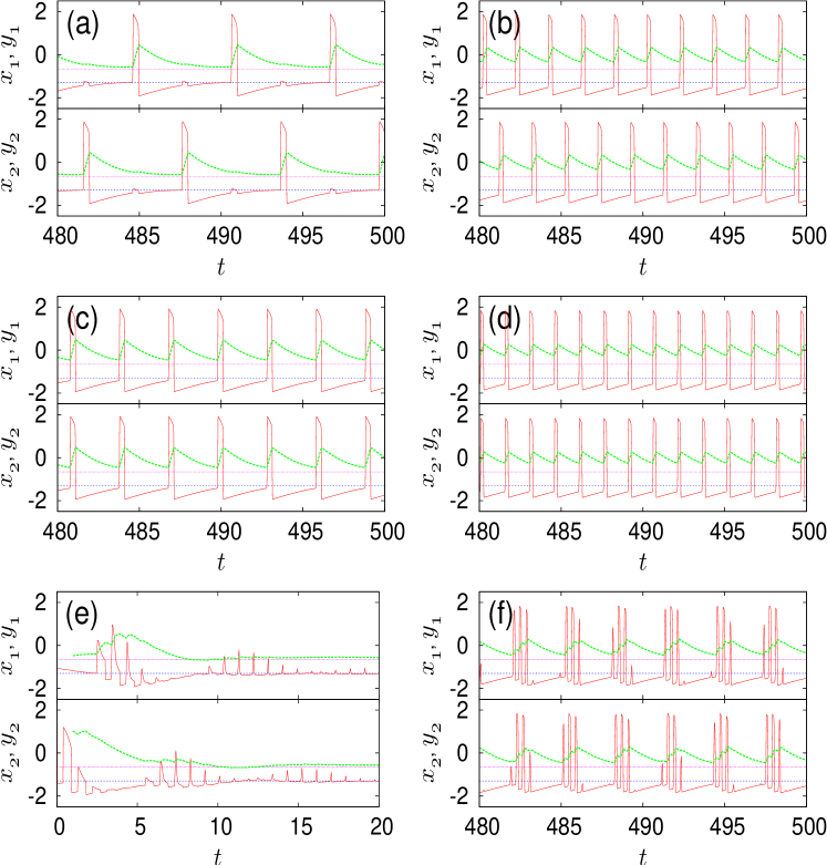
Figure 12: Different modes of oscillation corresponding to different self-feedback parameters $K$, $\tau$ (red solid lines: activators $x_{i}(t)$, green solid lines: inhibitors $y_{i}(t)$). (a), (b): Antiphase oscillations for (a) $K=0.05,\tau_{K}=3$ (period $T=6$) and (b) $K=0.5,\tau_{K}=2$ ($T=2$); (c), (d): In-phase oscillations for (c) $K=0.5,\tau_{K}=3$ (period $T=3$) and (d) $K=0.5,\tau_{K}=1.5$ ($T=1.5$); (e): Oscillator death for $K=0.9,\tau_{K}=0.9$; (f): Bursting pattern for $K=0.5,\tau_{K}=3.2$. Other parameters: $a=1.3$, $\epsilon=0.01$, $C=0.5,\tau=3$.

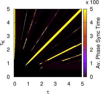
Figure 13: Average phase synchronization time (color coded) in the control parameter plane of coupling delay $\tau$ and self-feedback delay $\tau_{K}$. Other parameters: $a=1.3$, $\epsilon=0.01$, $C=0.5$, $K=0.5$.

In Fig. 10 the regime of oscillations is shown in the parameter plane of the coupling strength $C$ and coupling delay $\tau$. The oscillation period is color coded. The boundary of this colored region is given by the minimum coupling delay $\tau_{min}$ as a function of $C$. For large coupling strength, $\tau_{min}$ is almost independent of $C$; with decreasing $C$ it sharply increases, and at some small minimum $C$ no oscillations exist at all. At the boundary, the oscillation sets in with finite frequency and amplitude as can be seen in the insets of Fig. 10 which show a cut of the parameter plane at $C=0.8$. The oscillation period increases linearly with $\tau$. The mechanism that generates the oscillation is a saddle-node bifurcation of limit cycles (see inset (b) of Fig. 10), creating a pair of a stable and an unstable limit cycle. The unstable limit cycle separates the two attractor basins of the stable limit cycle and the stable fixed point.

V Delayed self-feedback and delayed coupling

In this section we consider the simultaneous action of delayed coupling and delayed self-feedback. Here we choose to apply the self-feedback term symmetrically to both activator equations, but other feedback schemes are also possible.

$$\epsilon_{1}\dot{x}_{1} = x_{1}-\frac{x_{1}^{3}}{3}-y_{1}+C[x_{2}(t-\tau)-x_{1}(t)]+K[x_{1}(t-\tau_{K})-x_{1}(t)]$$

$$\dot{y}_{1} = x_{1}+a$$

$$\epsilon_{2}\dot{x}_{2} = x_{2}-\frac{x_{2}^{3}}{3}-y_{2}+C[x_{1}(t-\tau)-x_{2}(t)]+K[x_{2}(t-\tau_{K})-x_{2}(t)]$$

$$\dot{y}_{2} = x_{2}+a$$ (24)

By a linear stability analysis similar to Sect. 4.1 it can be shown that the fixed point remains stable for all values of $K$ and $\tau_{K}$ in case of $a>1$, as without self-feedback. Redefining $\xi=1-a^{2}-C-K$, one obtains the factorized characteristic equation

$$1-\xi\lambda+\epsilon\lambda^{2}=\lambda Ke^{-\lambda\tau_{K}}\pm\lambda Ce^{-\lambda\tau}$$ (25)

Substituting the Hopf condition $\lambda=i\omega$ and separating into real and imaginary parts yields for the imaginary part

$$-\xi=K\cos(\omega\tau_{K})\pm C\cos(\omega\tau)$$ (26)

This equation has no solution for $a>1$ since $|\xi|=a^{2}-1+C+K>C+K$.

The adopted form of control allows for the synchronization of the two cells not only for identical values of $\tau$ and $\tau_{K}$, but generates an intricate pattern of synchronization islands or stripes in the control parameter plane (Fig. 11) corresponding to single-spike in-phase and antiphase oscillations with constant interspike intervals, see also Fig. 12(a)-(d). Further, for adequately chosen parameter sets of coupling and self-feedback control, we observe effects such as bursting patterns Fig. 12(f) and oscillator death Fig. 12(e). In addition to these effects, there exists a control parameter regime in which the self-feedback has no effect on the oscillation periods (shaded yellow).

Fig. 11 shows the control parameter plane for coupling parameters of the uncontrolled system in the oscillatory regime ($C=0.5$ and $\tau=3$). We observere three principal regimes: (i) Control has no effect on the oscillation period (yellow), although the form of the stable limit cycle is slightly altered (Fig. 12(a)). (ii) Islands of in-phase and antiphase synchronization (color coded, see Fig. 12 (b)-(d)). (iii) Oscillator death (black) Fig.  12 (e)).

Fig. 13 shows the average phase synchronization time as a function of the coupling delay $\tau$ and self-feedback delay $\tau_{K}$ for fixed $K=0.5$. The bright straight rays at rational $\tau_{K}/\tau$ indicate long intervals during which both subsystems remain synchronized. A particularly long average synchronization time is found if the two delay-times are equal.

VI Conclusion

Our analysis has focussed on a model of two coupled neurons, which may be viewed as a network motif for larger neural networks. We have shown that delayed feedback from other neurons or self-feedback from the same neuron can crucially affect the dynamics of coupled neurons. In case of noise-induced oscillations in instantaneously coupled neural systems, time-delayed self-feedback can enhance or suppress stochastic synchronization, depending upon the delay time. This offers promising perspectives with respect to potential therapies of pathological neural synchrony as occurring, for example, in Parkinson’s disease. It suggests that by carefully choosing the delay time, feedback control applied locally to a neural sub-population can suppress the global synchronization of the neurons.

In case of delay-coupled neurons without driving noise sources, the propagation delay of the spikes fed back from other neurons can induce periodic oscillations for sufficiently large coupling strength and delay times. Bistability of a fixed point and limit cycle oscillations occur even though the single excitable element displays only a stable fixed point. The two neurons oscillate with a phase lag of $\pi$. If self-feedback is applied additionally, for example by axonal reflections (Fig. 1 (a)) in networks of electrically coupled pyramidal cells SCH01e , synchronous zero-lag oscillations can be induced in some ranges of the control parameters, while in other regimes antiphase oscillations or oscillator death as well as more complex bursting patterns can be generated.

VII Acknowledgements

This work was supported by DFG in the framework of Sfb 555. The authors would like to thank S. Brandstetter, V. Flunkert, A. Panchuk, and F. Schneider for fruitful discussions, and Roger Traub for helpfull comments on gap junction coupling.

References

- (1) Handbook of Chaos Control, edited by E. Schöll and H. G. Schuster (Wiley-VCH, Weinheim, 2008), second completely revised and enlarged edition.
- (2) H. Haken, Brain Dynamics: Synchronization and Activity Patterns in Pulse-Coupled Neural Nets with Delays and Noise (Springer Verlag GmbH, Berlin, 2006).
- (3) H. R. Wilson, Spikes, Decisions, and Actions: The Dynamical Foundations of Neuroscience (Oxford University Press, Oxford, 1999).
- (4) W. Gerstner and W. Kistler, Spiking neuron models (Cambridge University Press, Cambridge, 2002).
- (5) S. J. Schiff, K. Jerger, D. H. Duong, T. Chang, M. L. Spano, and W. L. Ditto, Nature (London) 370, 615 (1994).
- (6) M. G. Rosenblum and A. Pikovsky, Phys. Rev. Lett. 92, 114102 (2004).
- (7) O. V. Popovych, C. Hauptmann, and P. A. Tass, Phys. Rev. Lett. 94, 164102 (2005).
- (8) E. Ott, C. Grebogi, and J. A. Yorke, Phys. Rev. Lett. 64, 1196 (1990).
- (9) K. Pyragas, Phys. Lett. A 170, 421 (1992).
- (10) J. E. S. Socolar, D. W. Sukow, and D. J. Gauthier, Phys. Rev. E 50, 3245 (1994).
- (11) M. Gassel, E. Glatt, and F. Kaiser, Fluct. Noise Lett. 7, L225 (2007).
- (12) M. Gassel, E. Glatt, and F. Kaiser, Phys. Rev. E 77, 066220 (2008).
- (13) M. A. Dahlem, F. M. Schneider, and E. Schöll, Chaos 18, 026110 (2008).
- (14) D. Schmitz, S. Schuchmann, A. Fisahn, A. Draguhn, E. H. Buhl, E. Petrasch-Parwez, R. Dermietzel, U. Heinemann, and R. D. Traub, Neuron 31, 831 (2001).
- (15) J. G. Jefferys and H. L. Haas, Nature 300, 448 (1982).
- (16) R. D. Traub, J. G. Jefferys, R. Miles, M. A. Whittington, and K. Tóth, J. Physiol. (Lond.) 48, 79 (1994).
- (17) R. D. Traub, D. Schmitz, J. G. Jefferys, and A. Draguhn, Neuroscience 92, 407 (1999).
- (18) H. R. Wilson and J. D. Cowan, Biophysical journal 12, 1 (1972).
- (19) A. Destexhe, D. Contreras, T. J. Sejnowski, and M. Steriade, J. Neurophysiol. 72, 803 (1994).
- (20) C. Zhou, L. Zemanova, G. Zamora, C. C. Hilgetag, and J. Kurths, Phys. Rev. Lett. 97, 238103 (2006).
- (21) R. FitzHugh, Biophys. J. 1, 445 (1961).
- (22) J. Nagumo, S. Arimoto, and S. Yoshizawa., Proc. IRE 50, 2061 (1962).
- (23) B. Lindner, J. García-Ojalvo, A. Neiman, and L. Schimansky-Geier, Phys. Rep. 392, 321 (2004).
- (24) D. T. J. Liley and J. J. Wright, Network: Computation in Neural Systems V5, 175 (1994).
- (25) R. D. Pinto, P. Varona, A. R. Volkovskii, A. Szücs, H. D. I. Abarbanel, and M. I. Rabinovich, Phys. Rev. E 62, 2644 (2000).
- (26) F. F. De-Miguel, M. Vargas-Caballero, and E. García-Pérez, J. Exp. Biol. 204, 3241 (2001).
- (27) N. Buric and D. Todorovic, Phys. Rev. E 67, 066222 (2003).
- (28) V. Hadamschek, Brain stimulation techniques via nonlinear delayed neurofeedback based on MEG inverse methods, PhD Thesis, TU Berlin (2006).
- (29) P. Tass, Phys. Rev. E 66, 036226 (2002).
- (30) B. Hauschildt, N. B. Janson, A. G. Balanov, and E. Schöll, Phys. Rev. E 74, 051906 (2006).
- (31) P. Hövel, M. A. Dahlem, and E. Schöll, in Proc. 19th Internat. Conf. on Noise and Fluctuations (ICNF-2007) (American Institute of Physics, College Park, Maryland 20740-3843, 2007).
- (32) M. G. Rosenblum, A. Pikovsky, and J. Kurths, Synchronization – A universal concept in nonlinear sciences (Cambridge University Press, Cambridge, 2001).
- (33) P. Hövel, M. A. Dahlem, and E. Schöll, submitted (2008).
- (34) N. B. Janson, A. G. Balanov, and E. Schöll, Phys. Rev. Lett. 93, 010601 (2004).
- (35) A. G. Balanov, N. B. Janson, and E. Schöll, Physica D 199, 1 (2004).
- (36) T. Prager, H. P. Lerch, L. Schimansky-Geier, and E. Schöll, J. Phys. A 40, 11045 (2007).
- (37) E. Schöll, A. G. Balanov, N. B. Janson, and A. Neiman, Stoch. Dyn. 5, 281 (2005).
- (38) J. Pomplun, A. Amann, and E. Schöll, Europhys. Lett. 71, 366 (2005).
- (39) A. Pototsky and N. B. Janson, Phys. Rev. E 76, 056208 (2007).
- (40) V. Flunkert and E. Schöll, Phys. Rev. E 76, 066202 (2007).
- (41) J. Hizanidis, A. G. Balanov, A. Amann, and E. Schöll, Phys. Rev. Lett. 96, 244104 (2006).
- (42) J. Hizanidis and E. Schöll, phys. stat. sol. (c) 5, 207 (2008).
- (43) G. Stegemann, A. G. Balanov, and E. Schöll, Phys. Rev. E 73, 016203 (2006).
- (44) A. G. Balanov, V. Beato, N. B. Janson, H. Engel, and E. Schöll, Phys. Rev. E 74, 016214 (2006).
- (45) J. Pomplun, A. G. Balanov, and E. Schöll, Phys. Rev. E 75, 040101(R) (2007).
- (46) E. Schöll, N. Majer, and G. Stegemann, phys. stat. sol. (c) 5, 194 (2008).