Matter-wave cavity gravimeter

Abstract

We propose a gravimeter based on a matter-wave resonant cavity loaded with a Bose-Einstein condensate and closed with a sequence of periodic Raman pulses. The gravimeter sensitivity increases quickly with the number of cycles experienced by the condensate inside the cavity. The matter wave is refocused thanks to a spherical wave-front of the Raman pulses. This provides a transverse confinement of the condensate which is discussed in terms of a stability analysis. We develop the analogy of this device with a resonator in momentum space for matter waves.

The realization of gravimeters loaded with cold atomic clouds has drastically increased the accuracy of the measurement of gravitational acceleration to a few parts per billion Peters et al. (1999, 2001). The recent obtention of quasi-continuous atom lasers now opens new perspectives for gravito-inertial sensors with the possibility to load these devices with a fully coherent and collimated matter source instead of the incoherent cold atomic samples used so far. In this paper we investigate a gravimeter based on a resonant matter-wave cavity loaded with a Bose-Einstein condensate. The condensate is stabilized in momentum space thanks to a sequence of periodic “mirror pulses” consisting in velocity-sensitive double Raman $\pi$-pulses. Between the pulses, the optical potential is shut off and the condensate experiences a pure free fall. Other measurements of the acceleration of gravity have been proposed, based on the Bloch oscillations of an atomic cloud in a standing light wave Cladé et al. (2005); Bordé et al. (1987) or on the bouncing of a cloud on an evanescent-wave optical cavity Wallis et al. (1992); Aminoff et al. (1993). In our setup, we can minimize parasitic diffusions processes Landragin et al. (1996) which may kick atoms out of the cavity and thus limit the lifetime $T_{cav}$. The expansion of the atomic cloud, whose size quickly exceeds the diameter of the mirror, usually limits the number of bounces in the cavity Aminoff et al. (1993). As in Wallis et al. (1992); Aminoff et al. (1993), we circumvent this problem by using a “curved mirror” which refocuses periodically the condensate. This gives a very promising sensitivity for the proposed gravimeter, which increases as $T_{cav}^{3/2}$ with the atom interrogation time $T_{cav}$ as in standard atom gravimeters Peters et al. (1999).

I Determination of the acceleration of gravity: principle of the measurement

Following up our approach in Impens et al. (2006), we present in this section a first simple description of the proposed matter-wave cavity and give a heuristic analysis of its performance as a gravimeter.

I.1 Principle of the experiment

The principle is to levitate a free falling atomic sample by providing a controllable acceleration mediated by a coherent atom-light interaction. Radiation pressure could provide levitation, but the resulting force is not precisely tunable if tied to incoherent spontaneous emission processes. A better choice to provide this acceleration is thus a series of vertical Raman pulses. Indeed these pulses impart coherently a very well defined momentum to a collection of atoms Weitz et al. (1994). A sequence of Raman pulses of identical effective wave vector $\mathbf{k}$ interspaced with a duration $T$ gives an acceleration to an atomic cloud which is monitored by the choice of $T$. Levitation occurs when the sequence of vertical Raman pulses compensates, on average, the action of gravity. This stabilization is obtained thanks to a fine-tuning of the period between two pulses: after a fixed time, one observes a resonance in the number of atoms kept in the cavity for the adequate period $T_{0}$. The atomic cloud is then well stabilized, and the average Raman acceleration equals the gravitational acceleration. Knowing the period $T_{0}$, one can infer the corresponding Raman acceleration and thus the gravity acceleration $g$. The ratio $\hbar k/m$ can be simultaneously determined using the resonance condition of the Raman mirrors.

I.2 Description of the cavity

As displayed in Fig.1, the atomic sample, initially at rest in the lower state $a$, is dropped. After a free fall of duration $T/2$, during which the sample acquires a momentum $gT/2$, we shine a first Raman $\pi$ pulse of $2$ counterpropagating lasers with respective wave vectors $\mathbf{k_{down}}=\mathbf{k_{1}}$ and $\mathbf{k_{up}}=\mathbf{k_{2}}$ and respective frequencies $\omega_{down}=\omega_{1}$ and $\omega_{up}=\omega_{2}$. This brings the atom from the internal state $a$ to an internal state $b$ with a momentum transfer $2\hbar k=k_{2}-k_{1}$. Then we shine a second Raman $\pi$ pulse with $\mathbf{k_{down}}=\mathbf{k_{4}}$ and $\mathbf{k_{up}}=\mathbf{k_{3}}$, with respective frequencies $\omega_{down}=\omega_{4}$ and $\omega_{up}=\omega_{3}$ $(\omega_{3}-\omega_{4}\sim\omega_{2}-\omega_{1})$. This pulse brings the atomic internal state back to state a with an additional momentum transfer $2\hbar k$. If the two successive pulses are sufficiently close, this sequence acts as a single coherent “mirror pulse” which keeps the same internal state a and modifies the atomic momentum by $4\hbar k$. In particular, if the initial momentum is $-2\hbar k$, the mirror simply inverts the velocity. This “mirror pulse” is velocity-sensitive: it reflects only the atoms whose vertical momentum belong to a tiny interval around a specific value $p_{0}$. Thus, in order to bounce several times, the atoms should have the same momentum $p_{0}$ immediately before each “mirror pulse”. This implies a resonance condition (1) on the period between two pulses. The adequate momentum $p_{0}$ is set by the energy conservation during the pulse and fulfills the resonance condition (I.3). As depicted in Fig. 2, if the resonance condition (1) is satisfied, the sample will have a periodic trajectory in the momentum space. It is this periodicity of the atomic momentum for an adequate time-spacing $T_{0}$ of two successive “mirror pulses” which yields the picture of a matter-wave cavity in momentum space. Fig. 3 represents an energy-momentum diagram of the atomic sample during a cavity cycle.

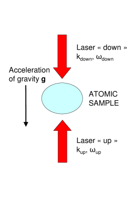
Figure 1: Setup description.

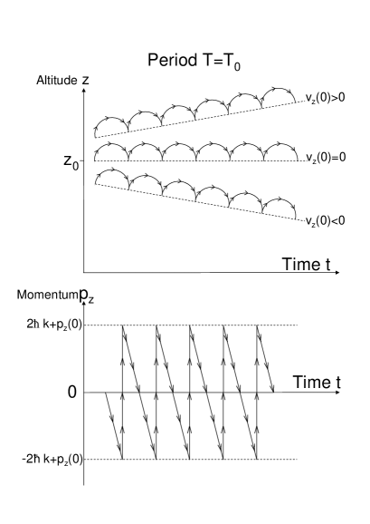
Figure 2: Altitude and momentum of the atom sample as a function of time for the resonant period $T=T_{0}$ and for different initial velocities. The atom cloud always undergoes a periodic motion in momentum space even with a nonzero initial velocity. The figure illustrates three different cases of stable cavity in momentum space.

Figure 3: Energy-momentum diagram of the condensate. $z_{0}$ represents the height from which atoms are dropped.

I.3 Resonance Conditions

For the resonant period $T_{0}$, the momentum kick imparted during each “mirror pulse” is equal to the momentum acquired through the free fall between two such pulses:

$$T_{0}=\frac{4\hbar k}{mg}$$ (1)

If the period $T$ differs from $T_{0}$, the atomic cloud takes an acceleration $a=4\hbar k/m\left(1/T-1/T_{0}\right)$. The average speed resulting from this acceleration drifts the momentum of the atoms from the optimum value $\mathbf{p_{0}}=-2\hbar k\mathbf{u_{z}}$ satisfying the Bragg condition (I.3) associated with elastic energy conservation. This drives the atoms progressively out of resonance and a part of the cloud will not be reflected by the “mirror pulses”. When $T$ differs from $T_{0}$, we thus observe a drift in position and momentum as well as a leakage of the condensate. It should be noted that if $T=T_{0}$, a non-zero initial velocity does not reduce fundamentally the number of bounces of an atomic sample (Fig. 2). Indeed, only the periodicity of the momentum space trajectory matters, and provided that one adjusts the Raman detuning to account for the shift in the momentum $p_{0}$, the sample can still be reflected several times. The atomic sample merely drifts with a constant average vertical velocity, the only limitation being then the finite size of the experiment. Thanks to this flexibility in the initial velocity, the resonance observed is robust to an imperfect timing of the trap shutdown.

Bragg resonance conditions express the energy conservation during the pulses:

$$\omega_{1}+\omega_{b}+\delta_{AC}+\frac{(\textbf{p}+2\hbar\textbf{k})^{2}}{2m\hbar}=\omega_{2}+\omega_{a}+\frac{\textbf{p}^{2}}{2m\hbar}$$

$$\omega_{4}+\omega_{a}+\frac{(\textbf{p}+4\hbar\mathbf{k})^{2}}{2m\hbar}=\omega_{3}+\omega_{b}+\delta_{AC}+\frac{(\textbf{p}+2\hbar\mathbf{k})^{2}}{2m\hbar}$$ (2)

p is the matter-wave average momentum immediately before the first Raman pulse, and $\delta_{AC}$ is the light shift. Thanks to this second set of conditions, which directly impacts the reflection coefficient, the “mirror pulses” act directly as the probe of the resonant time-spacing $T_{0}$ expressed in (1). When the atomic sample is dropped without initial speed, for a nearly resonant period $T\simeq T_{0}$, the first pulse brings the sample at rest, so that both pulses play a symmetric role. If one does the replacements $\omega_{1}\rightarrow\omega_{3}$ and $\omega_{2}\rightarrow\omega_{4}$, the mismatch in the two Bragg conditions is then equal in absolute value, yielding identical reflection coefficients for both pulses. One can then consider that the two Bragg conditions merge into a single one. We assume from now on that the atomic cloud has no initial velocity , but the extension to the general case is straightforward.
The two conditions (1) and (I.3) must be satisfied to ensure the resonance of the matter-wave cavity. Nonetheless, condition (1) on the period is much more critical than the Bragg condition (I.3). Indeed, a slight shift in the period $T$ from its optimum value $T_{0}$ implies for the condensate an upward or downward acceleration. The increasing speed acquired by the atoms will generate, through Doppler shifting, a greater violation of the Bragg resonance condition and thus greater losses at each “mirror pulse”. Conversely, a mismatch in the detuning $\omega_{2}-\omega_{1}$ with the adjustment $T=T_{0}$ will only induce constant losses at each cycle. The observation of a resonance in the number of atoms, when one scans the period between two Raman pulses, is thus very sharp and robust to an imperfect adjustment of the Raman detuning. Consistently, we choose to determine the acceleration of gravity $g$ through condition (1). Fig. 4 sketches the number of atoms in the cavity as a function of the period $T$ after different numbers of cycles with a detuning matching perfectly condition (I.3). We observe that the resonance in $T$ becomes sharper as the number of cycles increases.

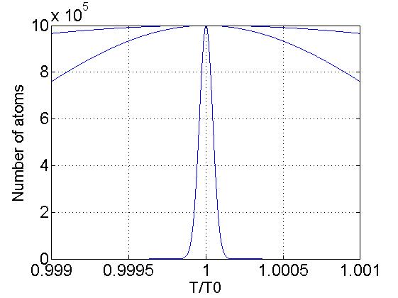
Figure 4: Number of atoms in the cavity after 1,10,50 cycles as a function of the ratio $T/T_{0}$ $(T_{0}\simeq 3.8\>\mbox{ms})$. We took $\Omega_{0}=2\pi\times 5\times 10^{3}\>\mbox{Hz}$. The number of atoms initially present in the cavity was fixed to be $N=10^{6}$.

I.4 Expected Sensitivity

Let us derive the resonance figure associated with the period $T$. We characterize the mismatch in the Bragg condition by an “off-Braggness” parameter $y(\mathbf{p})$ function of the average momentum of the atoms Bordé (1997):

$$y(\mathbf{p})=\frac{1}{2\Omega_{0}}[\hbar\mathbf{k}^{2}/2m+2\mathbf{p}\cdot\mathbf{k}/m-(\omega_{1}-\omega_{2}-\omega_{ba}-\delta_{AC})]$$ (3)

where $\Omega_{0}$ the effective Rabi frequency of the Raman pulse and $\mathbf{p}$ the momentum immediately before the first pulse.. The Raman detuning is adjusted to be resonant if $\mathbf{p}=p_{0}\mathbf{u_{z}}=-2\hbar k\mathbf{u_{z}}$, so we adjust the detuning to match $y(-2\hbar k\mathbf{u_{z}})=0$:

$$y(\mathbf{p})=\frac{(p_{z}+2\hbar k)k}{2m\Omega_{0}}=\frac{(p_{z}+mgT_{0}/2)k}{2m\Omega_{0}}$$ (4)

In the remainder of this section, we focus on the vertical component of momentum which we note $p$ to alleviate the notations. Because of the mismatch in the Bragg condition, only a fraction $\rho(p)$ of the atomic cloud will then be transferred during the first Raman pulse:

$$\rho(p)=\frac{\sin^{2}\left(\frac{\pi}{2}\sqrt{1+y(p)^{2}}\right)}{1+y(p)^{2}}$$ (5)

For the second Raman pulse, the mismatch is equal in value and opposite in sign, so the same fraction of atoms undergoes the second transition. The reflection coefficient of the “mirror pulse” is then simply the product of these values:

$$R(p)=\frac{\sin^{4}\left(\frac{\pi}{2}\sqrt{1+y(p)^{2}}\right)}{(1+y(p)^{2})^{2}}$$ (6)

The part of the cloud which is not reflected will simply go on a free fall and have an off-Braggness parameter of $y(p-mgT)$ for the next “mirror pulse”. We will adopt experimental parameters such that $y(mgT_{0})\gg 1$, so that non-reflected atoms are insensitive to subsequent Raman transitions and can be considered as expelled from the cavity.

The average momentum acquired by the atomic cloud results from a competition between the gravitational acceleration and the kicks of the “mirror pulses”. Given a period $T$ for the sequence, the average vertical momentum of the cloud immediately before the n-th “mirror pulse” is simply:

$$p_{n} = -mgT/2+(n-1)\times mg(T_{0}-T)$$ (7)

The remaining fraction of the cloud after $n$ cycles is thus:

$$R(T)=R(p_{1})...R(p_{n})$$ (8)

We expand this expression in Appendix A for nearly resonant pulses. We have assumed that a relative variation $\epsilon$ of the condensate population can be tracked experimentally. This computation shows that the error in the determination of the gravity acceleration can be less than:

$$\frac{|\Delta{g}|}{g}\leq\sqrt{\frac{3}{8}}\frac{1}{\hbar k^{2}}\left(\frac{\Omega_{0}\sqrt{-\log(1-\epsilon)}}{n^{3/2}}\right)+|\frac{\Delta v_{r}}{v_{r}}|$$ (9)

where $v_{r}=\hbar k/m$ is a recoil velocity which can be measured independently or, as stated before, directly from resonance condition (I.3) Coq et al. (2001). This velocity has been determined with an accuracy as good as a few $10^{-9}$ for Cs Weiss et al. (1993); Wicht et al. (2002) and Rb atoms Battesti et al. (2004), ultimately limits the performance of our gravimeter. Fig. 5 displays the relative error in the determination of the acceleration of gravity obtained from a numerical simulation with the reflection coefficient (6). It shows a very good agreement with the analytic expression (9) after about $10$ cycles.

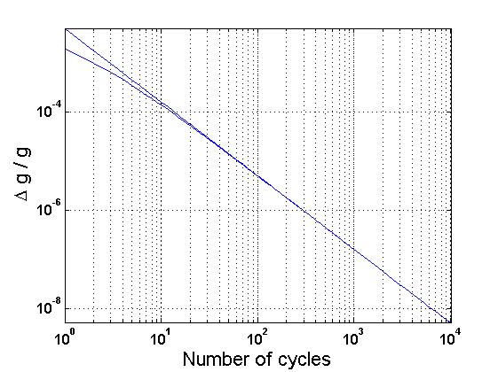
Figure 5: Error on $\Delta g/g$ as a function of the number of cycles, with Raman pulses of Rabi pulsation $\Omega_{0}=2\pi\times 5\times 10^{3}Hz$ and a detection threshold of $\epsilon=10^{-3}$. The lower curve is the actual sensitivity based on a simulation with a condensate of infinitely narrow momentum distribution. The upper curve is the analytic formula (9).

Formula (9) thus yields a sensitivity which scales as $n^{3/2}=(T_{cav}/T_{0})^{3/2}$, where $T_{cav}$ is the interrogation time of the atoms and $T_{0}$ the duration of a cycle at resonance. We thus obtain the expected improvement of the sensitivity with the atom interrogation time. This is normal since the accuracy of the measurement also increases with the selectivity of the Raman pulses. The mirror pulses should thus be as long as possible to act as efficient atom velocity probes. Ideally, each pulse should last half of the optimal period $T_{0}$. The atom sample would then fall in a continuous light field. This setup ressembles that of Cladé et al. Cladé et al. (2005), except that here the atomic sample is interacting with a travelling wave, and that in addition to condition (1) we have a double Raman condition (I.3).

In the previous description, one could in principle maintain the sample for an arbitrary long time inside the cavity provided that the two resonance conditions are fulfilled, yielding an extremely accurate measurement of the gravitational acceleration. In fact, even at resonance, systematic losses occur that limit the number of condensate cycles. Practically, one can hope to keep a significant number of atoms in the cloud up to a certain number of $n$ cycles, which reflects the sample lifetime $T_{cav}=nT_{0}$ at resonance. These losses at resonance have several origins.

First, they can result from imperfect recoil transfers due to residual fluctuations in the Raman lasers intensities. Raman impulsions can be very effective though, since these transfers have been realized with an efficiency as high as $99.5\%$.

Second, parasitic diffusions may eject atoms from the cavity. These processes, such as absorption followed by spontaneous emission, can be made arbitrarily small by using far-detuned Raman pulses. This limitation is thus essentially of technical nature.

Third, the cloud expansion can drive the atomic sample out of the Raman lasers. Indeed, if the cloud is not refocused, its transverse size exceeds quickly the diameter of the Raman lasers. The atoms would then be limited to a few cycles in the cavity. It is thus essential to involve a mechanism that stabilizes transversally the atomic cloud. We expose in Section III two ways to focus the atomic sample.

II ABCD analysis of the matter-wave cavity

In the following, we will calculate explicitly the evolution of an atom sample in our gravitational cavity using the ABCD matrix formalism Bordé (1992, 2001a, 2001b). In this section, we assume that the atom density after the initial free fall is sufficiently low to make the effect of interactions negligible during the subsequent bounces.

II.1 Description of the atomic sample

We will restrict ourselves to a Bose-Einstein condensate which, in the Hartree-Fock approximation, can be described by a macroscopic wavefunction $\Psi(\mathbf{r},t)$. After the initial free-fall, the evolution follows the linear partial differential equation:

$$i\hbar\partial_{t}|\Psi(\mathbf{r},t)\rangle=[p^{2}/2m+H_{\mbox{G}}]|\Psi(\mathbf{r},t)\rangle$$ (10)

where $H_{\mbox{G}}$ is the Hamiltonian associated with gravito-inertial effects. From the linearity of this equation, we can deduce the time evolution of any arbitrary wave function from the propagation of a complete set of functions. As explained in Appendix C, the propagation of such a basis, the Hermite-Gauss modes $H_{lmn}(\mathbf{r})$, can be extracted from the propagation of a generating Gaussian wave function Bordé (2001b):

$$\Psi_{\overrightarrow{\alpha}}(\mathbf{r})=\frac{1}{\sqrt{\mbox{det}(X_{0})}}\exp[\frac{im}{2\hbar}(\mathbf{r}-\mathbf{r_{0}})Y_{0}X_{0}^{-1}(\mathbf{r}-\mathbf{r_{0}})$$

$$+\frac{i}{\hbar}(\mathbf{r}-\mathbf{r_{0}})\cdot(\mathbf{p_{0}}-2\hbar\tilde{X_{0}^{-1}}\overrightarrow{\alpha})+\frac{1}{2}\overrightarrow{\alpha}X_{0}^{-1}X_{0}^{*}\overrightarrow{\alpha}]$$ (11)

The matrices $X_{0},Y_{0}$ and the vectors $\mathbf{r_{0}},\mathbf{p_{0}}$ correspond respectively to the position and momentum widths, to the average position and to the average momentum of the wave function. We can then restrict our derivation without any loss of generality to the propagation of (II.1). Since the Hamiltonian $H_{\mbox{G}}$ can be considered with a very good approximation to be quadratic in position and momentum, the wave-packet (II.1) follows the ABCD law for atom optics Bordé (2001a). In order to alleviate the notations, we shall omit to mention the index $\overrightarrow{\alpha}$ in the subsequent computations and denote the corresponding state $|\Psi_{\mathbf{r_{0}},\mathbf{p_{0}},X_{0},Y_{0}}\rangle$.

II.2 Initial Expansion

Before the trap shutdown, the condensate evolves under the Hamiltonian $H=p^{2}/2m+H_{G}+H_{\mbox{Trap}}$. We remove the gravitational term $H_{G}$ thanks to a unitary transform $U_{G}(t,t_{0})$:

$$|\Psi(t)\rangle=U_{G}(t,t_{0})|\Phi(t)\rangle$$ (12)

$U_{G}(t,t_{0})$ represents the evolution of a quantum state under a gravitational field. Performing this unitary transform is equivalent to study the condensate in the non-inertial free falling frame. The state $|\Phi(t)\rangle$ then evolves under the Hamiltonian $H_{FreeFall}=p^{2}/2m+H_{\mbox{Trap}}$. The condensate is taken to be initially in the strong coupling regime, so that the corresponding wave function $\Phi(\mathbf{r},t)$ follows the scaling laws established by Castin and Dum Castin and Dum (1996) for the Thomas-Fermi expansion. The initial wave function $\Phi(\mathbf{r},t_{0})$ corresponds to the Thomas-Fermi profile. We represent concisely its evolution by the unitary transform $U_{TFE}(t,t_{0})$:

$$|\Phi(t)\rangle=U_{TFE}(t,t_{0})|\Phi(t_{0})\rangle$$ (13)

It is indeed not useful at this point to explicit this transform, whose expression is given in Appendix B. We transform back to the laboratory frame at the time $t_{1}$ when we start to shine the first “mirror pulse”:

$$|\Psi(t_{1})\rangle=U_{G}(t_{1},t_{0})U_{TFE}(t_{1},t_{0})|\Phi(t_{0})\rangle$$ (14)

The resulting quantum state $|\Psi(t_{1})\rangle$ will be taken as a starting point for the subsequent oscillation of the condensate in the cavity. Its evolution is conveniently obtained by decomposition on a suitable basis of Hermite-Gauss modes $H_{lmn}(\mathbf{r})$, as explained in the preceding paragraph. The initial free fall simply determines the initial coefficients of the projection:

$$\hat{\Psi}(\mathbf{r},t_{1})=\sum_{l,m,n}c_{lmn}(t_{1})H_{lmn}(\mathbf{r})$$ (15)

II.3 Propagation of a Gaussian wave-packet in the diluted regime

The evolution of free falling atoms in a Raman pulse is non-trivial since the gravitational acceleration makes the detuning (3) time-dependent:

$$\Delta(t)=\omega_{1}-\omega_{2}-\omega_{ba}-2(\mathbf{p}-mg\>t\>\mathbf{u}_{z})\cdot\mathbf{k}/m$$

$$-2\hbar\mathbf{k}^{2}/m-\delta_{AC}$$ (16)

The behavior of a two-level atom falling into a laser wave has been solved exactly Bordé and Lämmerzahl (1995). Gravitation alters significantly the two-level atom state trajectory on the Bloch sphere when the pulse duration $\tau$ becomes of the order of:

$$\tau_{g}=\frac{1}{\sqrt{||\mathbf{k}||||\mathbf{g}||}}\simeq 10^{-4}s$$ (17)

Indeed, for this duration the off-Braggness parameter (3) changes significantly during the pulse. As seen in the previous section, in order to probe effectively the resonance condition (1), the Raman $\pi$-pulses need to be velocity-selective. This leads us to consider pulse durations on the order of the millisecond, typically longer than $\tau_{g}$. It is then necessary to compensate the time-dependent term induced by the acceleration of gravity in the detuning by an opposite frequency ramp chirping the pulse.

The simultaneous effects of gravito-inertial and electromagnetic fields can be decoupled thanks to an effective propagation scheme developped by Antoine and Bordé Bordé (2001a, b). It accounts for the electromagnetic interaction through an instantaneous diffusion matrix $\hat{S}$ and for gravito-inertial effects through a unitary transform $U_{1}(T,0)$:

$$|\Psi(T)\rangle=U_{1}(T,0)\>\hat{S}\>|\Psi(0)\rangle$$ (18)

Following this propagation method, it is sufficient to apply an effective instantaneous diffusion matrix for each “mirror pulse” and evolve the state between the pulse centers as if there was no electromagnetic field.

II.4 Action of the effective instantaneous interaction matrix $\hat{S}$

We study in this paragraph the interaction of the condensate with a quasi-plane electromagnetic wave, for which the instantaneous diffusion matrix $\hat{S}$ is known. This matrix is operator-valued, but momentum operators can be taken as complex-numbers since the considered wave function is a narrow momentum wave-packet centered around a nearly resonant momentum $\mathbf{p_{0}}$ (i.e. such that $y(p_{0})\ll 1$). In other circumstances, this interaction can give rise to fine structuring effects such as the splitting of the initial wave into several packets following different trajectories (Borrmann effect) Bordé (1997). Following the approach of the paragraph II.1, we consider a Gaussian matter-wave:

$$|\Psi_{0}\rangle=|a,\Psi_{\mathbf{r_{0}},\mathbf{p_{0}},X_{0},Y_{0}}\rangle$$ (19)

We study the interaction of this atomic wave with a “mirror pulse” involving two linearly polarized running laser waves:

$$\textbf{E}=\textbf{E}(x,y)\cos\left(kz-\omega_{1}t+\Phi_{1}\right)$$

$$+\textbf{E}(x,y)\cos\left(kz+\omega_{2}t+\Phi_{2}\right)$$

With respect to the population transfer, electromagnetic fields may be treated as plane waves in the vicinity of the beam waist. The effective diffusion matrix $\hat{S}(\mathbf{k},\mathbf{p_{0}})$ associated to a Raman pulse effective wave vector $\mathbf{k}$ and applied to a wave-packet of central momentum $\mathbf{p_{0}}$ then yields Bordé (1997):

$$\hat{S}(\mathbf{k},\mathbf{p_{0}})=\left(\begin{array}[]{cc}S_{bb}&S_{ba}\\ S_{ab}&S_{aa}\\ \end{array}\right)$$ (23)

$$S_{aa}=S_{bb}^{*}=\exp{\left[-i(\Omega_{AC}^{e}(\mathbf{r})+\Omega_{AC}^{g}(\mathbf{r}))\frac{\tau}{2}\right]}\exp{(i\delta_{12}\tau)}$$

$$\times\left[\cos\left(\Omega_{0}\tau\sqrt{1+y^{2}}\right)+i\frac{2y}{\sqrt{1+4y^{2}}}\sin\left(\Omega_{0}\tau\sqrt{1+y^{2}}\right)\right]$$

$$S_{ab}=S_{ba}=i\exp{\left[-i(\Omega_{AC}^{e}(\mathbf{r})+\Omega_{AC}^{g}(\mathbf{r}))\frac{\tau}{2}\right]}\exp{(-i\delta_{12}\tau)}$$

$$\times\sin\left(\Omega_{0}\tau\sqrt{1+y^{2}}\right)/\sqrt{1+y^{2}}$$

$$y(\mathbf{p_{0}},\mathbf{k})=\frac{-\delta_{12}(\mathbf{p_{0}},\mathbf{k})}{2\Omega_{0}}=-\frac{1}{2\Omega_{0}}[\omega_{1}-\omega_{2}-\omega_{ab}-\mathbf{k}\cdot\mathbf{p_{0}}/m$$

$$-\hbar\mathbf{k}^{2}/2m-(\Omega_{AC}^{e}(\mathbf{r})-\Omega_{AC}^{g}(\mathbf{r}))]$$

$\omega_{1},\omega_{2}$ are respectively the pulsations of the lasers propagating upward and downward, $\tau$ the duration of the pulse, $\Omega_{AC}^{e}(\mathbf{r})$ and $\Omega_{AC}^{g}(\mathbf{r})$ are the AC Stark shifts of the associated levels. It is worth commenting the position dependence of those terms, which intervene in two different places in the $S$ matrix. In the off-Braggness parameter $y$, the term $\delta_{AC}(\mathbf{r})$ induces an intensity modulation, while in the complex exponential, the term $\Omega_{0}(\mathbf{r})=\Omega_{AC}^{e}(\mathbf{r})+\Omega_{AC}^{g}(\mathbf{r})$ changes the atomic wave-front.

After each “mirror pulse”, the part of the condensate which does not receive the double momentum transfer will fall out of the trap if $y(p_{0}+mgT)\gg 1$. We thus project out those states and focus on the non diagonal terms of the diffusion matrix:

$$|\Psi(2\tau)\rangle=\langle a|\hat{S}(-\mathbf{k},\mathbf{p_{0}}+\hbar\mathbf{k})|b\rangle\langle b|\hat{S}(\mathbf{k},\mathbf{p_{0}})|\Psi(0)\rangle$$ (25)

The state after the mirror pulse is thus:

$$|\Psi(2\tau)\rangle=\rho(\mathbf{r})|a,\Psi_{\mathbf{r_{0}},\mathbf{p_{0}}+2\hbar\mathbf{k},X_{0},Y_{0}}\rangle$$

$$\rho(\mathbf{r})=\frac{e^{-i2(\delta_{12}-\Omega_{AC}^{0}(\mathbf{r}))\tau}\sin^{2}\left(\Omega_{0}\tau\sqrt{1+y(p_{0})^{2}}\right)}{(\Omega_{0}\tau\sqrt{1+y(p_{0})^{2}})^{2}}$$ (26)

The amplitude factor $\rho(\mathbf{r})$ reflects both the loss of non-reflected atoms and the change in the atomic beam wave-front. Expanding the generating wave function (II.1) into powers of $\alpha$, one shows that the effect of the interaction matrix $S$ is the same on each mode of the expansion (15).

II.5 Gravito-inertial effects

The unitary transform $U_{1}(T,0)$ represents the gravito-inertial effects. We refer the interested reader to Bordé (2001b) for a thorough derivation of this operator. We remind here the main result necessary for our computation. This operator maps a state defined by a Gaussian of parameters $X_{1},Y_{1},r_{1},p_{1}$ in position representation onto an other Gaussian state in position representation whose parameters $X_{2},Y_{2},r_{2},p_{2}$ depend linearly on the former according to:

$$\left(\begin{array}[]{c}\mathbf{X_{2}}\\ \mathbf{Y_{2}}\end{array}\right)=\left(\begin{array}[]{cc}\cosh[\sqrt{\gamma}T]&\gamma^{-1/2}\sinh[\sqrt{\gamma}T]\\ \gamma^{1/2}\sinh[\sqrt{\gamma}T]&\cosh[\sqrt{\gamma}T]\\ \end{array}\right)\left(\begin{array}[]{c}\mathbf{X_{1}}\\ \mathbf{Y_{1}}\end{array}\right)$$ (27)

The coefficient $\gamma$ reflects the interaction effects through an effective potential quadratic in position and assumed to be constant in time. There is the same matrix relation between the initial and final position and momentum centers $\mathbf{r_{1}},\mathbf{p_{1}},\mathbf{r_{2}},\mathbf{p_{2}}$ of the wave-packets, with an additional function $\xi$ which reflects the constant part of the gravity field. The transform $U_{1}(T,0)$ also introduces an additional phase factor given by the classical action:

$$U_{1}(T,0)|a,\Psi_{\mathbf{r_{1}},\mathbf{p_{1}},X_{1},Y_{1}}\rangle=e^{iS_{Cl}(T,0)}|a,\Psi_{\mathbf{r_{2}},\mathbf{p_{2}},X_{2},Y_{2}}\rangle$$ (28)

Since this phase factor does not play any role in the following computations, we do not give its expression here, but it can be found in reference Bordé (2001a). Expanding a generic Gaussian such as (II.1) shows that the propagation of any Hermite mode of the expansion (15) is identical in the gravity field: the Gaussian parameters ${X,Y}$ involved in each mode are transformed identically.

II.6 Conclusion: cycle evolution of the matter wave

In our approach, the effect of the interactions has been neglected after the first bounce and the propagation of the diluted atomic sample in the cavity is essentially mode-independent. Nonetheless, in experiments where atomic samples of higher density are bouncing on electromagnetic mirrors Aminoff et al. (1993); Bongs et al. (1999); Arnold et al. (2002); Saba et al. (1999), interactions do change the shape of the cloud during the propagation. As we shall see in the next section, interactions impact the transverse velocity distribution in a way that can lead to a reduced stability of the cavity. In the following, we will review possible focusing techniques to solve this problem.

III Matter-wave focusing

We investigate in this section two possible curved mirrors. We first review a focusing technique based on the phase imprinting through a position-dependent Stark shift Whyte et al. (2004). Afterwards, we introduce an original focusing mechanism based on a laser wave-front curvature transfer.

III.1 Matter-wave focusing with phase imprinting

This method has the advantage of leading to tractable equations. It relies on a position dependent Stark shift provided by quasi-plane waves with a smooth intensity profile:

$$\textbf{E}(x,y)=E_{0}\left(1-\frac{x^{2}+y^{2}}{w^{2}}\right)\mathbf{u}$$ (29)

Unfortunately, this Stark shift implies a position-dependence due in the population transfer. This results in a loss of atoms which makes this focusing method hardly compatible with the extreme cavity stability required by this experiment. Nonetheless, it is interesting to demonstrate the effect on the wave curvature induced by this position dependent light shift. In this perspective, we neglect the position dependence in the population transfer but not in the phase of the diffracted matter wave. Indeed this shift $\Omega_{AC}(\mathbf{r})=\Omega_{AC}^{0}\left(1-2\frac{x^{2}+y^{2}}{w^{2}}\right)$ imprints a quadratic phase to the matter wave:

$$|\Psi(2\tau)\rangle=\rho_{1}\exp[-i\frac{4\Omega_{AC}^{0}\tau}{w^{2}}(x^{2}+y^{2})]|a,\Psi_{\mathbf{r_{0}},\mathbf{p_{0}}+2\hbar\mathbf{k},X_{0},Y_{0}}\rangle$$ (30)

The position-independent phase shift is hidden in the coefficient $\rho_{1}$. Using expression (II.1) for the wave function $\Psi_{\mathbf{r_{0}},\mathbf{p_{0}}+2\hbar\mathbf{k},X_{0},Y_{0}}$, one can recast the last equation into:

$$|\Psi(2\tau)\rangle=\rho_{1}|a,\Psi_{\mathbf{r_{0}},\mathbf{p_{0}}+2\hbar\mathbf{k},X_{1},Y_{1}}\rangle$$ (31)

with:

$$\left(\begin{array}[]{c}\mathbf{X_{1}}\\ \mathbf{Y_{1}}\end{array}\right)=\left(\begin{array}[]{cc}1&0\\ -\frac{8\hbar\Omega_{AC}^{0}\tau}{mw^{2}}\>P_{\bot}&1\\ \end{array}\right)\left(\begin{array}[]{c}\mathbf{X_{0}}\\ \mathbf{Y_{0}}\end{array}\right)$$ (32)

with $P_{\bot}$ projection matrix on the transverse directions:

$$P_{\bot}=\left(\begin{array}[]{ccc}1&0&0\\ 0&1&0\\ 0&0&0\end{array}\right)$$

The AC shift factor thus changes the Gaussian parameters of the matter wave just like a thin lens of focal $f$ in classical optics, where the transform law yields:

$$\left(\begin{array}[]{c}\mathbf{X_{1}}\\ \mathbf{Y_{1}}\end{array}\right)=\left(\begin{array}[]{cc}1&0\\ -\frac{1}{f}&1\\ \end{array}\right)\left(\begin{array}[]{c}\mathbf{X_{0}}\\ \mathbf{Y_{0}}\end{array}\right)$$ (33)

One could thus define the focal length of an atom optic device as the $f$ parameter entering the ABCD transform (32). Precisely, a phase factor $\exp{\left[-i\alpha(x^{2}+y^{2}+z^{2})\right]}$ on a Gaussian atomic wave changes the Gaussian parameters of the matter wave according to the ABCD law of a thin lens of focal:

$$f=\frac{m}{2\hbar\alpha}$$ (34)

The AC dependent Stark shift thus plays for the atomic beam the role of a thin lens of focal $f=mw^{2}/8\hbar\Omega_{AC}^{0}\tau$. Let us point our that this focusing occurs in the time domain so that the “focal length” is indeed a duration.

III.2 Matter-wave focusing with spherical light waves

As mentioned in the last paragraph, the impossibility to maintain a perfect population transfer on the whole wave-front while focusing with a light shift effect makes this technique inadequate for the proposed gravimeter. We investigate here a different method which does not have this major drawback. Instead of shaping the atomic wave-front thanks to an indirect light-shift effect, a better way to proceed is indeed to have the matter wave interact with a light wave of suitable wave-front, like on Figure 6.

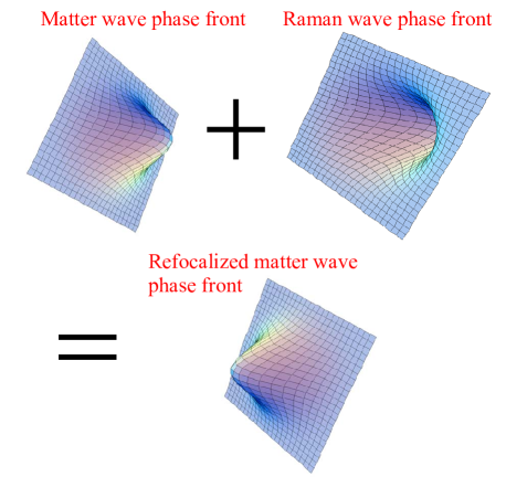
Figure 6: Interaction between a spherical matter wave and a laser. The laser spherical wave-front refocuses the matter wave.

Following up this intuitive picture, we propose an alternative matter-wave focusing scheme, fully original to our knowledge, based on the matter-wave interaction with electromagnetic fields of spherical wave-front. To show that the focusing is effective, we compute the transition amplitude of a matter wave interacting with Gaussian Raman waves to first order in the electromagnetic field. A similar computation has been previously performed by Bordé in the context of atomic beamsplitters Bordé (2004).

Let us consider for the “mirror pulse” two counterpropagating matched Gaussian beams:

$$E_{1}(x,y,z,t)=\frac{1}{2}U_{0}^{+}(\mathbf{r}-\mathbf{r_{w}})e^{ik_{0}(z-z_{w})}E(t)e^{i\omega_{1}t+i\varphi_{1}}+c.c$$

$$E_{2}(x,y,z,t)=\frac{1}{2}U_{0}^{-}(\mathbf{r}-\mathbf{r_{w}})e^{-ik_{0}(z-z_{w})}E(t)e^{i\omega_{2}t+i\varphi_{2}}+c.c$$

$$\mbox{with}\quad U_{0}^{\pm}(\mathbf{r})=\frac{1}{1\mp 2iz/b}\exp[-\frac{1}{1\mp 2iz/b}\frac{x^{2}+y^{2}}{w_{0}^{2}}]$$

where $k_{0}=(k_{2}-k_{1})/2$. The detuning $\omega_{2}-\omega_{1}$ is adjusted so that the relevant Raman process be the absorption of a photon from mode $E_{2}$ followed by the emission of a photon into mode $E_{1}$. We have used the confocal parameter of the light beam $b=k_{0}w_{0}^{2}$ as well as the complex Lorentzian function $L^{+}$ Bordé et al. (1976):

$$L^{+}(z)=\frac{1}{1-2iz/(k_{0}w_{0}^{2})}=\frac{1}{\sqrt{1+\frac{z^{2}}{4b^{2}}}}\exp[i\arctan\left(\frac{z}{2b}\right)]$$ (36)

The term $\arctan\left(\frac{z}{2b}\right)$ is known as the Gouy phase. The matching of the two laser beams is reflected in the relation between their transverse structures $U^{-}(\mathbf{r})=U^{+*}(\mathbf{r})$: at each point their curvature is identical. The Raman diffusion associated with these fields yields an effective interaction Hamiltonian whose matrix elements is:

$$V_{ba}(\mathbf{r},t)=-\hbar\Omega U_{0}^{+}(\mathbf{r}-\mathbf{r_{w}})U_{0}^{-*}(\mathbf{r}-\mathbf{r_{w}})e^{i2k_{0}(z-z_{w})}F(t)$$ (37)

$$\times e^{-i(\omega_{21}+r(t-t_{r}))t+i\varphi_{0}}+c.c.$$

The term $r(t-t_{r})$ accounts for the frequency ramp starting at time $t_{r}$, $\omega_{21}=\omega_{2}-\omega_{1}$ is the Raman detuning and $F(t)=|E(t)|^{2}$ the time envelope of the pulse. The computation of the transition amplitude is somewhat involved and deferred to Appendix D. We obtain:

$$b^{(1)}(\mathbf{r},t)=i\Omega\sqrt{2\pi}e^{i2k_{0}[z-z_{C0}(t)-2\hbar k_{0}(t-t_{0})/m]}e^{i\varphi^{\prime}_{0}}$$

$$\times L^{+}(z-z_{C0}(t))U_{0}^{+2}\left(\mathbf{r}-\mathbf{r_{C0}}(t)-\frac{2\hbar\mathbf{k_{0}}}{m}(t-t_{0})\right)$$

$$\times\langle b,\mathbf{r}|U_{0}(t,t_{0})\int\frac{d^{3}\mathbf{p}}{(2\pi\hbar)^{3/2}}\left[\tilde{F}(\omega_{B}(p_{z},\mathbf{k_{0}}))\langle a,\mathbf{p}|\Psi(t_{0})\rangle\right]|b,\mathbf{p}\rangle$$

$U_{0}(t,t_{0})$ is the evolution operator in the gravitational field, $\mathbf{r}_{C0}(t)=\mathbf{r_{w}}+\frac{\mathbf{p_{0}}}{m}(t-t_{0})+\frac{1}{2}\mathbf{g}(t-t_{0})^{2}$ and $\omega_{B}(p_{z},\mathbf{k_{0}})$ a frequency which reflects the Bragg resonance condition:

$$\omega_{B}(p_{z},\mathbf{k_{0}})=-[\omega_{ba}+\frac{\mathbf{k}\cdot\mathbf{p}}{m}+\frac{\hbar\mathbf{k}^{2}}{2m}-\omega_{21}+\mathbf{k}\cdot\mathbf{g}\>(t_{r}-t_{0})]$$ (39)

$U_{0}^{+2}(\mathbf{r})$ corresponds to a Gaussian mode of confocal parameter $b=k_{0}w_{0}^{2}$ and waist $w_{0}/\sqrt{2}$. The first-order term (D) is the leading contribution to the outgoing excited matter wave. The filtering of the pulse acts as expected through the Fourier envelope $\tilde{F}\left(\omega_{B}(p_{z},\mathbf{k_{0}})\right)$, significant only for a small velocity class which can be tuned by the starting time $t_{r}$ of the velocity ramp. The operator $U_{0}(t,t_{0})$ reflects the propagation in the gravitational field. The factor $L^{+}(z-z_{C}(t))$ barely affects the longitudinal shape of the atomic wave, without contributing to the average vertical momentum. As discussed in Section I, the cavity lifetime of the atomic sample does not depend on its longitudinal profile. Therefore we do not need to worry about this factor.

What matters is the transverse structure of this outgoing wave, which corresponds to a focusing matter wave. As suggested in Figure 6, the curvature of the Gaussian Raman wave has been transmitted from the laser wave to the atomic wave through the term $U_{0}^{+2}[\mathbf{r}-\mathbf{r_{C0}}(t)-\frac{2\hbar\mathbf{k_{0}}}{m}(t-t_{0})]$. This term induces a quadratic dependence of the phase on spatial coordinates:

$$U_{0}^{+2}(\mathbf{r})=\exp[-\frac{2k_{0}^{2}w_{0}^{2}+i4k_{0}z}{k_{0}^{2}w_{0}^{4}+4z^{2}}(x^{2}+y^{2})]$$ (40)

Following the approach of the precedent paragraph, and the relation (34), this can be interpreted as a thin lens effect. To express the corresponding focal, we introduce the vector $\tilde{\mathbf{r}}(t)=\mathbf{r}-\mathbf{r_{C0}}(t)-\frac{2\hbar\mathbf{k_{0}}}{m}(t-t_{0})$. For an atomic wave centered around $z=z_{a}$ at the time $t$, the interaction with the light field plays the role of a thin lens of focal $f(z_{a},z_{w},t)$ to first order in the electromagnetic field:

$$f(z_{a},z_{w},t)=\frac{m}{\hbar}\frac{k_{0}^{2}w_{0}^{4}+4\tilde{z}(t)^{2}}{8k_{0}\tilde{z}(t)}$$ (41)

where the parameter $\tilde{z}(t)$ is:

$$\tilde{z}(t)=z_{a}-\left(\frac{p_{0z}+2\hbar k_{0}}{m}(t-t_{0})-\frac{1}{2}g(t-t_{0})^{2}\right)-z_{w}$$ (42)

This focal can thus be controlled by the relative position of the laser waist and atomic wave-packet center. This first-order computation shows how the laser beam curvature is transferred to the matter beam wave-front and suggests that it is possible to focus matter waves through Raman pulses with a spherical wave-front in a controllable manner.

III.3 Transverse stability of the cavity

The main threat to the cavity stability is indeed the interatomic interactions which will push away the atoms of the sample from the central axis of the cavity. It is indeed possible to approximate these interactions with an effective lens. A detailed ABCD matrix analysis of interaction effects is given in ImpensABCDinteractions . Here we just consider that interactions induce an effective quadratic potential represented by the diagonal matrix $\gamma_{i}$.

In the precedent paragraphs, the focusing obtained is only effective for the transverse directions. This is sufficient, since the longitudinal spread of the atomic sample does not drive it out of the laser beams. The transverse stability of the cavity is entirely reflected in the temporal evolution of the Gaussian parameters $X(t),Y(t)$. The final parameters are related to the initial parameters by the ABCD matrix:

$$\left(\begin{array}[]{cc}\cosh[\sqrt{\gamma_{i}}T]-\frac{P_{\bot}}{f}\sqrt{\gamma_{i}}\sinh[\sqrt{\gamma_{i}}T]&{\gamma_{i}}^{-1/2}\sinh[\sqrt{\gamma_{i}}T]\\ \sqrt{\gamma_{i}}\sinh[\sqrt{\gamma_{i}}T]-\frac{P_{\bot}}{f}\cosh[\sqrt{\gamma_{i}}T]&\cosh[\sqrt{\gamma_{i}}T]\\ \end{array}\right)$$ (43)

As in ImpensABCDinteractions , one can use this input-output relation to model the stability of the matter-wave cavity. For the diluted matter waves involved in this system, a slight curvature in the mirror is sufficient to stabilize transversally the atomic beam.

IV Conclusion

We would like to point out the physical insight provided by the picture of a cavity in momentum space. Such a cavity is only possible in atom optics since photons, whose velocity is fixed to $c$, cannot be accelerated. In our system, the corresponding momentum wave-packet oscillates between two well-defined values (Fig. 2), with a resonance observed for the adequate time-spacing of the mirrors. We can push further the analogy with an optical cavity. The force $mg$ is the speed of the field in the momentum space. $4\hbar k$ is the momentum analog for the cavity length. The cycle period $T_{0}$ of the wave propagating in momentum space is orders of magnitude longer than the usual cycle time of a pulse in an optical cavity.

Let us look again at the resonance condition (1) with this picture in mind. This relation corresponds in momentum space to:

$$T=L/c$$ (44)

with the replacements $mg\rightarrow c$ (propagation velocity in momentum space) and $4\hbar k\rightarrow L$ (distance in momentum space). The usual resonance condition for an optical cavity yields:

$$T=nL/2c\quad n\in N$$ (45)

The difference can be explained by the fact that, unlike in an optical cavity where the light goes back and forth between the mirrors, the “way back” in momentum space from $-2\hbar k$ to $2\hbar k$ has to be provided by the light pulse. This explains why the factor $2$ is absent in the denominator of (44). The integer $n$ is absent in the resonance condition (44) because we considered only two-photon Raman pulses for the optical mirrors. Indeed, for each period $T_{n}=nT_{0}$, the cavity becomes resonant with mirror pulses based on $n$-photons processes. In order to levitate, the atomic sample needs to receive from the light pulse an adequate momentum transfer of $4n\hbar\mathbf{k}$. This momentum fixes the number of photons exchanged for each possible resonant period $T_{n}$.

In the proposed gravimeter, the momentum cavity is loaded with short single atomic pulses well-localized in momentum space, since the instantaneous velocity distribution is sharply peaked at any time. This is the analog of a femtosecond pulse propagating in an optical cavity. It would be interesting, however, to load the cavity with a continuous flow of free falling atoms coming from a continuous atom laser. At a fixed momentum, the contributions from different times would sum-up and interfere, exactly like in a Perot-Fabry interferometer. This system would then constitute to our knowledge the first example of a momentum space cavity continuously loaded with a matter-wave beam.

We have studied the levitation of an atomic sample by periodic double Raman pulses. In our system, the matter wave is trapped in an immaterial cavity of periodic optical mirrors. For the adequate time interspace between two pulses, the atomic sample is stabilized and levitate for a long time. Thanks to the sensitivity of the stabilization to this period, one obtains an accurate determination of the gravitational acceleration.

In our approach, the system could be loaded with any atomic sample describable by a macroscopic wave function. It is indeed not necessary to impose an initial small velocity dispersion, since the first mirror pulse will serve as a filter for a narrow velocity-class, while the next pulses will serve as a probe. Many aspects developed in this paper are still valid for a thermal cloud. Nonetheless, Bose Einstein condensates are ideally suited for this trap since matter-wave focusing is more efficient with a single mode coherent source. In this paper we have considered only $\pi$-pulses for the atom-light interactions. In fact, one could consider other schemes, for example one could split each $\pi$-pulse in two copropagating $\pi/2$-pulses separated by a dark space resulting in a sequence of Ramsey-Bordé interferometers MultiArches . Since the sensitivity to gravitation is proportional to the area covered in space-time by the interferometer, the optimal situation is obtained when the copropagating $\pi/2$-pulses are separated by $T_{0}/2$. An experimental realization of this proposal is planned with the support of the Institut Francilien de Recherche en Atomes Froids(IFRAF).

V Acknowledgements

We are very grateful to A. Landragin for valuable discussions and suggestions. This work is supported by CNRS, CNES, DGA, and ANR.

Appendix A Computation of the gravimeter sensitivity

After $n$ nearly-resonant cycles, the fraction of the cloud preserved becomes:

$$R(T)=R(p_{1})...R(p_{n})\quad\mbox{with}\quad R(p)=\frac{\sin^{4}\left(\frac{\pi}{2}\sqrt{1+y(p)^{2}}\right)}{(1+y(p)^{2})^{2}}$$ (46)

with expression (7) for the momenta:

$$p_{n}=-mgT/2+(n-1)\times mg(T_{0}-T)$$ (47)

At resonance $T=T_{0}$, one would have $p_{1}=..=p_{n}=-2\hbar k$ and $y(p_{1})=..=y(p_{n})=0$. For a big number of cycles $n$, in the vicinity of the resonance $T\simeq T_{0}$ one still has $y(p_{1}),...,y(p_{n})\ll 1$. The expression for the reflection coefficients simplifies to:

$$R(p_{i})=\frac{1}{(1+y^{2}(p_{i}))^{2}}+O(y^{4}(p_{i}))=1-2y^{2}(p_{i})+O(y^{4}(p_{i}))$$ (48)

The fraction of atoms kept in the cloud can then be expressed as:

$$\log\frac{1}{R(T)}=-\sum_{i=1}^{n}\log\left(R(p_{i})\right)\simeq\sum_{i=1}^{n}\log\left(1+2y^{2}(p_{i})\right)$$

We insert expression (7) for the momentum in (4) to derive an expression for the off-Braggness parameter:

$$y(p_{i})\simeq\frac{g(T-T_{0})k}{\Omega_{0}}\times i$$ (50)

The reflection coefficient becomes:

$$\log\frac{1}{R(T)}\simeq\sum_{i=1}^{n}\log\left(1+2i^{2}\frac{g^{2}(T-T_{0})^{2}k^{2}}{\Omega_{0}^{2}}\right)$$ (51)

This sum may be approximated by an integral because $i\gg 1$:

$$\log\frac{1}{R(T)}\simeq\int_{1}^{n}dx\log\left(1+2x^{2}\frac{g^{2}(T-T_{0})^{2}k^{2}}{\Omega_{0}^{2}}\right)$$ (52)

This integral can be performed analytically:

$$\int dx\log(1+ax^{2})=-2x+2\frac{\arctan(\sqrt{a}x)}{\sqrt{a}}+x\log(1+ax^{2})$$ (53)

We set $a=2g^{2}(T-T_{0})^{2}k^{2}/\Omega_{0}^{2}$, which verifies $\sqrt{a}n\simeq y(p_{n})\ll 1$. We can then use expression $(\ref{eq:integral})$ in $(\ref{eq:logR3})$ and Taylor expand the right hand side:

$$\log\frac{1}{R(T)}\simeq-2n+2[n-\frac{1}{3}an^{3}]+n\>an^{2}=\frac{1}{3}an^{3}$$ (54)

We have omitted the small term coming from the lower bound of the integral. We finally obtain:

$$\log\frac{1}{R(T)}=\frac{2g^{2}k^{2}(T-T_{0})^{2}n^{3}}{3\Omega_{0}^{2}}$$ (55)

Let the condensate perform $n$ bounces for a range of values of $T$ close to the expected value $T_{0}$, and detect the number of atoms in the cloud afterwards. If a relative variation $\epsilon$ can be tracked experimentally, we can bound the period $T_{0}$ between $T_{1}$ and $T_{2}$ such that $R(T_{1})=R(T_{2})=1-\epsilon$. According to our previous computation:

$$|T_{2}-T_{0}|\simeq|T_{1}-T_{0}|\simeq\sqrt{\frac{3\log(1/1-\epsilon)}{2}}\frac{\Omega_{0}}{gk}\frac{1}{n^{3/2}}$$ (56)

We infer the gravitational acceleration from the period $T_{0}$ thanks to relation (1), so that their relative errors are related by:

$$|\frac{\Delta g}{g}|\leq|\frac{\Delta T}{T}|+|\frac{\Delta v_{r}}{v_{r}}|$$ (57)

with the recoil velocity $v_{r}=\hbar k/m$. This gives the following upper bound for the relative error on the gravitational acceleration $g$:

$$\frac{|\Delta{g}|}{g}\leq\sqrt{\frac{3}{8}}\frac{1}{\hbar k^{2}}\left(\frac{\Omega_{0}\sqrt{-\log(1-\epsilon)}}{n^{3/2}}\right)+|\frac{\Delta v_{r}}{v_{r}}|$$ (58)

Appendix B Thomas-Fermi expansion

The evolution of a condensate initially in the strong coupling regime yields Castin and Dum (1996):

$$U_{TFE}(t,t_{0})|\Phi(t_{0})\rangle=|\Phi(t)\rangle$$ (59)

with:

$$\Phi(\mathbf{r},t)=\frac{e^{-i\beta(t)}e^{im\sum_{j}r_{j}^{2}\dot{\lambda}_{j}(t)/2\hbar\lambda_{j}(t)}}{\sqrt{\lambda_{1}(t)\lambda_{2}(t)\lambda_{3}(t)}}\tilde{\Phi}(\mathbf{r}/\lambda_{j}(t),t_{0})$$

$$\mbox{and}\>\tilde{\Phi}(\mathbf{r},t_{0})\simeq\left(\frac{\mu}{N_{0}g}\right)^{1/2}\left(1-\omega_{\bot}^{2}\frac{(x^{2}+y^{2})}{R^{2}}-\omega_{z}^{2}\frac{z^{2}}{Z^{2}}\right)^{1/2}$$

For a cigar-shaped condensate, the frequency ratio $\epsilon=\frac{\omega_{z}}{\omega_{\bot}}$ is small and we may keep track of the radial expansion only:

$$\lambda_{z}(t)=1\qquad\lambda_{\bot}(t)=\sqrt{1+\omega_{\bot}^{2}t^{2}}$$ (60)

$$\beta(t)=\frac{\mu}{\hbar\omega_{\bot}}\arctan\left(1+\omega_{\bot}^{2}t^{2}\right)$$ (61)

Appendix C Propagation of a wave function: the method of the generating function

Let us assume that we know the solution of a linear PDE for a family of initial conditions indexed by $\overrightarrow{\alpha}$:

$$\partial_{t}f(\mathbf{r},t,\overrightarrow{\alpha})=\L(f)(\mathbf{r},t,\overrightarrow{\alpha})$$

$$f(\mathbf{r},0,\overrightarrow{\alpha})=\frac{1}{\sqrt{\mbox{det}(X_{0})}}\exp[\frac{im}{2\hbar}(\mathbf{r}-\mathbf{r_{0}})Y_{0}X_{0}^{-1}(\mathbf{r}-\mathbf{r_{0}})$$

$$+\frac{i}{\hbar}(\mathbf{r}-\mathbf{r_{0}})\cdot(\mathbf{p_{0}}-2\hbar\tilde{X_{0}^{-1}}\overrightarrow{\alpha})+\frac{1}{2}\overrightarrow{\alpha}X_{0}^{-1}X_{0}^{*}\overrightarrow{\alpha}]=\Psi_{\overrightarrow{\alpha}}(\mathbf{r})$$

where $\L$ is a linear differential operator in the first two variables of the function $f$. Hermite modes can be defined through an analytic expansion of the exponential $\Psi_{\overrightarrow{\alpha}}(\mathbf{r})$:

$$\exp[\mathbf{r}M_{1}\mathbf{r}+\mathbf{r}M_{2}\overrightarrow{\alpha}+\overrightarrow{\alpha}M_{3}\overrightarrow{\alpha}]$$

$$=e^{\mathbf{r}M_{1}\mathbf{r}}\sum_{l,m,n}i^{l+m+n}\alpha_{1}^{l}\alpha_{2}^{m}\alpha_{3}^{n}H_{lmn}(\tilde{M_{2}}\mathbf{r},-\frac{1}{2}M_{3})$$

From the linearity of $\L$, the propagation of an Hermite-Gauss mode $H_{lmn}$, i.e. the solution at future times of the partial differential equation with initial condition:

$$\partial_{t}g_{lmn}(\mathbf{r},t)=\L(g_{lmn})(\mathbf{r},t)$$

$$g_{lmn}(\mathbf{r},0)=H_{lmn}(\mathbf{r})$$ (64)

can be inferred from the coefficient of $\alpha_{1}^{l}\alpha_{2}^{m}\alpha_{3}^{n}$ in the $\overrightarrow{\alpha}$ expansion of $f(\mathbf{r},t,\overrightarrow{\alpha})$, after a change of variables in the argument of the Hermite polynomial. The propagation of any arbitrary wave function $\Psi(\mathbf{r},t)$ then follows by linearity from the computation of the initial projection on the Hermite-Gauss basis:

$$\Psi(\mathbf{r},t)=\sum_{l,m,n}c_{lmn}\>g_{lmn}(\mathbf{r},t)$$

$$\mbox{with}\quad c_{lmn}=\int d^{3}\mathbf{r}H_{lmn}^{*}(\mathbf{r})\Psi(\mathbf{r},0)$$ (65)

Appendix D Computation of the first-order transition amplitude with spherical waves

The state vector evolves under the Hamiltonian $H=H_{0}+H_{E}+V$, where $H_{0}$ accounts for the internal atomic degrees of freedom, $H_{E}=p^{2}/2m+mgz$ for the external particle motion and $V$ for the light-field. In this appendix we compute the transition amplitude to first order in $V$. To perform this computation, we consider the state vector $|\tilde{\Psi}(t)\rangle$ in the interaction picture:

$$|\Psi(t)\rangle=U_{0}(t,t_{1})|\tilde{\Psi}(t)\rangle$$ (66)

$U_{0}(t,t_{1})$ is the free evolution operator in the absence of light field between times $t_{1}$ and $t$:

$$U_{0}(t,t_{1})=\exp\left(-iH_{E}(t-t_{1})/\hbar\right)\exp(-iH_{0}(t-t_{1})/\hbar)$$ (67)

The light field is turned on at time $t_{0}$. The first-order term of the Dyson series associated with the potential $V$ is:

$$|\tilde{\Psi}^{(1)}(t)\rangle=\frac{1}{i\hbar}\int_{t_{0}}^{t}dt^{\prime}\tilde{V}(t^{\prime})|\tilde{\Psi}^{(0)}(t_{0})\rangle$$ (68)

where $\tilde{V}(t^{\prime})$ is the potential in the interaction picture:

$$\tilde{V}(t)=U_{0}^{-1}(t,t_{1})\left(V_{ba}(\mathbf{r_{op}},t)\otimes|b\rangle\langle a|\right)U_{0}(t,t_{1})\>+\>h.c.$$

$$=V_{ba}\left(\mathbf{R_{op}}(t,t_{1}),t\right)\otimes|b\rangle\langle a|e^{i\omega_{ba}(t-t_{1})}\>+\>h.c.$$

$\mathbf{R_{op}}(t,t_{1})$ is the position operator in the interaction picture, given by integration of the Heisenberg equation of motion Bordé (2001b):

$$\mathbf{R_{op}}(t,t_{1})=U_{0}^{-1}(t,t_{1})\mathbf{r_{op}}U_{0}(t,t_{1})$$

$$=A(t,t_{1})\mathbf{r_{op}}+B(t,t_{1})\mathbf{p_{op}}+\mathbf{\xi}(t,t_{1})$$ (70)

The parameter $t_{1}$, associated with a choice of representation for the interaction picture, can be chosen as $t_{1}=t_{0}$. We need only consider the term $V_{ba}$ of the interaction potential, for which we adopt the usual rotating wave approximation. The first-order transition amplitude $b^{(1)}(\mathbf{r},t)$ is given by the relation:

$$b^{(1)}(\mathbf{r},t)=\frac{1}{i\hbar} \langle b,\mathbf{r}|U_{0}(t,t_{0})\int_{t_{0}}^{t}dt^{\prime}V_{ba}\left(\mathbf{R_{op}}(t^{\prime},t_{0}),t^{\prime}\right)\otimes|b\rangle\langle a|$$ (71)

$$\times e^{i\omega_{ba}(t-t_{0})}U^{-1}_{0}(t_{0},t_{0})|\Psi(t_{0})\rangle$$

In order to understand how the light wave structures the atomic wave-packet, we introduce the matrix elements of $V$ between plane atomic waves:

$$b(\mathbf{r},t)=\frac{1}{i\hbar}\langle b,\mathbf{r}|U_{0}(t,t_{0})\int_{t_{0}}^{t}dt^{\prime}\frac{d\mathbf{p}d\mathbf{p^{\prime}}}{(2\pi\hbar)^{3}}|b,\mathbf{p^{\prime}}\rangle e^{i\omega_{ba}(t^{\prime}-t_{0})}$$

$$\times\langle\mathbf{p^{\prime}}|V_{ba}\left(\mathbf{R_{op}}(t^{\prime},t_{0}),t^{\prime}\right)|\mathbf{p}\rangle e^{i\omega_{ba}(t^{\prime}-t_{0})}\langle a,\mathbf{p}|\Psi(t_{0})\rangle$$

We introduce the Fourier transform of the interaction potential:

$$V_{ba}(\mathbf{r},t)=-\hbar\Omega F(t)e^{-i\frac{r}{2}(t-t_{r})^{2}-i\omega_{21}(t-t_{0})+i\varphi_{0}}$$

$$\times\int\frac{d^{3}\mathbf{k}}{(2\pi)^{3/2}}W(\mathbf{k})e^{i\mathbf{k}\cdot(\mathbf{r}-\mathbf{r_{w}})}$$

To compute the Fourier components of $V$, we first use the BCH relation:

$$e^{i\mathbf{k}\cdot(A(t^{\prime},t_{0})\mathbf{r_{op}}+B(t^{\prime},t_{0})\mathbf{p_{op}}+\xi(t^{\prime},t_{0}))}=e^{i\mathbf{k}\cdot A(t^{\prime},t_{0})\mathbf{r_{op}}}e^{i\mathbf{k}\cdot B(t^{\prime},t_{0})\mathbf{p_{op}}}$$

$$\times e^{\frac{1}{2}[\tilde{A}(t^{\prime},t_{0})\mathbf{k}\cdot\mathbf{r_{op}},\tilde{B}(t^{\prime},t_{0})\mathbf{k}\cdot\mathbf{p_{op}}]+i\xi(t^{\prime},t_{0}))}$$

The last commutator is responsible for the recoil term, and can be written:

$$\frac{1}{2}[\tilde{A}(t^{\prime},t_{0})\mathbf{k}\cdot\mathbf{r_{op}},\tilde{B}(t^{\prime},t_{0})\mathbf{k}\cdot\mathbf{p_{op}}]=\frac{i\hbar}{2}\tilde{\mathbf{k}}A(t^{\prime},t_{0})\tilde{B}(t^{\prime},t_{0})\mathbf{k}$$ (75)

The matrix element of the interaction potential contains the following term:

$$\langle\mathbf{p^{\prime}}|W(\mathbf{k})e^{i\mathbf{k}\cdot(A(t^{\prime},t_{0})\mathbf{r_{op}}+B(t^{\prime},t_{0})\mathbf{p_{op}}+\xi(t^{\prime},t_{0}))}|\mathbf{p}\rangle$$

$$=W(\mathbf{k})e^{i\mathbf{k}\cdot B\mathbf{p}-i\frac{\hbar}{2m}\tilde{\mathbf{k}}A\tilde{B}\mathbf{k}+i\xi}\langle\mathbf{p^{\prime}}|e^{i\tilde{A}\mathbf{k}\cdot\mathbf{r_{op}}}|\mathbf{p}\rangle$$

$$=W(\mathbf{k})e^{i\mathbf{k}\cdot B\mathbf{p}+i\frac{\hbar}{2m}\tilde{\mathbf{k}}A\tilde{B}\mathbf{k}+i\xi}\delta(\mathbf{p^{\prime}}-\mathbf{p}-\hbar\tilde{A}\mathbf{k})$$ (76)

we omitted the $(t^{\prime},t_{0})$ to alleviate the notations. The transition amplitude (D) becomes:

$$b^{(1)}(\mathbf{r},t)=i\Omega\int\frac{d^{3}\mathbf{p}d^{3}\mathbf{k}}{(2\pi\hbar)^{3/2}(2\pi)^{3/2}}\int_{t_{0}}^{t}dt^{\prime}\langle b,\mathbf{r}|U_{0}(t,t_{0})|b,\mathbf{p}+\hbar\tilde{A}(t^{\prime},t_{0})\mathbf{k}\rangle W(\mathbf{k})e^{i\mathbf{k}\cdot(B(t^{\prime},t_{0})\mathbf{p}+i\xi(t^{\prime},t_{0})-\mathbf{r_{w}})}$$

$$\times e^{i\frac{\hbar}{2m}\tilde{\mathbf{k}}A(t^{\prime},t_{0})\tilde{B}(t^{\prime},t_{0})\mathbf{k}}e^{i\omega_{ba}(t^{\prime}-t_{0})}F(t^{\prime})e^{-i\frac{r}{2}(t^{\prime}-t_{r})^{2}-i\omega_{21}(t^{\prime}-t_{0})+i\varphi_{0}}\langle a,\mathbf{p}|\Psi(t_{0})\rangle$$ (77)

The evolution of the $ABCD\xi$ parameters in a constant gravitational field is simple:

$$A(t^{\prime},t_{0})=1\quad B(t^{\prime},t_{0})=\frac{t^{\prime}-t_{0}}{m}\quad\xi(t^{\prime},t_{0})=\frac{1}{2}\mathbf{g}(t^{\prime}-t_{0})^{2}$$ (78)

One can extend the computation to include the effect of interactions by taking into account an effective lensing effect in the $ABCD$ matrices. This approach will be developed elsewhere. We introduce the Fourier transform $\tilde{F}(\omega)=\int\frac{dt}{\sqrt{2\pi}}F(t)e^{-i\omega t}$ of the slowly varying envelope $F(t^{\prime})$. The phase in the integral (D) is a second-order polynomial in $t^{\prime}$:

$$\varphi(t^{\prime})=\frac{1}{2}(\mathbf{k}\cdot\mathbf{g}-r){t^{\prime}}^{2}+[\omega_{ba}+\frac{\mathbf{k}\cdot\mathbf{p}}{m}+\frac{\hbar\mathbf{k}^{2}}{2m}-\omega_{21}+r\>t_{r}-\mathbf{k}\cdot\mathbf{g}\>t_{0}+\omega]t^{\prime}+\varphi^{\prime}_{0}$$ (79)

where $\varphi^{\prime}_{0}$ is a constant phase term. In order to maximize the transition amplitude, the chirp rate $r$ should be adjusted to cancel the quadratic variation of the phase, which yields as anticipated in Section I:

$$r=\mathbf{k}\cdot\mathbf{g}$$ (80)

The time $t_{r}$, at which the frequency ramp begins, selects the velocity class of the atoms which undergo the transition. Indeed, the momentum $p$ of these atoms satisfies:

$$|\omega_{ba}+\frac{\mathbf{k}\cdot\mathbf{p}}{m}+\frac{\hbar\mathbf{k}^{2}}{2m}-\omega_{21}+\mathbf{k}\cdot\mathbf{g}\>(t_{r}-t_{0})|\leq\Delta\omega$$ (81)

where $\Delta\omega$ is the spectral width of the time envelope $F(t^{\prime})$. As a consistency check, we see that this condition reproduces the resonance condition (I.3) for $t_{r}=t_{0}$. The next step in the computation of the amplitude (D) is to consider that the matter wave is out of the interaction zone at the initial and final times. This is legitimate, since we are in fact interested in computing a scattering amplitude. This simplification allows us to extend the bounds of the time integral to infinity, which yields a Dirac distribution:

$$b^{(1)}(\mathbf{r},t)=i\Omega\sqrt{2\pi}e^{i\varphi^{\prime}_{0}}\int\frac{d^{3}\mathbf{p}d^{3}\mathbf{k}}{(2\pi\hbar)^{3/2}(2\pi)^{3/2}}\langle b,\mathbf{r}|U_{0}(t,t_{0})|b,\mathbf{p}+\hbar\mathbf{k}\rangle$$

$$\times W(\mathbf{k})e^{-i\mathbf{k}\cdot\mathbf{r_{w}}}\langle a,\mathbf{p}|\Psi(t_{0})\rangle\int d\omega\tilde{F}(\omega)\delta\left(\omega+\omega_{ba}+\frac{\mathbf{k}\cdot\mathbf{p}}{m}+\frac{\hbar\mathbf{k}^{2}}{2m}-\omega_{21}+\mathbf{k}\cdot\mathbf{g}\>(t_{r}-t_{0})\right)$$ (82)

The Bragg resonance condition selects the Fourier component of adequate frequency in the temporal envelope. To alleviate the notations, we note $\omega_{B}(\mathbf{p},\mathbf{k})$ the frequency selected by the Bragg condition:

$$\omega_{B}(\mathbf{p},\mathbf{k})=\omega_{ba}+\frac{\mathbf{k}\cdot\mathbf{p}}{m}+\frac{\hbar\mathbf{k}^{2}}{2m}-\omega_{21}+\mathbf{k}\cdot\mathbf{g}\>(t_{r}-t_{0})$$ (83)

To simplify the computation, it is useful to assume that the spectrum $\tilde{F}(\omega)$ is broad enough to override dispersion effects of the laser wave. In other words:

$$\omega_{B}(\mathbf{p},\mathbf{k})\simeq\omega_{B}(p_{z},\mathbf{k_{0}})$$ (84)

This is legitimate if the spectral width $\Delta\omega$ of the pulse $F(t)$ verifies:

$$\Delta\omega\gg\Delta k_{z}\>\frac{p_{0}}{m},\Delta k_{\bot}\frac{\Delta{p_{\bot}}}{m}$$ (85)

Within these conditions, the Dirac integral leaves the amplitude:

$$b^{(1)}(\mathbf{r},t)=i\Omega\sqrt{2\pi}e^{i\varphi^{\prime}_{0}}\int\frac{d^{3}\mathbf{p}d^{3}\mathbf{k}}{(2\pi\hbar)^{3/2}(2\pi)^{3/2}}\langle b,\mathbf{r}|U_{0}(t,t_{0})|b,\mathbf{p}+\hbar\mathbf{k}\rangle W(\mathbf{k})e^{-i\mathbf{k}\cdot\mathbf{r_{w}}}\tilde{F}(\omega_{B}(p_{z},\mathbf{k_{0}}))\langle a,\mathbf{p}|\Psi(t_{0})\rangle$$ (86)

In order to see how the curvature of the light beam is imprinted onto the atomic beam, we need to perform the integration over $W(\mathbf{k})$. To compute this spatial Fourier transform, we go back to the expression of the potential (37):

$$V_{ba}(\mathbf{r},t)=-\hbar\Omega U_{0}^{+2}(\mathbf{r}-\mathbf{r_{w}})e^{i2k_{0}(z-z_{w})}F(t)e^{-i(\omega_{21}+r(t-t_{r}))t}+c.c.$$ (87)

where we have used the relation between the Gaussian modes $U^{+}(\mathbf{r})=U^{-*}(\mathbf{r})$. The spatial function inside the potential is defined by:

$$U_{0}^{+}(\mathbf{r})=\frac{1}{1-2iz/b}\exp\left[-\frac{1}{1-2iz/b}\frac{x^{2}+y^{2}}{w_{0}^{2}}\right]$$ (88)

with the confocal parameter $b=k_{0}w_{0}^{2}$. It will be useful to introduce its transverse Fourier transform:

$$U_{0}^{+}(\mathbf{r})=\frac{w_{0}^{2}}{4\pi}\int dk_{x}dk_{y}\exp\left[-\frac{(k_{x}^{2}+k_{y}^{2})w_{0}^{2}}{4}(1-2iz/b)\right]$$ (89)

It is convenient to introduce the Lorentzian function Bordé et al. (1976):

$$L^{+}(z)=\frac{1}{1-2iz/b}$$ (90)

The transverse Fourier transform of $W(\mathbf{r})$ can then be expressed as:

$$W(\mathbf{r})={L^{+}}^{2}(z)\exp\left[-2L^{+}(z)\frac{x^{2}+y^{2}}{w_{0}^{2}}\right]e^{i2k_{0}z}=\int\frac{d^{2}k_{\bot}}{(2\pi)}\left(\frac{w_{0}^{2}}{4}L^{+}(z)\exp\left[-\frac{(k_{x}^{2}+k_{y}^{2})}{4}\frac{w_{0}^{2}}{2}(1-2iz/b)\right]e^{i2k_{0}z}\right)e^{ik_{\bot}\cdot\mathbf{r_{\bot}}}$$

From this last expression we infer:

$$\int\frac{dk_{z}}{(2\pi)^{1/2}}W(\mathbf{k})e^{ikz}=L^{+}(z)\frac{w_{0}^{2}}{4}\exp\left[-\frac{(k_{x}^{2}+k_{y}^{2})}{4}\frac{w_{0}^{2}}{2}(1-2iz/b)\right]e^{+i2k_{0}z}$$ (92)

The propagation of a plane wave in a gravitational field yields:

$$\langle\mathbf{r}|U_{0}(t,t_{0})|\mathbf{p}\rangle=\frac{1}{\sqrt{2\pi\hbar}}e^{\frac{i}{\hbar}\mathbf{p}\cdot\mathbf{r}}e^{iS_{Cl}(t,t_{0})}$$ (93)

with $S_{Cl}(t,t_{0})$ classical action between a trajectory of initial momentum $\mathbf{p}$, final position $\mathbf{r}$ and duration $t-t_{0}$. The corresponding expression can be recast as:

$$\langle\mathbf{r}|U_{0}(t,t_{0})|\mathbf{p}\rangle=\frac{1}{\sqrt{2\pi\hbar}}e^{-img^{2}(t-t_{0})^{3}/6\hbar}e^{-\frac{i}{2\hbar}\mathbf{p}\cdot\mathbf{g}(t-t_{0})^{2}}e^{\frac{i}{\hbar}(\mathbf{p}-m\mathbf{g}(t-t_{0}))\cdot\mathbf{r}}e^{-i\mathbf{p}^{2}(t-t_{0})/2m}$$ (94)

This gives an expression for the matrix element:

$$\langle b,\mathbf{r}|U_{0}(t,t_{0})|b,\mathbf{p}+\hbar\mathbf{k}\rangle=\frac{1}{\sqrt{2\pi\hbar}}e^{-img^{2}(t-t_{0})^{3}/6\hbar}e^{-\frac{i}{2\hbar}\mathbf{p}\cdot\mathbf{g}(t-t_{0})^{2}}\cdot e^{\frac{i}{\hbar}(\mathbf{p}-m\mathbf{g}(t-t_{0}))\cdot\mathbf{r}}e^{i\mathbf{k}\cdot(\mathbf{r}-\frac{1}{2}\mathbf{g}(t-t_{0})^{2}-\frac{\mathbf{p}}{m}(t-t_{0})-\mathbf{r_{w}})}$$

$$\times e^{-i\omega_{b}(t-t_{0})}e^{-i\hbar\mathbf{k_{z}}^{2}/2m(t-t_{0})}e^{-i\mathbf{p}^{2}(t-t_{0})/2m}e^{-i\hbar\mathbf{k_{\bot}}^{2}(t-t_{0})/2m}$$ (95)

The momentum distribution $W(\mathbf{k})$ peaked around the value $\mathbf{k}=2k_{0}\mathbf{u_{z}}$ has a width $\Delta\mathbf{k}\ll k_{0}$, and one can verify on (D) that its longitudinal width $\Delta k_{z}$ is much narrower than the transverse ones $\Delta k_{x},\Delta k_{y}$. The correction to the longitudinal recoil $\hbar k_{z}^{2}/2m$ when $\mathbf{k}$ varies in the width of $W(\mathbf{k})$ is thus typically much smaller than the transverse recoil. The term $\hbar k_{z}^{2}/2m$ in equation (D) will therefore be approximated by $2\hbar k_{0}^{2}/m$. By summing up the Fourier modes, we will recover for the atomic wave the transverse Fourier profile of the Gaussian laser wave $(\ref{eq:W(r)Fouriertransform})$ up to a translation. We note $\mathbf{r_{c}}(t)=\mathbf{r_{w}}+\frac{\mathbf{p}}{m}(t-t_{0})+\frac{1}{2}\mathbf{g}(t-t_{0})^{2}$ the point associated with a classical motion in the gravity field from $\mathbf{r_{w}}$. The role played by the position associated with the classical movement and the action phase pre-factor are indeed a consequence of the $ABCD\xi$ theorem Bordé (2001a). Gathering all the terms of (86) dependent on the wave-vector $\mathbf{k}$, and using relation (92)we can perform the integration on the wavevector $\mathbf{k}$ along:

$$\int\frac{d^{2}\mathbf{k}_{\bot}}{(2\pi)}\left[\int\frac{dk_{z}}{(2\pi)^{1/2}}W(\mathbf{k})e^{ik_{z}(z-z_{C})}\right]e^{i\mathbf{k_{\bot}}\cdot(\mathbf{r_{\bot}}-\mathbf{r_{C\bot}})}e^{-i\frac{\hbar\mathbf{k_{\bot}}^{2}}{2m}(t-t_{0})}e^{-i\frac{2\hbar k_{0}^{2}}{m}(t-t_{0})}$$

$$= L^{+}(z-z_{C}(t))e^{i2k_{0}(z-z_{C})}e^{-i\frac{2\hbar k_{0}^{2}}{m}(t-t_{0})}\frac{w_{0}^{2}}{4}\int\frac{d^{2}\mathbf{k}_{\bot}}{(2\pi)}\exp\left[-\frac{\mathbf{k_{\bot}}^{2}}{4}\frac{w_{0}^{2}}{2}(1-2i(z-z_{C})/b)\right]e^{-i\frac{\hbar\mathbf{k_{\bot}}^{2}}{2m}(t-t_{0})}e^{i\mathbf{k_{\bot}}\cdot(\mathbf{r_{\bot}}-\mathbf{r_{C\bot}}(t))}$$

$$= L^{+}(z-z_{C}(t))e^{i2k_{0}[z-z_{C}-2\hbar k_{0}(t-t_{0})/m]}\frac{w_{0}^{2}}{4}\int\frac{d^{2}\mathbf{k}_{\bot}}{(2\pi)}\exp\left[-\frac{\mathbf{k}_{\bot}^{2}}{8}w_{0}^{2}\left(1-\frac{2i}{k_{0}w_{0}^{2}}(z-z_{C}(t)-\frac{2\hbar k_{0}(t-t_{0})}{m}\right)\right]e^{i\mathbf{k_{\bot}}\cdot(\mathbf{r_{\bot}}-\mathbf{r_{C\bot}}(t))}$$

$$= L^{+}(z-z_{C}(t))e^{i2k_{0}[z-z_{C}(t)-\frac{2\hbar k_{0}}{m}(t-t_{0})]}U_{0}^{+2}\left(\mathbf{r}-\mathbf{r_{C}}(t)-\frac{2\hbar\mathbf{k_{0}}}{m}(t-t_{0})\right)$$

The momentum acquired during the Raman process is reflected in the factor $e^{i2k_{0}[z-z_{C}(t)-\frac{2\hbar k_{0}}{m}(t-t_{0})]}$. The translation $\mathbf{r}-\mathbf{r_{C}}(t)-\frac{2\hbar\mathbf{k_{0}}}{m}(t-t_{0})$ accounts for the classical motion in the gravitational field and the momentum acquired during the Raman process. Inserting this result in the equation (86):

$$b^{(1)}(\mathbf{r},t) = i\Omega\sqrt{2\pi}e^{i2k_{0}[z-z_{C0}(t)-2\hbar k_{0}(t-t_{0})/m]}e^{i\varphi^{\prime}_{0}}$$

$$\times \int\frac{d^{3}\mathbf{p}}{(2\pi\hbar)^{3/2}}e^{-img^{2}(t-t_{0})^{3}/6\hbar}e^{-\frac{i}{2\hbar}\mathbf{p}\cdot\mathbf{g}(t-t_{0})^{2}}e^{-i\mathbf{p}^{2}(t-t_{0})/2m}e^{\frac{i}{\hbar}(\mathbf{p}-m\mathbf{g}(t-t_{0}))\cdot\mathbf{r}}e^{-i\omega_{b}t}$$

$$\times L^{+}(z-z_{C}(t))U_{0}^{+2}\left(\mathbf{r}-\mathbf{r_{C0}}(t)-\frac{2\hbar\mathbf{k_{0}}}{m}(t-t_{0})\right)\tilde{F}(\omega_{B}(p_{z},\mathbf{k_{0}}))\langle a,\mathbf{p}|\Psi(t_{0})\rangle$$

If the atomic wave-packet is sufficiently narrow, the Gaussian modes $L^{+}(z-z_{C}(t))U_{2}^{+}\left(\mathbf{r}-\mathbf{r_{C}}(t)-\frac{2\hbar\mathbf{k_{0}}}{m}(t-t_{0})\right)$, which depend on the momentum $\mathbf{p}$ through $r_{C}(t)$, are approximately constant on the width of the distribution $\tilde{F}(\omega_{B}(p_{z},\mathbf{k_{0}}))\langle a,\mathbf{p}|\Psi(t_{0})\rangle$ centered on $\mathbf{p_{0}}$. We can then pull those functions out of the momentum integral. The phase factor in the momentum integral correspond to the propagation of plane waves in a gravitational field. One can thus interpret the momentum integral as the propagation of the filtered wave-packet in the gravitational field:

$$b^{(1)}(\mathbf{r},t)=i\Omega\sqrt{2\pi}e^{i2k_{0}[z-z_{C0}(t)-2\hbar k_{0}(t-t_{0})/m]}e^{i\varphi^{\prime}_{0}}L^{+}(z-z_{C0}(t))U_{0}^{+2}\left(\mathbf{r}-\mathbf{r_{C0}}(t)-\frac{2\hbar\mathbf{k_{0}}}{m}(t-t_{0})\right)$$

$$\times\langle b,\mathbf{r}|U_{0}(t,t_{0})\int\frac{d^{3}\mathbf{p}}{(2\pi\hbar)^{3/2}}\left[\tilde{F}(\omega_{B}(p_{z},\mathbf{k_{0}}))\langle a,\mathbf{p}|\Psi(t_{0})\rangle\right]|b,\mathbf{p}\rangle$$

with $\mathbf{r}_{C0}(t)=\mathbf{r_{w}}+\frac{\mathbf{p_{0}}}{m}(t-t_{0})+\frac{1}{2}\mathbf{g}(t-t_{0})^{2}$. To first order in the field, the curvature of the Gaussian Raman wave is transferred in a controlled way to the atomic wave through the terms $L^{+}(z-z_{C0}(t))U_{0}^{+2}\left(\mathbf{r}-\mathbf{r_{C0}}(t)-\frac{2\hbar\mathbf{k_{0}}}{m}(t-t_{0})\right)$.

References

• Peters et al. (1999) A. Peters, K. Y. Chung, and S. Chu, Nature 400, 849 (1999).
• Peters et al. (2001) A. Peters, K. Y. Chung, and S. Chu, Metrologia 38, 25 (2001).
• Cladé et al. (2005) P. Cladé, S. Guellati-Khelifa, C. Schwob, F. Nez, L. Julien, and F. Biraben, Europhysics Letters 71, 730, arXive/0506225 (2005).
• Bordé et al. (1987) C. J. Bordé, C. Chardonnet, and D. Mayou, Laser Spectroscopy VIII, eds W. Persson and S. Svanberg, Springer Verlag pp. 381–385 (1987).
• Wallis et al. (1992) H. Wallis, J. Dalibard, and C. Cohen-Tannoudji, Appl. Phys. B 54, 407 (1992).
• Aminoff et al. (1993) C. G. Aminoff, A. M. Steane, P. Bouyer, P. Desbiolles, J. Dalibard, and C. Cohen-Tannoudji, Phys. Rev. Lett. 71, 3083 (1993).
• Landragin et al. (1996) A. Landragin, J.-Y. Courtois, G. Labeyrie, N. Vansteenkiste, C. I. Wesbrook, and A. Aspect, Phys. Rev. Lett. 77, 1464 1467 (1996).
• Impens et al. (2006) F. Impens, P. Bouyer, A. Landragin, and C. J. Bordé, to appear in Journal de Physique IV (2006).
• Weitz et al. (1994) M. Weitz, B. C. Young, and S. Chu, Phys. Rev. Lett. 73, 2563 (1994).
• Bordé (1997) C. J. Bordé, Matter wave interferometers: a synthetic approach in Atom Interferometry, edited by P. Berman, Academic Press pp. 257–292 (1997).
• Coq et al. (2001) Y. L. Coq, J. H. Thywissen, S. A. Rangwala, F. Gerbier, S. Richard, G. Delannoy, P. Bouyer, and A. Aspect, Phys. Rev. Lett. 87, 170403 (2001).
• Weiss et al. (1993) D. S. Weiss, B. C. Young, and S. Chu, Phys. Rev. Lett. 70, 2706 2709 (1993).
• Wicht et al. (2002) A. Wicht, J. Hensley, E. Sarajlic, and S. Chu, Physica Scripta 102, 82 (2002).
• Battesti et al. (2004) R. Battesti, P. Cladé, S. Guellati-Khelifa, C. Schwob, F. Nez, L. Julien, and F. Biraben, Phys. Rev. Lett. 92, 253001 (2004).
• Bordé (1992) C. J. Bordé, Les Houches, Session LIII 1990, Fundamental Systems in Quantum Optics (1992).
• Bordé (2001a) C. J. Bordé, C. R. Acad. Sci Paris Série IV pp. 509–530 (2001a).
• Bordé (2001b) C. J. Bordé, Metrologia 39, 435 (2001b).
• Castin and Dum (1996) Y. Castin and R. Dum, Phys. Rev. Lett. 77, 5315 5319 (1996).
• Bordé and Lämmerzahl (1995) C. J. Bordé and C. Lämmerzahl, Phys. Lett. A 203, 59 (1995).
• Bongs et al. (1999) K. Bongs, S. Burger, G. Birkl, K. Sengstock, W. Ertmer, K. Rz a zewski, A. Sanpera, and M. Lewenstein, Phys. Rev. Lett. 83, 3577 (1999).
• Arnold et al. (2002) A. S. Arnold, C. MacCormick, and M. G. Boshier, Phys. Rev. A 65, 031601 (2002).
• Saba et al. (1999) C. V. Saba, P. A. Barton, M. G. Boshier, I. G. Hughes, P. Rosenbusch, B. E. Sauer, and E. A. Hinds, Phys. Rev. Lett. 82, 468 (1999).
• Whyte et al. (2004) G. Whyte, P. Öhberg, and J. Courtial, Phys. Rev. A 69, 053610 (2004).
• Bordé (2004) C. J. Bordé, General Relativity and Gravitation 36, 475 (2004).
• Bordé et al. (1976) C. J. Bordé, J. L. Hall, C. V. Kunasz, and D. G. Hummer, Phys. Rev. A 14, 236 (1976).
• (26) F. Impens and Ch. J. Bordé, eprint arXiv:0709.3381.
• (27) F. Impens and Ch. J. Bordé, eprint arXiv:0808.3380; C. J. Bordé and F. Impens, in Abs. of ICOLS 2007 www.laserspectroscopy.org, (2007); F. Impens et. al. in Abs. of YAO 2007 (2007).