First nonlinear force-free field extrapolations of SOLIS/VSM data

Abstract

Aims. We study the coronal magnetic field structure inside active regions and its temporal evolution. We attempt to compare the magnetic configuration of an active region in a very quiet period with that for the same region during a flare.

Methods. Probably for the first time, we use vector magnetograph data from the Synoptic Optical Long-term Investigations of the Sun survey (SOLIS) to model the coronal magnetic field as a sequence of nonlinear force-free equilibria. We study the active region NOAA 10960 observed on 2007 June 7 with three snapshots taken during a small C1.0 flare of time cadence 10 minutes and six snapshots during a quiet period.

Results. The total magnetic energy in the active region was approximately $3\times 10^{25}$ J. Before the flare the free magnetic energy was about 5 % of the potential field energy. A part of this excess energy was released during the flare, producing almost a potential configuration at the beginning of the quiet period.

Conclusions. During the investigated period, the coronal magnetic energy was only a few percent higher than that of the potential field and consequently only a small C1.0 flare occurred. This was compared with an earlier investigated active region 10540, where the free magnetic energy was about 60 % higher than that of the potential field producing two M-class flares. However, the free magnetic energy accumulates before and is released during the flare which appears to be the case for both large and small flares.

1 Introduction

Methods have been developed to extrapolate the observed photospheric magnetic field vector into the corona. Using the fact that the magnetic field is dominant in solar active regions (ARs), we are able to neglect non-magnetic forces and to assume that the coronal magnetic field is force-free. Different instruments provide photospheric vector magnetograph data, which are used as input to the extrapolation methods. These data have, however had a rather low time cadence. Data of high time cadence are required to investigate in detail, for example the different evolutionary stages of solar flares. Suitable data include magnetic field observations of the Sun provided by the SOLIS Vector-SpectroMagnetograph. With a time cadence of $\approx$ 10 minutes, the instrument is designed to measure multiple area scans of ARs, which enables us for the first time to investigate the evolution of the coronal magnetic field energy with a high time cadence. Many existing studies deal with the extrapolation based on vector magnetograph data. For instance, Régnier & Priest (2007) dealt with the photospheric vector magnetic field provided by the Mees Solar Observatory Imaging Vector Magnetograph, Wiegelmann et al. (2005) used spectropolarimetric data recorded with the Tenerife Infrared Polarimeter of the German Vacuum Tower Telescope, and Thalmann & Wiegelmann (2008) performed extrapolations of Solar Flare Telescope Vector Magnetograph data. In all of these studies, only one snapshot was however used or, as in the last of the aforementioned studies, a sequence of vector magnetograms with a low time cadence of one magnetogram per day. Therefore, an improvement is achieved by applying our extrapolation technique to the high time cadence SOLIS/VSM data as described in the present study.

2 Method

2.1 Instrumentation: The SOLIS/VSM instrument

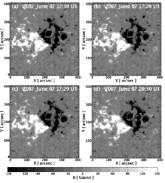
Figure 1: Longitudinal component of the SOLIS/VSM data during the C1.0 flare in panels (a) – (c) and after the flare in panel (d).

The Vector-SpectroMagnetograph (VSM; see Jones et al., 2002) on the Synoptic Optical Long-term Investigations of the Sun (SOLIS; see Keller et al., 2003) has provided magnetic field observations of the Sun almost continuously since August 2003. The instrument is designed to measure the magnetic field vector everywhere on the solar disk. Full disk vector observations are completed at least weekly. Multiple areas scans of ARs have also been available since November 2006. In addition, longitudinal magnetic field measurements in the photosphere (at the Fe i 630.15 nm and 630.25 nm spectral lines) and chromosphere (at the Ca ii 854.2 nm spectral line) are available on a daily basis. Quick-look data (JPEG images and FITS files) of the magnetic field vector in and around automatically selected ARs (Georgoulis et al., 2008) are available online to the community. The Quick-look data provides estimates of the magnetic field strength, inclination, and azimuth (Henney et al., 2006, and references therein), which should, because of the high field strength in ARs, be comparable to fully inverted data only differing by a few percent. The azimuth 180^∘-ambiguity is solved using the Nonpotential Magnetic Field Calculation method (NPFC; see Georgoulis, 2005), which does not introduce any error in the azimuth or any other quantities. Tools for full Milne-Eddington inversion are being developed to provide more accurate magnetic data especially in weak field regions.
In the time period around an C1.0 flare on 2007 June 7, three SOLIS/VSM vector magnetograms were available to use. One in the rising phase of the emission, one at the time when the flare peaked, and one in its decaying phase (at 17:10 UT, 17:20 UT, and 17:29 UT as shown in panel (a), (b), and (c) in Fig. 1, respectively). All the other magnetic field measurements on 2007 June 7 (between 20:30 UT and 21:42 UT) allow us to investigate the magnetic field structure in a period of low solar activity.

2.2 Numerics: Nonlinear force-free extrapolation

The basic equations for the computation of the nonlinear force-free magnetic field vector $\mathbf{B}$ are

$$(\nabla\times\mathbf{B})\times\mathbf{B}=0,$$ (1)

$$\nabla\cdot\mathbf{B}=0,$$ (2)

where Eq. (1) expresses that the Lorentz force is forced to vanish (as a consequence of j $\parallel$ B, where j is the electric current density) and Eq. (2) describes the absence of magnetic monopoles. For reviews on how to solve these equations, we refer the reader for example to Sakurai (1989), Amari et al. (1997), and Wiegelmann (2008).
A special form of the force-free fields are potential magnetic fields which can be computed from the longitudinal photospheric magnetic field alone and correspond to the minimum energy state for given boundary conditions. We calculate the potential field with the help of a Fast-Fourier method (Alissandrakis, 1981). In an AR, only the energy exceeding that of a potential field – the so-called free magnetic energy – can partly be transformed into kinetic energy during dynamic events. Therefore, nonlinear force-free (NLFF) field models are required for a realistic estimation of the coronal magnetic field. Some existing methods for computing NLFF fields were tested and compared by Schrijver et al. (2006), Metcalf et al. (2008), and Schrijver et al. (2008). These works revealed that the optimization method, proposed by Wheatland et al. (2000) and implemented by Wiegelmann (2004), was a reliable and fast algorithm. This approach evolves the magnetic field to reproduce the boundary, force-free, and divergence-free conditions by minimizing a volume integral of the form

$$L=\int_{V}w(x,y,z)\left(B^{-2}|(\nabla\times\mathbf{B})\times\mathbf{B}|^{2}+|\nabla\cdot\mathbf{B}|^{2}\right)\leavevmode\nobreak\ d^{3}x,$$ (3)

where $V$ denotes the volume of the computational box and $w(x,y,z)$ is a weighting function (for details, see Wiegelmann, 2004). The SOLIS data were preprocessed (for details, see Wiegelmann et al., 2006) so that the forced photospheric boundary became closer to a force-free state to provide suitable boundary conditions for the minimization of Eq. (3). For the corresponding potential and force-free magnetic field, we can then estimate an upper limit to the free magnetic energy associated with coronal currents of the form

$$E_{free}=\frac{1}{2\mu_{0}}\int_{V}\left(B_{nlff}^{2}-B_{pot}^{2}\right)\leavevmode\nobreak\ d^{3}x,$$ (4)

where $\mu_{0}$ denotes the magnetic permeability of vacuum, and $B_{pot}$ and $B_{nlff}$ represent the total energy content of the potential and NLFF magnetic field, respectively. To estimate the uncertainty in the numerical result, the code was applied to the original SOLIS data to which random, artificial noise had been added in the form of a normal distribution of amplitude approximately equal to 1 G in the longitudinal and 50 G in the transversal component. The chosen noise amplitudes relate to the sensitivity of the VSM instrument. It measures the Stokes V parameter far more accurately than the parameters Q and U. While the longitudinal field is proportional to V, the transverse component is derived from Q and U, which are the principal source of uncertainty.

3 Results

3.1 Flare activity of NOAA AR 10960

The solar activity during the week of 2007 June 4 was dominated by NOAA AR 10960. An M8.9 flare occurred on June 4 and an M1.0 flare fired off on June 9. Furthermore, 12 C-class flares were detected during this week and originated in this group or from its vicinity. The peaks in the measured solar soft X-ray (SXR) flux indicated only one C1.0 flare on June 7, peaking at 17:20 UT, which is from interest for the present study (see Fig. 2). SOLIS data with a high time cadence are available only for June 7.

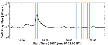
Figure 2: Solar SXR flux on 2007 June 7 in the wavelength range of 0.1 – 0.8 nm. Vertical lines indicate the availability of SOLIS/VSM data.

3.2 Global magnetic energy budget

For all magnetic field configurations, we find that the energy of the extrapolated NLFF field exceeds that of the potential field (i.e., $E_{nlff}>E_{pot}$), both being approximately $10^{25}$ J (see Table 1). This is also the case when considering the evaluated relative error in the energy estimation of about 0.4 % for the potential and 1 % for the NLFF field (i.e. $E_{pot}\leavevmode\nobreak\ \pm$ 0.013 $\times\leavevmode\nobreak\ 10^{25}$ J and $E_{nlff}\leavevmode\nobreak\ \pm$ 0.032 $\times\leavevmode\nobreak\ 10^{25}$ J, respectively). The available free magnetic energy is always approximately $10^{24}$ J with a relative error of about 14 % (i.e. $E_{free}\leavevmode\nobreak\ \pm$ 0.026 $\times\leavevmode\nobreak\ 10^{24}$ J). These uncertainty ranges were checked by comparing similar results for 3D fields during the quiet period, and once by calculating the energy variation in the force-free fields after adding artificial noise to the original magnetograms. Both $E_{pot}$ and $E_{nlff}$ were highest in the phase of increasing emission from the C1.0 flare. During the 20 minute time period of the flare (17:10 UT – 17:29 UT, see Fig. 3) the magnetic energy decreased by $\Delta E_{nlff}=2.01\times 10^{24}$ J, i.e. $\approx$ 38 % of the available free magnetic energy was released. Although the flare was already declining in intensity at 17:29 UT, it still showed a SXR flux of above background B-level (see Fig. 2). The next vector magnetogram snapshot was acquired only 3 hours later at 20:30 UT (see panel (d) of Fig. 1) and the free magnetic energy had decreased further, such that $\approx$ 88.16 % of the original amount of free energy had been released. At 20:30 UT, the magnetic energy was only $\approx$ 0.6 % of the total energy and consequently the magnetic field was almost potential.
From Fig. 2, we can see that AR10960 showed only background B-level activity (i.e. a SXR emission $<$ 10^-7 Wm^-2) at about 18:15 UT and almost the entire free magnetic energy may have been released by that time. Unfortunately, no vector magnetograph data was available immediately after the declining phase of the flare and we are unable to confirm this supposition. For the AR studied here, the maximum excess energy of a NLFF field over the potential field was about 5 % during the investigated period. Since this so-called free energy is an upper limit to the available energy to drive eruptive phenomena, consequently only a small C1.0 flare was recorded. No further flares occurred between 20:30 UT and 21:42 UT for which SOLIS data is available, but five C-class flares were recorded about 3 hours later on 2007 June 8 between 01:00 UT and 16:00 UT. However, a significant amount of free magnetic energy accumulated again during the quiet period after 20:30 UT (see Table 1 and Fig. 3) so that the energy content of the field increased and became, with some fluctuation, comparable to that measured before the C1.0 flare.
From a visual inspection of the magnetic field lines within the extrapolation volume, we recognize some changes in the magnetic field structure during the C1.0 flare (see Fig. 4). We find that the field lines show their highest vertical extent when the C1.0 flare peaked (panel (b)). Ten minutes earlier a comparable field structure was found (panel (a)), but with a lower vertical extend. Nine minutes after the flare peaked, the field line configuration reached its lowest vertical extent (panel (c)), and more field lines of the NLFF field left the extrapolation volume. However, at 20:30 UT, which corresponds to the field configuration of the lowest energy content, the field clearly appears to have restructured, reaching on average its lowest altitude. The return to an almost potential structure could be assigned to a coronal mass ejection (CME) recorded by the SoHO/LASCO instrument on 2007 June 7 around 17:30 UT which could have bodily removed magnetic helicity of the coronal field.

Table 1: Magnetic energy of the extrapolated field.

Time	Magnetic energy $\mathrm{[\leavevmode\nobreak\ \times\leavevmode\nobreak\ 10^{25}\leavevmode\nobreak\ J\leavevmode\nobreak\ ]}$
$\mathrm{(\leavevmode\nobreak\ UT\leavevmode\nobreak\ )}$	$E_{pot}^{(1)}$	$E_{nlff}^{(2)}$	$E_{free}^{(3)}$	$E_{nlff}/E_{pot}^{(4)}$
17:10	3.130	3.282	0.152	1.049
17:20	3.122	3.272	0.149	1.048
17:29	2.986	3.081	0.095	1.032
20:30	3.024	3.042	0.018	1.006
20:39	3.031	3.127	0.095	1.031
21:02	2.969	3.084	0.116	1.039
21:11	2.938	3.028	0.090	1.031
21:33	2.939	3.125	0.185	1.063
21:42	2.933	3.085	0.152	1.052

⁽¹⁾ Energy of the potential and ⁽²⁾ NLFF field, ⁽³⁾ upper limit of the free energy, and ⁽⁴⁾ excess energy of the NLFF over the potential field.

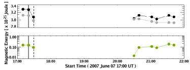
Figure 3: Upper panel: magnetic energy of the potential (gray) and NLFF (black) field. Lower panel: upper limit for the free magnetic energy (shown on logarithmic scale). Solid and dashed lines represent the recorded C1.0 flare and CME, respectively.

4 Discussion

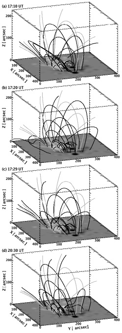
Figure 4: Panels (a), (b), and (c) show the magnetic field configuration during the C1.0 flare. Panel (d) shows the minimum energy configuration. Shown are field lines of the potential (gray) and NLFF (black) field. For improved visibility, the $z$-axis is drawn elongated.

We have investigated the coronal magnetic field associated with the NOAA AR 10960 on 2007 June 7 by analyzing SOLIS/VSM data. Three vector magnetograms with a time cadence of $\approx$ 10 minutes were available to investigate the magnetic energy content of the coronal field during a C1.0 flare, and six further snapshots were acquired to analyze a very quiet time about three hours after the flare. Before as well as after the small flare, the magnetic field energy was $E_{nlff}\approx 3\times 10^{25}$ J. The NLFF field had a free energy of $E_{free}\approx 1.5\times 10^{24}$ J before the flare. As a consequence of the flare/CME, this free magnetic energy reduced by almost a factor of 10 and produced an almost potential configuration. Six snapshots acquired within a time period of about $70$ minutes, during a quiet period of 3 – 4 hours after the flare, showed again an increase in the free magnetic energy. Since the estimated free magnetic energy remained only about 5 % of the total energy content, no large eruption was produced by AR 10960.
This is clearly different from the flaring of AR 10540 observed on 2004 January 18 – 21, which was analyzed in a previous work with the help of vector magnetograph data from the Solar Flare Telescope in Japan of time cadence of about 1 day. In this AR, the free energy was $E_{free}\approx$ 66 % of the total energy, which was sufficiently high to power a M6.1 flare (for details see Thalmann & Wiegelmann, 2008). The activity of AR 10540 investigated earlier was significantly higher than for the data analyzed in the current paper, as was the total magnetic energy. However, despite these differences, we also found some common features. Magnetic energy accumulates before the flare and a significant part of the excess energy is released during the flare. The high amount of free magnetic energy available in AR 10540 produced M-class flares, while the relatively small amount of free energy in AR 10960 powered only a small C-class flare. In both cases, all three components of the vector magnetogram changed during the flare, but the energy decrease in the NLFF field was always higher than that of the potential field, i.e. the energy release was more related to the change in the transverse magnetic field components – which correspond to the field aligned electric currents in the corona – than to that of the longitudinal component.