First-principles methodology for quantum transport in multiterminal junctions

Abstract

We present a generalized approach for computing electron conductance and I-V characteristics in multiterminal junctions from first-principles. Within the framework of Keldysh theory, electron transmission is evaluated employing an O(N) method for electronic-structure calculations. The nonequilibrium Green function for the nonequilibrium electron density of the multiterminal junction is computed self-consistently by solving Poisson equation after applying a realistic bias. We illustrate the suitability of the method on two examples of four-terminal systems, a radialene molecule connected to carbon chains and two crossed carbon chains brought together closer and closer. We describe charge density, potential profile, and transmission of electrons between any two terminals. Finally, we discuss the applicability of this technique to study complex electronic devices.

I Introduction

Electron transport through molecular-scale devices has become a very exciting research area for both experimentalists and theorists. The main reason for this interest originates from the possibility of extreme miniaturization in electronic devices. In recent years, hundreds of papers have been published to establish the connection between the microscopic characteristics of an electronic system, such as the atomic configuration and the electronic structure, and transport properties such as electrical current and conductance. These results have helped to improve the understanding of the I-V characteristics of nanojunctions. However, the interpretation of the I-V curves in terms of the geometry of the junction remains largely a fundamental challenge for molecular electronics. In fact, it has not yet been possible to establish a general theoretical model that can reliably deal with any molecular junction of arbitrary geometry. Owing to the complexity of the system, these studies are strongly dependent on the existence of reliable theoretical treatments based on first-principles approaches. In some instances, even conventional approaches based on density-functional theory (DFT) are expected to break down, especially in the case of weak coupling Koentopp et al. (2008). Nevertheless, DFT is expected to provide reliable results in a large number of cases. To the best of our knowledge, all the existing approaches to date, based on ab initio calculations, can deal with systems limited to two terminals only. It is therefore of widespread interest to develop robust computational schemes that can routinely and reliably account for the transport mechanism in multiterminal molecular devices.

In his seminal work, Büttiker Büttiker (1986) developed a conductance formula for a four-terminal system. However, that formula was not explicitly implemented in the framework of first-principles based calculations. Moreover, since the idea of that paper was to propose a reliable method for voltage difference measurements, Büttiker assumed that only two of the leads can carry current to and from the sample and the two others only measure the voltage. A similar non-atomistic approach based on tight-binding approximation has been presented by Baranger et al. Baranger et al. (1999). Within the framework of a Luttinger liquid theory the four-terminal resistance of an interacting quantum wire was studied by Arrachea et al. Arrachea et al. (2008). Recently, Jayasekera et al. proposed a four-terminal approach for magneto-transport properties based on R-matrix theory Jayasekera et al. (2006). However the approach is only applicable to two-dimensional devices, it is formulated in the framework of semi-empirical tight-binding, and does not include a self-consistent treatment of finite applied potential. Finally, a mesoscopic treatment for phonon-assisted current through multiterminal conductors was formulated by Rychkov et al. Rychkov et al. (2005). While these multiterminal approaches address important issues, they neither treat the system in an ab initio fashion, including atomistic details, nor do they account for the self-consistent (SC) rearrangement of electrons as the bias and the current increase. The importance of the self-consistency had been demonstrated in our previous paper Lu et al. (2005), showing that negative differential resistance in the I-V characteristic can only be quantitatively studied when self-consistency is included.

In this paper, we present a generalized approach for computing conductance and I-V characteristics in multiterminal junctions, based on density-functional theory. In order to take into account the difference in electro-chemical potentials in different leads, we use non-equilibrium Keldysh formalism. The electronic transport is formulated in the basis of an O(N) method for electronic-structure calculations, which is an ab initio pseudopotential density functional approach using a linear combination of numerical atomic orbitals (LCAO) basis that are optimized for the problem in hand Fattebert and Bernholc (2000). We apply external bias voltage through any lead in a realistic way and self-consistently compute the nonequilibrium Green function for the nonequilibrium electron density of the multiterminal junction by solving Poisson equation. One of the main advantages of our scheme is that we can apply bias through any number of leads and at the same time compute current between any two leads. The method is illustrated on two prototypical four-terminal systems (i) a radialene molecule connected to carbon chains, and (ii) two crossed carbon chains brought together closer and closer. We discuss the charge density, potential profile, and transmission of electrons between any two terminals. We also evaluate the current flowing between them. The algorithmic approach has been implemented on massively parallel computer architectures, and can therefore be applied to systems of realistic sizes.

The paper is organized as follows. The basic theory is outlined in section II, sketching a nonequilibrium Green function formulation of the conductance calculations. The applications are discussed in Section III. The scheme is applied to two simple systems, addressing in particular the symmetry in transmission and effect of the different bias voltages on the I-V curves. The paper concludes with a summary in Section IV.

II Theory

In this section, we describe the theoretical aspects of conductance calculations. The general system setup, the coupling to the leads, the equilibrium and nonequilibrium density matrices, the implementation of the bias voltage through any number of leads, and the conductance formula are presented.

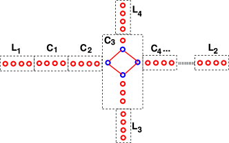
Figure 1: (Color online) Schematic diagram of a multiterminal junction. The barrier region is divided into $n$-number of blocks $\mathsf{C_{1},C_{2},C_{3},\cdots,C_{n}}$ . The leads $\mathsf{L_{1},L_{2}}$ are connected to blocks $\mathsf{C_{1},C_{n}}$, respectively, whereas the remaining leads $\mathsf{L_{3},L_{4}}$ are connected to block $\mathsf{C_{3}}$.

II.1 System setup

We consider the prototypical multiterminal system sketched in Fig. 1. Two or more semi-infinite leads $\mathsf{L_{1},L_{2},L_{3},\ldots}$ are coupled to a central barrier region $\mathsf{C}$ with thermal reservoirs that are maintained at the electro-chemical potentials $\mathsf{\mu_{1},\mu_{2},\mu_{3},\cdots}$. Within our approach, region $\mathsf{C}$ can be treated as $n$ subregions as $\mathsf{C_{1},C_{2},C_{3},\ldots,C_{n}}$ and, in principle, we may connect $m$-number of leads to them. Note that an important hypothesis of the approach (also implicit in all two-terminal approaches based on Green function) is that there are no direct interactions between the leads and they only interact via the barrier region. Consequently the overlap integrals between orbitals on atoms situated in different leads take place via the barrier region only.

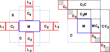
Figure 2: (Color online) (Left) Schematic of a four-terminal system. The leads $\mathsf{L_{1},L_{2},L_{3}}$ and $\mathsf{L_{4}}$ are connected to the molecular barrier $\mathsf{M}$ via the subregions $\mathsf{C_{1},C_{2},C_{3}}$, and $\mathsf{C_{4}}$ respectively. The subregions $\mathsf{C_{3},C_{4}}$ and the molecular region $\mathsf{M}$ are considered together as a single region $\mathsf{C}$ shown by the blue-dotted box. The black-dotted box shows the extended-scattering region $\mathsf{S}$. (Right) Tri-diagonal matrix representation of this system. Any matrix-element in the lower off-diagonal-blocks is the complex conjugate of the corresponding element in the upper off-diagonal-blocks and therefore one can avoid storing the lower off-diagonal-blocks. The shaded blocks of the matrix are directly connected to the leads and hence these contain the same matrix-elements as in the respective leads.

For reasons of simplicity, we will be discussing a four-terminal system as an example. However, the method can be readily generalized to any number of electrodes. Suppose the leads $\mathsf{L_{1},L_{2},L_{3}}$ and $\mathsf{L_{4}}$ are connected to the molecular barrier $\mathsf{M}$ via the subregions $\mathsf{C_{1},C_{2},C_{3}}$ and $\mathsf{C_{4}}$ respectively. At the beginning of the calculation, each subregion has the same potential and charge distribution as its respective connected lead.

In order to study the transport properties, in principle, we need to invert an infinite Hamiltonian of the infinite system which includes all parts of the semi-infinite leads. However, the electrons injected from the reservoirs move ballistically through the leads and all scattering events only occur around the barrier region (molecular region), called extended-scattering region $\mathsf{S}$ [see Fig. 2 (left)]. The potential is modified only within a finite region of the leads, the one being connected to the barrier region. It is therefore sufficient to consider a finite Hamiltonian containing all subregions $\mathsf{C_{1},C_{2},C_{3},C_{4}}$ and the barrier region $\mathsf{M}$. The Hamiltonian matrix of this system is of finite rank and takes the form

$$\begin{pmatrix}H_{\mathsf{C_{1}}}+\Sigma_{\mathsf{\mu_{1}}}&0&V_{\mathsf{C_{1}M}}&0&0\\ 0&H_{\mathsf{C_{3}}}+\Sigma_{\mathsf{\mu_{3}}}&V_{\mathsf{C_{3}M}}&0&0\\ V_{\mathsf{MC_{1}}}&V_{\mathsf{MC_{3}}}&H_{\mathsf{M}}&V_{\mathsf{MC_{4}}}&V_{\mathsf{MC_{2}}}\\ 0&0&V_{\mathsf{C_{4}M}}&H_{\mathsf{C_{4}}}+\Sigma_{\mathsf{\mu_{4}}}&0\\ 0&0&V_{\mathsf{C_{2}M}}&0&H_{\mathsf{C_{2}}}+\Sigma_{\mathsf{\mu_{2}}}\end{pmatrix},$$ (1)

where $H_{\mathsf{C}_{i}},H_{\mathsf{M}}$ are the Hamiltonian matrices in the $i$th-lead and the molecular barrier respectively, and $V_{\mathsf{C}_{i}\mathsf{M}}$ is the interaction between the $i$th-lead and the barrier $\mathsf{M}$. $\Sigma_{\mathsf{\mu}}$’s are the self-energies that couple the scattering region to the remaining parts of the semi-infinite leads. The Hamiltonian and the charge density matrix are assumed to be converged to the bulk values in the leads outside the scattering region. For practical calculations, this assumption is tested by including larger fractions of the leads in the scattering region and by examining the charge convergence during the SC iterations. Here the term “charge convergence” refers to the conservation of total charge in the scattering region. The charge convergence criterion is of crucial importance, since a failure to fulfill it would indicate bad numerical convergence or issues with the setup of the size of the extended region. By achieving the charge convergence, we make sure that all the screening takes place within the scattering region.

The Hamiltonian matrix in Eq. 1 can be written explicitly in a tri-diagonal form, as explained below. Consider the subregions $\mathsf{C_{3},C_{4}}$ and the region $\mathsf{M}$ as a single region $\mathsf{C}$, schematically shown in Fig. 2. One can rewrite the above Hamiltonian matrix as:

$$\begin{pmatrix}H_{\mathsf{C_{1}}}+\Sigma_{\mathsf{\mu_{1}}}&V_{\mathsf{C_{1}C}}&0\\ V_{\mathsf{CC_{1}}}&H_{\mathsf{C}}&V_{\mathsf{CC_{2}}}\\ 0&V_{\mathsf{C_{2}C}}&H_{\mathsf{C_{2}}}+\Sigma_{\mathsf{\mu_{2}}}\end{pmatrix},$$ (2)

where

$$H_{\mathsf{C}}=\begin{pmatrix}H_{\mathsf{C_{3}}}+\Sigma_{\mathsf{\mu_{3}}}&V_{\mathsf{C_{3}M}}&0\\ V_{\mathsf{MC_{3}}}&H_{\mathsf{M}}&V_{\mathsf{MC_{4}}}\\ 0&V_{\mathsf{C_{4}M}}&H_{\mathsf{C_{4}}}+\Sigma_{\mathsf{\mu_{4}}}\end{pmatrix},$$

We proceed with the above tri-diagonal Hamiltonian for multiterminal calculations in the same way as in a two-terminal case.Brandbyge et al. (2002) The most time-consuming part is the calculation of the Green functions, i.e., the inversion of a matrix $(\epsilon S-H)$, where H is the Hamiltonian matrix in Eq. 1 and S is the overlap matrix. For a large system, the matrix can be further reduced to a tri-diagonal matrix with smaller blocks. Its inversion can be done by an iterative method. It can also be efficiently carried out using sparse algebra. In fact, the numerical effort to invert the matrix is independent of the number of terminals. The matrix size (or the system size) and its sparsity play an important role in determining the computational cost.

II.2 Density Matrix

In this subsection, we first outline the procedure adopted for computing the density matrix for a two-terminal system Brandbyge et al. (2002); Thygesen et al. (2003); Buongiorno Nardelli (1999) and then generalize it for a multiterminal system.

As explained in detail in Ref. Brandbyge et al., 2002 for a two-terminal system, one may write the density matrix as

$$\boldsymbol{D}_{\nu\nu^{\prime}}=\int_{-\infty}^{\infty}d\epsilon\left[\rho_{\nu\nu^{\prime}}^{\mathsf{L_{1}}}(\epsilon)\,n_{F}(\epsilon-\mathsf{\mu_{1}})+\rho_{\nu\nu^{\prime}}^{\mathsf{L_{2}}}(\epsilon)\,n_{F}(\epsilon-\mathsf{\mu_{2}})\right],$$ (3)

$$\rho_{\nu\nu^{\prime}}^{\mathsf{L}_{i}}(\epsilon)=\frac{1}{\pi}\left[\mathrm{G}(\epsilon)\,\Gamma_{\mathsf{L}_{i}}(\epsilon)\,\mathrm{G}^{\dagger}(\epsilon)\right]_{\nu\nu^{\prime}},i=1,2$$ (4)

where $\nu$ and $\nu^{\prime}$ are the indexes of localized orbitals in the extended scattering region, ${\mathrm{G}}$ the Green function, and $\Gamma_{\mathsf{L}_{i}}(\epsilon)=i\left[\Sigma_{\mathsf{L}_{i}}(\epsilon)-\Sigma_{\mathsf{L}_{i}}(\epsilon)^{\dagger}\right]/2$ is the coupling function for the $i$th-lead. $\Sigma_{\mathsf{L}_{i}}(\epsilon)=\left[V\,g^{i}(\epsilon)\,V^{\dagger}\right]$ is the self-energy of the $i$th-lead that couples it to the extended-scattering region.

The density matrix given in Eq. 3 is general, i. e., it is valid for both equilibrium or nonequilibrium electron transport. It can be separated into two parts

$$\boldsymbol{D}_{\nu\nu^{\prime}} = -\frac{1}{\pi}\,\mbox{Im}\left[\int^{\infty}_{\mbox{EB}}d\epsilon\,\mathrm{G}(\epsilon+i\delta)\,n_{F}(\epsilon-\mathsf{\mu_{1}})\right]$$ (5)

$$+ \int_{-\infty}^{\infty}d\epsilon\,\rho_{\nu\nu^{\prime}}^{\mathsf{L_{2}}}(\epsilon)\,\left(n_{F}(\epsilon-\mathsf{\mu_{2}})-n_{F}(\epsilon-\mathsf{\mu_{1}})\right).$$

where EB is the low energy bound for the valence band. The first and second parts contain the equilibrium and nonequilibrium density matrices, respectively.

II.3 Generalized density matrix for multiterminal junction

Equation 5 is now generalized to the general multiterminal case. The generalized density matrix is now

$$\boldsymbol{D}_{\nu\nu^{\prime}} = \sum_{i}\int_{-\infty}^{\infty}d\epsilon\,\rho_{\nu\nu^{\prime}}^{\mathsf{L}_{i}}(\epsilon)\,n_{F}(\epsilon-{\mathsf{\mu}_{i}})$$

$$= \int_{-\infty}^{\infty}d\epsilon\,\rho_{\nu\nu^{\prime}}^{\mathsf{L}_{m}}(\epsilon)\,n_{F}(\epsilon-{\mathsf{\mu}_{m}})+\sum_{j\neq m}\int_{-\infty}^{\infty}d\epsilon\,\rho_{\nu\nu^{\prime}}^{\mathsf{L}_{j}}(\epsilon)\,n_{F}(\epsilon-\mathsf{\mu}_{j})$$

$$= \int_{-\infty}^{\infty}d\epsilon\,\left(\sum_{i}\rho_{\nu\nu^{\prime}}^{\mathsf{L}_{i}}(\epsilon)\right)\,n_{F}(\epsilon-{\mathsf{\mu}_{m}})+\sum_{j\neq m}\int_{-\infty}^{\infty}d\epsilon\,\rho_{\nu\nu^{\prime}}^{\mathsf{L}_{j}}(\epsilon)\,n_{F}(\epsilon-\mathsf{\mu}_{j})-\sum_{j\neq m}\int_{-\infty}^{\infty}d\epsilon\,\rho_{\nu\nu^{\prime}}^{\mathsf{L}_{j}}(\epsilon)\,n_{F}(\epsilon-{\mathsf{\mu}_{m}})$$

$$= -\frac{1}{\pi}\,\mbox{Im}\left[\int^{\infty}_{\mbox{EB}}d\epsilon\,\mathrm{G}(\epsilon+i\delta)\,n_{F}(\epsilon-{\mathsf{\mu}_{m}})\right]+\sum_{j\neq m}\int_{-\infty}^{\infty}d\epsilon\,\rho_{\nu\nu^{\prime}}^{\mathsf{L}_{j}}(\epsilon)\left[n_{F}(\epsilon-\mathsf{\mu}_{j})-n_{F}(\epsilon-{\mathsf{\mu}_{m}})\right],$$

where energy EB is chosen to be low enough to include all of the valence bands and $\mu_{m}$ is the electro-chemical potential of the $m$th-lead. In practice, each $D_{\nu\nu^{\prime}}$ is calculated separately for each $\mu_{m}$ being equal to the chemical potential of a given lead $m$. All $D_{\nu\nu^{\prime}}$ to reduce the numerical error related to the integration.

For $\mu_{m}=\mu_{i}$, the electro-chemical potential of the lead $i$, the density matrix is

$$\boldsymbol{\tilde{D}}_{\nu\nu^{\prime}}^{i}=\boldsymbol{D}_{\nu\nu^{\prime}}^{i}+\sum_{j\neq i}\Delta_{\nu\nu^{\prime}}^{ij}$$ (6)

where

$$\boldsymbol{D}_{\nu\nu^{\prime}}^{i}=-\frac{1}{\pi}\,\mbox{Im}\left[\int^{\infty}_{\mbox{EB}}d\epsilon\,\mathrm{G}(\epsilon+i\delta)\,n_{F}(\epsilon-\mathsf{\mu}_{i})\right]$$

$$\boldsymbol{\Delta}_{\nu\nu^{\prime}}^{ij}=\int_{-\infty}^{\infty}d\epsilon\,\rho_{\nu\nu^{\prime}}^{\mathsf{L}_{j}}(\epsilon)\left[n_{F}(\epsilon-\mathsf{\mu}_{j})-n_{F}(\epsilon-\mathsf{\mu}_{i})\right].$$

$\boldsymbol{D}_{\nu\nu^{\prime}}^{i}$ and $\boldsymbol{\Delta}_{\nu\nu^{\prime}}^{ij}$ are the equilibrium and nonequilibrium parts of the density matrix, respectively. The integral in the first part of Eq. (6) can be carried out with complex contour integral technique as in Ref. Brandbyge et al., 2002. However, the integral in the second part, $\boldsymbol{\Delta}_{\nu\nu^{\prime}}^{ij}$, must be calculated on the real energy axis with a very dense mesh.

Because of errors related to numerical integration, the computed solutions of Eq. (6) will not produce exactly the same results for all $i$’s. So, in order to minimize the error in the solutions, we compute the density matrix as a weighted sum of $\boldsymbol{\tilde{D}}_{\nu\nu^{\prime}}^{i}$ in the following way:

$$\boldsymbol{D}_{\nu\nu^{\prime}}=\sum_{i}w_{\nu\nu^{\prime}}^{i}\boldsymbol{\tilde{D}}_{\nu\nu^{\prime}}^{i},$$ (7)

where

$$w_{\nu\nu^{\prime}}^{i}=\sum_{j\neq i}\sum_{k\neq j}{\left(\Delta_{\nu\nu^{\prime}}^{jk}\right)^{2}}/{\Delta}$$

$$\mbox{and}\ \ \Delta=({\mbox{N}-1})\sum_{i}\sum_{j\neq i}\left(\Delta_{\nu\nu^{\prime}}^{ij}\right)^{2},$$

which satisfies $\sum_{i}w_{\nu\nu^{\prime}}^{i}=1$, with N being the number of leads. The weight $w_{\nu\nu^{\prime}}^{i}$ is chosen to minimize the numerical error in the solution.Brandbyge et al. (2002) We test the convergence by increasing the density of the energy mesh, thereby making sure that the integration yields accurate final results.

II.4 Computation of the conductance

We apply Keldysh theory for the computation of the conductance of the multiterminal junction. Within the ‘electron counting’ picture of transport, the conductance $G$ of the junction is obtained from the transmission probabilities of all scattering channels entering from one lead and leaving through the other,Imry and Landauer (1999)

$$G(V)=G_{0}\,T(V),$$

where $V$ is the applied bias voltage. The conductance quantum $G_{0}=e^{2}/h$ is the inverse von-Klitzing constant (i. e. the quantum of resistance, $R_{\mathrm{K}}\approx 25.8\,\mathrm{k\Omega}$). The total transmittance $T(V)$ comprises the transmission probabilities in the ‘energy window of tunneling’ opened by $V$.Henk and Bruno (2003)

Once the potential profile is self-consistently determined, the transmission spectrum from leads ${\mathsf{L}_{i}}$ to ${\mathsf{L}_{j}}$ under the external applied bias, $V=\mathsf{\mu}_{i}-\mathsf{\mu}_{j}$, can be calculated as

$$T_{\mathsf{L}_{ij}}(\epsilon,V)=\frac{2e^{2}}{h}\mbox{Tr}\left[\Gamma_{\mathsf{L}_{i}}(\epsilon)\,\mathrm{G}^{+}(\epsilon)\,\Gamma_{\mathsf{L}_{j}}\,\mathrm{G}^{-}(\epsilon)\right],$$ (8)

with

$$\Gamma_{\mathsf{L}_{i}}=i\left[\Sigma_{\mathsf{L}_{i}}^{\mathsf{C}_{i}\mathsf{C}_{i}}-{\Sigma_{\mathsf{L}_{i}}^{\mathsf{C}_{i}\mathsf{C}_{i}}}^{\dagger}\right]\!/2,\ \Sigma_{\mathsf{L}_{i}}^{\mathsf{C}_{i}\mathsf{C}_{i}}=V_{\mathsf{C}_{i}\mathsf{L}_{i}}\;g_{\mathsf{L}_{i}}\;V^{\dagger}_{\mathsf{C}_{i}\mathsf{L}_{i}},$$

where $\mathrm{G}^{\pm}$ are the advanced and retarded Green functions for the extended-scattering region $\mathsf{S}$, and $g_{\mathsf{L}_{i}}$ is the surface Green function of the $i$th-lead.

The current from the lead $\mathsf{L}_{i}$ to $\mathsf{L}_{j}$ through the molecular barrier is given by

$$I_{\mathsf{L}_{ij}}(V)=\int_{-\infty}^{\infty}T_{\mathsf{L}_{ij}}(\epsilon,V)\left[f(\epsilon-{\mathsf{\mu}_{i}})-f(\epsilon-\mathsf{\mu}_{j})\right]d\epsilon,$$

where $f$ is the Fermi-Dirac distribution.

Although the present multiterminal NEGF approach was derived and carried out only within DFT, it can serve as a starting point for implementation of many-body corrections at the quasi-particle Hedin (1965); Hybertsen and Louie (1988) or self-interaction correction Perdew and Zunger (1981); Toher and Sanvito (2007) levels. A time-dependent formulation Kurth et al. (2005) is also possible.

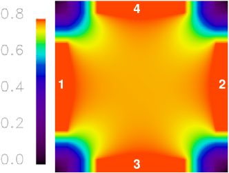
Figure 3: An initial bias profile (size 60 Bohr $\times$ 60 Bohr) for a four-terminal junction to be applied to the system at the beginning of a nonequilibrium calculation. For the planar molecules considered here, it has been generated by solving a 2D Laplace’s equation with appropriate boundary conditions (see text for details). An identical bias voltage $0.8\,V$ is applied through all four leads $\mathsf{L_{1},L_{2},L_{3}}$ and $\mathsf{L_{4}}$. The leads are denoted by the numbers 1, 2, 3, 4, respectively, and the scale bar of the potential is in eV.

II.5 Finite bias

In a two-terminal system, the initial potential for an applied bias can be simply a linear interpolation independent of the bias between the electrodes. The situation is not as simple in three or four terminal system. First, one needs to make sure that the potentials of all electrodes (outside the extended-scattering region $\mathsf{S}$) will be unaffected by the applied bias voltage, in other words, the modified potential has to match at the boundary of each electrode and the region $\mathsf{S}$. Second, the variation of the potential between any two electrodes through the molecular barrier has to be continuous and uniform. Third, the electrostatic potential in the vacuum region between two arbitrary electrodes has to be realistic. In order to create such an initial profile for the planar molecules considered here, we iteratively solve the 2D Laplace’s equation (assuming the system is in the xy-plane) in a hypothetical system where the extended scattering region is empty:

$$\frac{\partial^{2}V(x,y,z)}{\partial x^{2}}+\frac{\partial^{2}V(x,y,z)}{\partial y^{2}}=0,$$

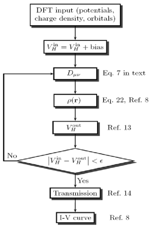
Figure 4: Flowchart of the self-consistent loop used to calculate I-V characteristics. The terminology is explained in the text.

with the following boundary conditions: (a) the initial potential in the scattering region is zero (or may be the same as the potentials of the four leads), (b) the potential in every lead is unchanged, (c) the potential towards the vacuum region, that is, at the corners of the box, decays.

Solving Laplace equation yields an initial bias-potential profile, as shown in Fig. (3), for a given xy-plane of the system. In the simple of planar molecules, we repeat this image for the other planes of the 3D system. In more complex cases, a 3D solution of an approximate initial value problem would be used. We stress that the solution of Laplace equation is merely a starting guess of the bias potential that is being updated via the SC calculation. During the course of our implementation and testing, we found that using this solution in the first iteration significantly accelerates the convergence. It is a very effective guess to initiating the SC iterations, as the solution to Laplace equation is the correct one for the given setup in absence of the central part. Once the potential, charge density, etc. are converged, the final result is independent of the initial guess.

II.6 Computational Details

The electronic properties of the tunnel junctions discussed in Section III are obtained within the nonequilibrium Green function (NEGF) approach Larade et al. (2001); Brandbyge et al. (2002) using a basis of optimally localized orbitals, Fattebert and Bernholc (2000); Buongiorno Nardelli et al. (2001) and a multi-grid approach. The ab initio calculations for the leads and the molecule are performed with the O(N) method, details of which can be found in Ref. Fattebert and Bernholc, 2000. The exchange and correlation terms are represented in the generalized gradient approximation (GGA). Perdew et al. (1996) The electron-ion interactions are described by nonlocal, ultrasoft pseudopotentials. Vanderbilt (1990) The surface Green functions are calculated with a transfer-matrix technique in an iterative scheme. Sancho et al. (1985) The potential and charge density in the leads are fixed to those corresponding in the bulk material. The central conductor part includes enough “buffer layers” of the lead so that the potential and the charge density match at the interfaces between the conductor and leads after the SC calculations. The Hartree potential is obtained by solving Poisson equation with boundary conditions matching the electrostatic potentials of all the leads. The generated SC potentials and charge density serve as inputs for the conductance calculations. The flowchart in Fig. (4) explains the relations between the various steps in our algorithm. The computations use a massively parallel real-space multigrid implementation Briggs et al. (1996) of density-functional theory DFT. Kohn and Sham (1965) The wave functions and localized orbitals are represented on a grid with spacing of 0.335 Bohr. A double grid technique Ono and Hirose (1999) is employed to evaluate the inner products between the nonlocal potentials and the wave functions, thereby substantially reducing the computational cost and memory without loss of accuracy.

II.7 Parallelization on Supercomputers

We now describe our multi-level parallel implementation of the multiterminal transport theory outlined above. First, the matrices are distributed according to the two-dimensional block-cyclic data layout scheme used by ScaLAPACK. Depending on the matrix size, one can use $n\times n$ processors for matrix operations (typically n = 1 to 4 in our applications). Second, parallelization proceeds over the energy points used in the integration to obtain the charge density matrix. Third, potentials and density matrices are also parallelized over the 3D processor grid $pe_{x},pe_{y},pe_{z}$, where $pe_{x}\times pe_{y}\times pe_{z}$ is the total number of processors. This step of parallelization drastically accelerates the Poisson equation solver during the self-consistent iterations. Fourth, parallelization over the bias points is trivial and can be achieved with nearly 100% efficiency.

For the zero bias calculation, the computational cost for a multiterminal system is about the same as that for a two-terminal system if the number of atoms in the scattering region is the same. However, for the multiterminal system, an additional computational time is required for the nonequilibrium calculation. This is because, as the number of leads increases, the number of terms in the density matrix also increases (see in Eq. 6). The most time-consuming part of the entire computation is the matrix inversion needs to calculate the Green functions. This part scales nearly linearly if one takes into consideration the sparsity feature of the Hamiltonian and overlap matrices.

III Applications

III.1 Radialene molecule

In order to illustrate the proposed approach for calculating the conductance of a multiterminal molecular device, we choose a four-terminal junction of radialene molecule connected to semi-infinite carbon chains as a first example. A schematic diagram is shown in the inset of Fig. 5. The system has C_4v symmetry. Applying our technique to this system, we expect to see the same symmetry in the converged potential profile, which should also be reflected in the transmission curves.

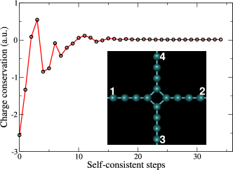
Figure 5: (Color online) Charge convergence of the radialene system with SC steps at zero bias. In the inset, a schematic view of the central region of the four-terminal radialene junction is shown, with the number 1, 2, 3 and 4 marking the positions of the leads. The size of the system is 60 Bohr $\times$ 60 Bohr.

Our nonequilibrium Green function (NEGF) technique Larade et al. (2001); Brandbyge et al. (2002) uses a basis of optimal localized orbitals. Fattebert and Bernholc (2000); Buongiorno Nardelli et al. (2001) The atom-centered orbitals are optimized variationally in the equilibrium geometry. In the radialene based system, we include 48 atoms in the calculation and each atom has six orbitals with the radii of 9 Bohr. A self-consistent calculation is carried out within an extended zone around the scattering region. For this system, the total charge is converged after 18 steps of the SC process, as shown in Fig. 5. The charge density determines the potential.

Fig. 6 (left) shows the converged potential profile at zero bias 4.88 Bohr above the atomic plane. The C_4v symmetry of the system is reflected in its potential profile. After the convergence of the charge density is achieved for the equilibrium density matrix, we apply the bias voltage through the leads. At this stage, the nonequilibrium part of the density matrix (see Eq. 6) is included through an iterative process. In Fig. 6 (right) we show the converged potential profile after applying an identical bias of $0.8\,V$ through all the leads. It again shows the four-fold symmetry as expected. It also shows that after the convergence, the potential matches very well at the boundary of the leads and the central molecule.

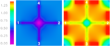
Figure 6: (Color online) (Left) Self-consistent converged potential profile (same as system size, i.e., 60 Bohr $\times$ 60 Bohr) at zero bias of the four-terminal radialene system, plotted 4.88 Bohr above the atomic plane. (Right) The converged potential profile after applying an identical bias at $0.8\,V$ through all the leads. Both the images are shown in same color scale (in eV), to compare the relative heights of the potentials.

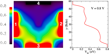
Figure 7: (Color online) (Left) Converged potential profile of the radialene system with a non-uniform bias voltage. (The color scale is in eV.) An identical bias of $0.8\,V$ is applied through three of the leads (denoted by 1, 2, 3) and no bias is applied through the fourth lead. (Right) Potential drop along the central line between the leads 3 and 4.

We now examine the potential drop when different biases through the leads are applied. Here, a bias of $0.8\,V$ is applied at the leads $\mathsf{L_{1},L_{2},L_{3}}$, while the fourth lead $\mathsf{L_{4}}$ is at zero bias. After solving the Poisson equation, we observe a uniform potential drop between the leads $\mathsf{L_{3}}$ and $\mathsf{L_{4}}$ (see Fig. 7 (left)). For testing purposes, we have also plotted the Hartree potential $V_{H}$ along the line connecting leads $\mathsf{L_{3}}$ and $\mathsf{L_{4}}$ in Fig. 7 (right).

Once the potential profile is self-consistently determined, the transmission spectrum under the applied bias $V$ is calculated using the Eq. 8. The transmission curves, shown in Fig. 8, are computed for several bias voltages, with the voltages being the same at $\mathsf{L}_{1},\mathsf{L}_{2}$ and $\mathsf{L}_{3}$, while $\mathsf{L}_{4}$ is being kept at $V=0$. The left and right panels in Fig. 8 show the transmission $\mathsf{L}_{34}$ and $\mathsf{L}_{14}$, respectively. The carbon-atoms in the lead are fixed at equidistant bond length. It follows that the lead has metallic character and therefore no gap appears in the transmission curve (as would be the case if the chain had been subjected to a Jahn-Teller distortion). With zero bias, the transmission curve around the Fermi level is almost constant. This nature of transmission is expected because the free-electron-like $sp$-states of carbon contribute to the transmission. However, with increasing bias, the transmission curve starts to oscillate. The origin of the oscillation is related to the choice of electrode. Here we used a simple, very idealized carbon chain made up of 8 atoms per lead. In order to examine the charge convergence in the scattering region, one needs to define a potential box around the molecule, where the Poisson equation is solved. However, because of the small number of carbon atoms in the lead, the potential box needs to be quite large, encompassing major parts of the leads. This creates finite-size effects, which are reflected in the transmissions showing oscillations. As the bias is increased, the finite size effects also increase and this is why there are more oscillations in the transmission curves with higher bias. Therefore, the these oscillations are an artifact of the small number of atoms in our “test” leads. However, realistic molecular systems, with either thicker nanowires or bulk surfaces, do not show these artifacts. Our investigations of two-terminal systems Lu et al. (2005); Wang et al. (2006); Ribeiro et al. (2008) further demonstrate this claim. In addition, our ongoing investigations on more realistic four-terminal molecular junctions (to be communicated soon) are free of such oscillations.

Note that because of the C_4v symmetry of the system, the transmissions $\mathsf{L_{12}}$ and $\mathsf{L_{34}}$ at zero bias are identical (not shown in the figure). For the same reason, the transmission contributions $\mathsf{L_{13}}$, $\mathsf{L_{14}}$, $\mathsf{L_{23}}$ and $\mathsf{L_{24}}$ are equivalent (not shown in figure).

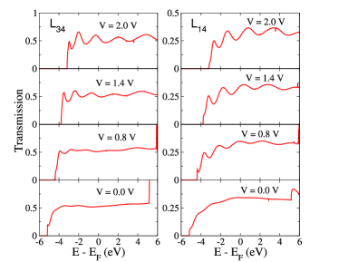
Figure 8: (Color online) Transmission curves of the four-terminal radialene system with different bias voltages. The $E_{F}$ is the Fermi energy of the lead 4. The bias geometry is the same as in Fig. 7. The left and right panels show transmission through the leads $\mathsf{L}_{34}$ and $\mathsf{L}_{14}$, respectively.

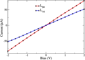
Figure 9: (Color online) Current-voltage characteristics of the four-terminal radialene junction. The bias geometry is as shown in Fig. 7. The current contributions through the leads $\mathsf{L}_{34}$, $\mathsf{L}_{14}$ are displayed.

We have also computed the I-V curves for this system, see Fig. 9. The current contributions through leads $\mathsf{L_{34}}$ (red line) and $\mathsf{L_{14}}$ (blue line) are obtained in the voltage window $\pm 2\,V$. Both curves are increasing almost linearly because of the constant transmission around the Fermi energy.

III.2 Crossed carbon chains

As a second example, we have chosen a four-terminal system consisting of two crossed carbon chains. Our objective is to vertically bring the carbon chains closer and closer, and to see how the current varies with the distance between the chains, possibly leading to a crossover from low to high coupling. In our study, we consider three distances between the chains, $d=$ 7.5, 5.0 and 2.5 Bohr. To build the system, we include a total of 66 carbon atoms, with 33 atoms in each chain. Every atom has 6 basis orbitals with the radius of 9 Bohr, as in previous example. A schematic diagram of the system is shown in Fig. 10.

After the charge convergence is achieved, we apply a $0.5\,V$ bias through leads $\mathsf{L_{1},L_{2},L_{3}}$ and a $-0.5\,V$ bias through the fourth lead $\mathsf{L_{4}}$. The converged potential and the charge density of the equilibrium system (i. e., at zero bias) is used as the initial guess for the convergence of the new nonequilibrium system. Fig. 11 (left-top and bottom) shows the converged potential profiles of the system when the distances between the two carbon chains are 7.5 and 5.0 Bohr, respectively. The plotting plane is parallel to the chains and passes through one of them. Both figures are symmetric about the line connecting leads $\mathsf{L_{3}}$ and $\mathsf{L_{4}}$. To observe the potential drop along this line more clearly, we plot the Hartree potentials as shown in Fig. 11 [(b) and (d)]. If the two chains are sufficiently away from each other, e. g., separated by 7.5 Bohr, the potential drop between two leads is smooth, and thus electron tunneling along a given chain will be the largest in this case. As we bring the chains closer, e. g., to a distance of 5.0 Bohr, the probability for an electron to tunnel from one chain to the other increases significantly.

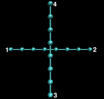
Figure 10: (Color online) A schematic diagram of the crossed-carbon-chains system. Three cases are considered, with distances between the chains of 7.5, 5.0 and 2.5 Bohr.

Fig. 12 shows the transmission curves in all three cases computed through leads $\mathsf{L_{34}}$ (left panel) and $\mathsf{L_{14}}$ (right panel) with zero and non-zero biases. We applied the same bias as in Fig. 11. The transmission of a system consisting of a single ideal lead must be equal to the number of scattering channels at the energy $E$.Henk et al. (2006); Saha et al. (2008) If the carbon chains are far away from each another, e. g., at a distance of 7.5 Bohr, the overlap integral between orbitals on atoms situated in two different leads is close to zero. Therefore, each lead in the system will tunnel current as an isolated electrode. This is why we observe a constant transmission through $\mathsf{L_{34}}$, while the transmission through $\mathsf{L_{14}}$ is almost zero, as expected. In a carbon chain system, a two-fold degenerate band crosses the Fermi level. Consequently, there are two scattering channels and $G=2$. As we decrease the distance between the chains, to 5.0 and 2.5 Bohr, the orbital overlaps between the chains become larger and larger. This results in a decrease in transmission $\mathsf{L_{34}}$ and increase for $\mathsf{L_{14}}$. The total transmission that would occur only through $\mathsf{L}_{34}$ in the bare lead case, is now partially distributed to the other channels. At a finite bias, the transmission curves start to oscillate. As explained in the Subsection III.1, these oscillations are due to electrons that are attracted to the central region, thereby conserving the static charge and creating an “electron-in-a-box” effect with corresponding standing-wave-like oscillations.

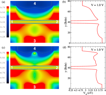
Figure 11: (Color online) (a) and (c) Comparison of the converged potential profiles of the crossed-carbon-chains system when the distances between the two carbon chains are 7.5 and 5.0 Bohr. In both the cases, we apply same bias $0.5\,V$ through the leads $\mathsf{L_{1},L_{2}}$, and ${L_{3}}$ and bias $-0.5\,V$ through the fourth lead $\mathsf{L_{4}}$. The plotting passing through one of the chains. (b) and (d) Potential drops between the leads $\mathsf{L_{3}}$ to $\mathsf{L_{4}}$ for (a) and (c) case.

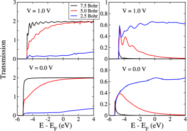
Figure 12: (Color online) Comparison of transmission curves in all three cases, where the distances between the chains are 7.5, 5.0 and 2.5 Bohr, of the crossed-carbon-chain system with zero and non-zero biases (as in Fig. 11). The left and right panels show transmission through leads $\mathsf{L_{34}}$ and $\mathsf{L_{14}}$, respectively.

Fig. 13 shows the flow of current through the channels $\mathsf{L_{34}}$ (left panel) and $\mathsf{L_{14}}$ (right panel). We apply bias $V/2$ through the leads $\mathsf{L_{1},L_{2},L_{3}}$ and bias $-V/2$ through $\mathsf{L_{4}}$, and compute the current for distances 7.5, 5.0 and 2.5 Bohr between the carbon chains. In all cases, as the bias increases, the current increases almost linearly. However, the nonlinearity is expected to be larger in a semiconducting system. It should be noticed that the current contribution through the $\mathsf{L_{34}}$ channel increases with an increase of the distance between the chains, while the current flow through the $\mathsf{L_{14}}$ channel decreases. Note that the currents through the $\mathsf{L_{14}}$ and $\mathsf{L_{24}}$ channels are identical because of the symmetry of the system. It is interesting to see how the current flow through a given channel, say $\mathsf{L_{14}}$, decays while moving the chains away from each other. We have fitted the current contributions at a bias of $1.2\,V$ as $I(d)=I_{0}\ e^{-\beta d}$ and found the exponential decay constant $\beta$ to be 0.97 Bohr^-1.

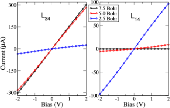
Figure 13: (Color online) Comparison of I-V curves with varying distances between the chains of the crossed-carbon-chain system. The left and right panels show the current contributions through leads $\mathsf{L_{34}}$ and $\mathsf{L_{14}}$, respectively, with the bias voltage.

IV Summary and Conclusions

A new generalized approach for computing nonequilibrium quantum transport in multiterminal systems from first principles is developed within the framework of Keldysh theory. This advance opens up new opportunities to study and design molecule-based electronic devices. All calculations are performed at the density functional theory level with full self-consistency under applied bias. For computational efficiency, we use a compact atom-centered optimized orbitals obtained with a linear scaling method (N is the number of electrons) for computing the electronic properties of the lead and the central region. This basis is used to expand the Green functions, the transmission function, and the charge density under bias, which are self-consistently determined via contour integration. The methodology is developed to scale well on massively-parallel computers, and should therefore be applicable to systems of realistic sizes.

To demonstrate the suitability of the new technique for studying electron transport in multiterminal junctions, we have chosen two very simple four-terminal systems as test applications. In the first example, a radialene system having $C_{4v}$ symmetry is used to test the conservation of symmetry and the numerical robustness of our implementation. In the second example, we have examined the conductance properties of two crossed carbon chains. The I-V characteristics of the chains show the expected trends with the changing strength of interactions. These demonstrations establish the general applicability of the method. Since our code is efficient and highly parallel, we are able to deal with rather large systems. One such application (a four-terminal system consisting of an organic molecule [9,10-Bis(($2^{\prime}$-para-mercaptophenyl)-ethinyl)-anthracene] connected to four gold nanowires) will be published elsewhereSaha et al. (2009).

References

- Koentopp et al. (2008) M. Koentopp, C. Chang, K. Burke, and R. Car, J. Phys.: Condens. Matt. 20, 083203 (2008).
- Büttiker (1986) M. Büttiker, Phys. Rev. Lett. 57, 1761 (1986).
- Baranger et al. (1999) H. U. Baranger, D. P. DiVincenzo, R. A. Jalabert, and A. D. Stone, Phys. Rev. B 44, 10637 (1999).
- Arrachea et al. (2008) L. Arrachea, C. Na’on, and M. Salvay, Phys. Rev. B 77, 233105 (2008).
- Jayasekera et al. (2006) T. Jayasekera, J. A. Morrison, and K. Mullen, Phys. Rev. B 74, 235308 (2006).
- Rychkov et al. (2005) V. S. Rychkov, M. L. Polianski, and M. Büttiker, Phys. Rev. B 72, 155326 (2005).
- Lu et al. (2005) W. Lu, V. Meunier, and J. Bernholc, Phys. Rev. Lett. 95, 206805 (2005).
- Fattebert and Bernholc (2000) J. L. Fattebert and J. Bernholc, Phys. Rev. B 62, 1713 (2000).
- Brandbyge et al. (2002) M. Brandbyge, J.-L. Mozos, P. Ordejon, J. Taylor, and K. Stokbro, Phys. Rev. B 65, 165401 (2002).
- Thygesen et al. (2003) K. S. Thygesen, M. V. Bollinger, and K. W. Jacobsen, Phys. Rev. B 67, 115404 (2003).
- Buongiorno Nardelli (1999) M. Buongiorno Nardelli, Phys. Rev. B 60, 7828 (1999).
- Imry and Landauer (1999) Y. Imry and R. Landauer, Rev. Mod. Phys. 71, S306 (1999).
- Henk and Bruno (2003) J. Henk and P. Bruno, Phys. Rev. B 68, 174430 (2003).
- Hedin (1965) L. Hedin, Phys. Rev. 139, A796 (1965).
- Hybertsen and Louie (1988) M. S. Hybertsen and S. G. Louie, Phys. Rev. B 37, 2733 (1988).
- Perdew and Zunger (1981) J. P. Perdew and A. Zunger, Phys. Rev. B 23, 5048 (1981).
- Toher and Sanvito (2007) C. Toher and S. Sanvito, Phys. Rev. Lett. 99, 056801 (2007).
- Kurth et al. (2005) S. Kurth, G. Stefanucci, C.-O. Almbladh, A. Rubio, and E. K. U. Gross, Phys. Rev. B 72, 035308 (2005).
- Larade et al. (2001) B. Larade, J. Taylor, H. Mehrez, and H. Guo, Phys. Rev. B 64, 075420 (2001).
- Buongiorno Nardelli et al. (2001) M. Buongiorno Nardelli, J.-L. Fattebert, and J. Bernholc, Phys. Rev. B 64, 245423 (2001).
- Perdew et al. (1996) J. P. Perdew, K. Burke, and M. Ernzerhof, Phys. Rev. Lett. 77, 3865 (1996).
- Vanderbilt (1990) D. Vanderbilt, Phys. Rev. B 41, 7892 (1990).
- Sancho et al. (1985) M. P. L. Sancho, J. M. L. Sancho, and J. Rubio, J. Phys. F: Met. Phys. 14, 1205 (1985).
- Briggs et al. (1996) E. L. Briggs, D. J. Sullivan, and J. Bernholc, Phys. Rev. B 54, 14362 (1996).
- Kohn and Sham (1965) W. Kohn and L. J. Sham, Phys. Rev. 140, A1133 (1965).
- Ono and Hirose (1999) T. Ono and K. Hirose, Phys. Rev. Lett. 82, 5016 (1999).
- Wang et al. (2006) S. Wang, W. Lu, Q. Zhao, and J. Bernholc, Phys. Rev. B 74, 195430 (2006).
- Ribeiro et al. (2008) F. J. Ribeiro, W. Lu, and J. Bernholc, ACS Nano 2, 1517 (2008).
- Henk et al. (2006) J. Henk, A. Ernst, K. K. Saha, and P. Bruno, J. Phys.: Condens. Matt. 18, 2601 (2006).
- Saha et al. (2008) K. K. Saha, J. Henk, A. Ernst, and P. Bruno, Phys. Rev. B 77, 085427 (2008).
- Saha et al. (2009) K. K. Saha, W. Lu, J. Bernholc, and V. Meunier, arXiv: 0908.4346 (2009).