Josephson current noise above $T_{c}$ in superconducting tunnel junctions

Abstract

Tunnel junction between two superconductors is considered in the vicinity of the critical temperature. Superconductive fluctuations above $T_{c}$ give rise to the noise of the ac Josephson current although the current itself is zero in average. As a result of fluctuations, current noise spectrum is peaked at the Josephson frequency, which may be considered as precursor of superconductivity in the normal state. Temperature dependence and shape of the Josephson current noise resonance line is calculated for various junction configurations.

I Introduction

In the vicinity of the critical temperature $T_{c}$ transport properties of metals are strongly affected by superconductive fluctuations. For example, in the temperature region $T-T_{c}\ll T_{c}$, where fluctuations are the most pronounced, Drude conductivity acquires noticeable Aslamazov-Larkin, Maki-Thompson, and density-of-states (DOS) corrections. Many other kinetic and thermodynamic coefficients such as magnetic susceptibility, heat conductivity, Hall coefficient, and ultrasonic attenuation are also modified by fluctuations. One may consult recent book (Ref. Larkin-Varlamov, ) for exhaustive overview of results and literature in this field.

Mostly immediately after the pioneering works on superconductive fluctuations, Aslamazov-Larkin ; Maki it was noticed that analog of the ac Josephson effect may survive in the normal state above the critical temperature. Kulik ; Scalapino The latter is also attributed to the formation of fluctuating Cooper pairs. Indeed, consider weak transparency tunnel junction between two superconductors. In this case Josephson current is given by $I_{J}(t)=I_{c}\sin(\omega_{J}t)$, where $\omega_{J}=2eV$ is the Josephson frequency and current amplitude $I_{c}$ is proportional to the product of superconductive order parameters $\Delta_{L(R)}$, taken from the left ($L$) and right ($R$) to the contact area. Above the critical temperature Josephson current vanishes $\langle I_{J}\rangle\sim\langle\Delta_{L}\Delta_{R}\rangle=0$ since order parameter is zero in average $\langle\Delta_{L(R)}\rangle\equiv 0$. However, current squared $\langle I^{2}_{J}\rangle\sim\langle\Delta_{L}\Delta_{R}\Delta_{L}\Delta_{R}\rangle$, which gives noise of the Josephson current, is apparently not zero due to nontrivial average $\langle\Delta_{L(R)}\Delta_{L(R)}\rangle$ of space and time fluctuating order parameters. As a consequence, noise power spectrum $S_{J}(\omega)$, defined as the Fourier transform of Josephson current-current correlation function, shows distinctive peak at the Josephson frequency $\omega_{J}$, which is experimentally an accessible effect. The peak height $S_{\mathrm{max}}=S_{J}(\omega=\omega_{J})$ is a strong function of $T-T_{c}$, usually some power law, which makes it possible to detect noise signal in the immediate vicinity of the critical temperature $T-T_{c}\ll T_{c}$. Although this observation was there for a long time, the interest to it was recently revived. It was stressed Varlamov-Review ; Martin-Balatsky ; Dai that measurements of the Josephson current noise may be especially fruitful in studies of the high–temperature superconductivity. Indeed, whether superconductive pairing fluctuations exist in the pseudogap regime of the high–$T_{c}$ materials may be probed by the Josephson tunneling. Thus, existence of the Josephson effect above $T_{c}$ may be thought as the precursor of superconductivity.

So far fluctuations of the Josephson current above the critical temperature were studied either for the narrow contacts Kulik ; Martin-Balatsky ; Dai , taking into account only temporal fluctuations of the order parameter, or for the mesoscopic rings Dorin ; Shimshoni . We find, however, that in the planar geometry of the tunnel junction, where spatial variations of the superconductive order parameter have to be accounted for, peak in the current noise spectrum is more pronounced, especially, for the non–symmetric junction configurations. Motivated by the ongoing experiments Reznikov and possible applications in probing pseudogap regime of high–$T_{c}$ materials, we revisit problem of the Josephson current noise above $T_{c}$ and study noise in the planar geometry of a tunnel junction. Within this work we focus on the temperature range $Gi\ll(T-T_{c})/T_{c}\lesssim 1$, where $Gi$ is the Ginzburg number. In this regime fluctuations can be considered as small and can be treated in perturbation theory. The natural expansion parameter, which measures strength of the superconductive fluctuations, is $Gi\lesssim 1$.

The main results of the present work may be summarized as follows: (i) For symmetric wide junctions, when both electrodes are in the fluctuating regime, and contact area $\mathcal{A}$ is large as compared to the square of the superconductive coherence length, $\mathcal{A}\gtrsim\xi^{2}_{o}$, Josephson current noise spectrum $S_{J}(\omega)$ has a Lorentzian–like shape. The peak height scales in temperature as $S_{\mathrm{max}}\propto\left(\frac{T_{c}}{T-T_{c}}\right)^{2}$ and depends quadratically on both tunnel conductance of the junction $g_{T}$ and the Ginzburg number $Gi$. For the lowest temperature $T-T_{c}=Gi\,T_{c}$, which is allowed by the applicability of the perturbation theory, strength of the noise is given by $S_{\mathrm{max}}=(\pi/64)\big{(}g^{2}_{T}T_{c}/e^{2}\big{)}\big{(}\xi^{2}_{o}/\mathcal{A}\big{)}$. Of course, experimentally, noise is maximal right at the transition $T=T_{c}$; however, in this case it is very difficult to make any quantitative predictions theoretically. Thus, $S_{\mathrm{max}}$ gives an order of magnitude estimate. (ii) For the narrow, $\xi^{2}_{o}\gtrsim\mathcal{A}$, symmetric junctions we find also a Lorentzian–like shape of $S_{J}(\omega)$, which is again quadratic in both $g_{T}$ and $Gi$; however, temperature dependence of the peak height is different $S_{\mathrm{max}}\propto\frac{T_{c}}{T-T_{c}}$. The estimate for the noise power at the most vicinity of the transition is $S_{\mathrm{max}}=(Gi/8\pi)(g^{2}_{T}T_{c}/e^{2})$. (iii) In the case of non–symmetric junctions, when one electrode is already superconducting while another is fluctuating, noise has Lorentzian form. The temperature dependence for the peak height in this case is the same as for wide symmetric junction, which, however, appears already in the first order of the Ginzburg number and contains large prefactor $\ln^{2}(\Delta_{S}/T_{c})$ (where $\Delta_{S}$ is the superconductive gap). (iv) Corrections to the current noise above $T_{c}$ are not exhausted by the Josephson current contribution only. In addition, superconductive fluctuations deplete normal–metal DOS at the Fermi energy, which changes tunnel conductance. The latter translates into the current noise correction $S_{\mathrm{DOS}}(\omega)$ via fluctuation dissipation theorem (FDT). This effect is linear in $g_{T}$ and $Gi$, logarithmic in temperature $S_{\mathrm{DOS}}\propto\ln\left(\frac{T_{c}}{T-T_{c}}\right)$, and has an opposite sign as compared to the Josephson current contribution.

The rest is organized as follows: in the next section (Sec. II) we present in a concise form our technical method, Keldysh nonlinear $\sigma$-model, which will be used through out the paper in calculation of the current noise power. This formalism was elaborated in Refs. KA, and FLS, , and found to be very useful and powerful in many applications. In the Sec. III we calculate density-of-states and Josephson current contributions to the noise spectrum above $T_{c}$. The results of the work together with further discussions are summarized in the Sec. IV. Number of technical points are delegated to the Appendixes V.1–V.3.

II Formalism

Consider voltage biased tunnel junction of two superconductors above the critical temperature. Within $\sigma$–model formalism tunneling between $L$ and $R$ reservoirs of a junction is described by the action,

$$i\mathbb{S}_{T}[V]=\frac{\pi g_{T}}{4e^{2}}\mathrm{Tr}\left\{e^{i\check{\Xi}\check{V}}\check{Q}_{L}e^{-i\check{\Xi}\check{V}}\check{Q}_{R}\right\},$$ (1)

where $g_{T}$ is the junction tunnel conductance and $\check{Q}_{L(R)}$ are the Green’s functions describing electron system in the electrodes (hereafter $\hbar=k_{B}=1$). Both $\check{Q}_{L(R)}$ are $4\times 4$ matrices in the four dimensional Keldysh$\,\otimes\,$Nambu space. Matrix $\check{\Xi}=\sigma_{0}\otimes\tau_{z}$, where $\sigma_{i},\tau_{i}$ for $i=0,x,y,z$, are the sets of Pauli matrices acting in the Keldysh and Nambu subspaces correspondingly, and symbol $\otimes$ stands for the direct product. Matrix $\check{V}$ is the source term having standard structure in the Keldysh space,

$$\check{V}(t)=\left(\begin{array}[]{cc}V^{cl}(t)&V^{q}(t)\\ V^{q}(t)&V^{cl}(t)\end{array}\right)\otimes\tau_{0}.$$ (2)

Diagonal elements of $\check{V}$ are directly related to the classically applied voltage $V^{cl}(t)=eVt$, while $V^{q}(t)$ is just its quantum component. This terminology stems from the Keldysh contour – terms classical and quantum imply the symmetric and anti–symmetric linear combinations of the field components residing on the forward and backward parts of the Keldysh contour, respectively. Kamenev Finally, trace operation $\mathrm{Tr}\{\ldots\}$ in Eq. (1) assumes summation over the matrix structure as well as time and spatial integrations. The origin of phase factors $\exp[\pm i\check{\Xi}\check{V}]$ in Eq. (1) is from gauge transformation, which moves different electrochemical potentials of electrons in the leads from the Green’s functions to the tunneling term. Dynamics of the Green’s functions is governed by the $\sigma$–model action, KA ; FLS

$$\hskip-19.91684pti\mathbb{S}_{\sigma}[Q_{L},Q_{R}]=-\sum_{a=L,R}\frac{i\nu_{a}}{2\lambda_{a}}\mathrm{Tr}\left\{\check{\Delta}_{a}\check{\Sigma}\check{\Delta}_{a}\right\}$$

$$- \sum_{a=L,R}\frac{\pi\nu_{a}}{4}\mathrm{Tr}\left\{D_{a}\big{(}\nabla\check{Q}_{a}\big{)}^{2}-4\check{\Xi}\partial_{t}\check{Q}_{a}+4i\check{\Delta}_{a}\check{Q}_{a}\right\},$$

where $\nu_{a}$ is the bare normal metal density of states at the Fermi energy, $D_{a}$ is the diffusion coefficient, $\lambda_{a}$ is the superconductive coupling constant, and $\check{\Sigma}=\sigma_{x}\otimes\tau_{0}$. The matrix superconductive order parameter $\check{\Delta}_{a}(r,t)$ is

$$\check{\Delta}_{a}=\left(\begin{array}[]{cc}\hat{\Delta}^{cl}_{a}&\hat{\Delta}^{q}_{a}\\ \hat{\Delta}^{q}_{a}&\hat{\Delta}^{cl}_{a}\end{array}\right),\quad\hat{\Delta}_{a}=\left(\begin{array}[]{cc}0&\Delta_{a}\\ -\Delta^{*}_{a}&0\end{array}\right).$$ (4)

Action (II) is subject to the nonlinear constraint $\check{Q}^{2}_{a}=1$. Physical quantities of interest are obtained from the action via its functional differentiation with respect to the appropriate quantum source. For example, tunnel current is found from the equation

$$I(t)=ie\left(\frac{\delta\mathcal{Z}[V]}{\delta V^{q}(t)}\right)_{V^{q}=0},\quad\mathcal{Z}[V]=\int\mathbf{D}[Q_{a}]e^{i\mathbb{S}[Q_{L},Q_{R}]},$$ (5)

where $\mathbb{S}[Q_{L},Q_{R}]=\mathbb{S}_{\sigma}+\mathbb{S}_{T}$. Corresponding noise power spectrum is defined as

$$S(\omega)=\int^{+\infty}_{-\infty}d(t-t^{\prime})\left(\frac{\delta^{2}\mathcal{Z}[V]}{\delta V^{q}(t)\delta V^{q}(t^{\prime})}\right)_{V^{q}=0}e^{-i\omega(t-t^{\prime})}.$$ (6)

The procedure of extracting physical observables, outlined above, is rather general within Keldysh technique. However, for the problem at hand, information encoded in the actions (1) and (II) is excessive. Indeed, $\mathbb{S}_{\sigma}$ describes not only dynamics of the order parameter $\check{\Delta}$ but also contains explicitly electronic degrees of freedom in the form of the $\check{Q}$ matrices, which complicates further analysis. Simplification is possible realizing that dynamics of $\check{Q}$ is fast as compared to that of $\check{\Delta}$. The latter is governed by the time scale $\tau_{Q}\sim 1/T$, while the former by $\tau_{\Delta}\sim 1/(T-T_{c})$, and noticeably $\tau_{\Delta}\gg\tau_{Q}$ when $T\sim T_{c}$. Under this condition, one may integrate out fast electronic degrees of freedom from action (II) and find an effective theory, which describes space and time fluctuations of the superconductive order parameter only. This program was realized for Eq. (II) in the recent work LK and we will follow here the same route in dealing with the tunnel term $\mathbb{S}_{T}[V]$.

Let us outline essential elements of the method. Having interest in the effects of superconductive fluctuations, it is reasonable to start from the normal metal state with the Green’s functions $\check{Q}_{L(R)}=\check{Q}_{N}$ given by

$$\check{Q}_{N}(\epsilon)=\left(\begin{array}[]{cc}1^{R}_{\epsilon}&2F_{\epsilon}\\ 0&-1^{A}_{\epsilon}\end{array}\right)\otimes\tau_{z},\quad F_{\epsilon}=\tanh\frac{\epsilon}{2T},$$ (7)

which minimizes action (II) for $\check{\Delta}_{a}=0$. One treats then $\check{\Delta}_{a}$ in perturbation theory on top of $\check{Q}_{N}$. Technically this program is realized in several steps. At the first stage one projects $Q$–matrices as

$$\check{Q}_{a}=e^{-i\check{W}^{a}/2}\circ\check{Q}_{N}\circ e^{i\check{W}^{a}/2}\,,$$ (8)

where $\check{W}^{a}_{\epsilon\epsilon^{\prime}}(r)$ carries information about fast electronic degrees of freedom. Matrix $\check{W}$ is parametrized by the two complex fields $c_{\epsilon\epsilon^{\prime}}(q)$ and $\bar{c}_{\epsilon\epsilon^{\prime}}(q)$ — Cooper modes, which will be integrated out eventually. It is convenient to choose

$$\check{W}^{a}=\check{R}\circ\check{\mathcal{W}}^{a}\circ\check{R}^{-1}$$ (9)

with

$$\check{\mathcal{W}}^{a}_{\epsilon\epsilon^{\prime}}=(c^{a}_{\epsilon\epsilon^{\prime}}\tau_{+}+c^{*a}_{\epsilon\epsilon^{\prime}}\tau_{-})\otimes\sigma_{+}+(\bar{c}^{a}_{\epsilon\epsilon^{\prime}}\tau_{+}+\bar{c}^{*a}_{\epsilon\epsilon^{\prime}}\tau_{-})\otimes\sigma_{-},$$ (10)

where $\tau_{\pm}=(\tau_{x}\pm i\tau_{y})/2$, $\sigma_{\pm}=(\sigma_{0}\pm\sigma_{z})/2$ and

$$\check{R}_{\epsilon}=\check{R}^{-1}_{\epsilon}=\left(\begin{array}[]{cc}1&F_{\epsilon}\\ 0&-1\end{array}\right)\otimes\tau_{0}.$$ (11)

One brings then Eq. (8) into action (II) and expands $\mathbb{S}_{\sigma}[Q_{a}]\to\mathbb{S}_{\sigma}[W^{a},\Delta_{a}]$ to the second order in the Cooper modes $W^{a}=\{c^{a}_{\epsilon\epsilon^{\prime}},\bar{c}^{a}_{\epsilon\epsilon^{\prime}}\}$ (details of this procedure are provided in the Appendix V.1). One finds then that to the leading order in the coupling $\mathrm{Tr}\{\check{Q}\check{\Delta}\}$, Cooper modes are connected to the superconductive order parameter according to the relations

$$c^{a}_{\epsilon\epsilon^{\prime}}(q)=C^{R}_{\epsilon\epsilon^{\prime}}(q)\mathbf{\Delta}^{c}_{\epsilon\epsilon^{\prime}}(q),\quad\bar{c}^{a}_{\epsilon\epsilon^{\prime}}(q)=C^{A}_{\epsilon\epsilon^{\prime}}(q)\mathbf{\Delta}^{\bar{c}}_{\epsilon\epsilon^{\prime}}(q),$$ (12)

where we have introduced retarded(advanced) Cooperon propagator,

$$C^{R(A)}_{\epsilon\epsilon^{\prime}}(q)=\frac{1}{D_{a}q^{2}\pm i(\epsilon+\epsilon^{\prime})},$$ (13)

and the form factors,

$$\mathbf{\Delta}^{c}_{\epsilon\epsilon^{\prime}}(q)=-2[\Delta^{cl}_{\epsilon-\epsilon^{\prime}}(q)+F_{\epsilon}\Delta^{q}_{\epsilon-\epsilon^{\prime}}(q)],$$ (14)

$$\mathbf{\Delta}^{\bar{c}}_{\epsilon\epsilon^{\prime}}(q)=\phantom{-}2[\Delta^{cl}_{\epsilon-\epsilon^{\prime}}(q)-F_{\epsilon^{\prime}}\Delta^{q}_{\epsilon-\epsilon^{\prime}}(q)].$$

Knowing relations (12) Gaussian integration over the Cooper modes is straightforward,

$$\int\mathbf{D}[W^{a}]\exp(i\mathbb{S}_{\sigma}[W^{a},\Delta_{a}])=\exp(i\mathbb{S}_{\mathrm{eff}}[\Delta]).$$ (15)

The corresponding quadratic form $\mathbb{S}_{\sigma}[W^{a},\Delta_{a}]$ should be taken from Eq. (50) and one finds as a result,

$$\mathbb{S}_{\mathrm{eff}}[\Delta]=\sum_{a=L,R}2\nu_{a}\mathrm{Tr}\left\{\vec{\Delta}^{{\dagger}}_{a}\hat{\mathcal{L}}^{-1}\vec{\Delta}_{a}\right\},\quad\vec{\Delta}^{T}_{a}=(\Delta^{cl}_{a},\Delta^{q}_{a}).$$ (16)

The propagator $\hat{\mathcal{L}}^{-1}(q,\omega)$ governs superconductive order parameter dynamics. It has typical bosonic structure in the Keldysh space

$$\hat{\mathcal{L}}^{-1}(q,\omega)=\left(\begin{array}[]{cc}0&\mathcal{L}^{-1}_{A}\\ \mathcal{L}^{-1}_{R}&\mathcal{L}^{-1}_{K}\end{array}\right),$$ (17)

with

$$\mathcal{L}^{-1}_{R(A)}(q,\omega)=-\frac{\pi}{8T_{ca}}\big{(}D_{a}q^{2}+\tau_{\mathrm{GL}}^{-1}\mp i\omega\big{)},$$ (18)

$$\mathcal{L}^{-1}_{K}(q,\omega)=B_{\omega}\big{[}\mathcal{L}^{-1}_{R}(q,\omega)-\mathcal{L}^{-1}_{A}(q,\omega)\big{]},$$

and $\tau_{\mathrm{GL}}=\pi/8(T-T_{ca})$ and $B_{\omega}=\coth(\omega/2T)$.

Noticeably, effective action (16) is much simpler than the original one [Eq. (II)]. However, what is important to emphasize, is that $\mathbb{S}_{\mathrm{eff}}$ captures correctly all the relevant low energy excitations of $\Delta_{a}(r,t)$. After these technical preliminaries we turn now to the applications of the general formalism based on the effective action $\mathbb{S}_{\mathrm{eff}}[\Delta]$.

III Current noise above $T_{c}$

III.1 Tunnel current noise

The first apparent effect of superconductive fluctuations is modification of the normal metal density of states. Being flat in the normal state, $\nu(\epsilon)$ acquires strong energy dependence in the vicinity of $T_{c}$ with a dip around Fermi energy. Abrahams The latter suppresses tunnel conductance of the junction, which influences tunnel current and as the result its noise. Superconductive fluctuations correction to the tunnel current was studied in Ref. Varlamov-Dorin, . Here we calculate corresponding correction to the noise. Although the result of this calculation follows immediately from the fluctuation–dissipation relation it is still useful to see how it appears within the $\sigma$–model approach. To this end, assume non–symmetric tunnel junction: let us say that left electrode is in its normal state, while the right one is in the fluctuating regime. To calculate noise power, one uses general definition [Eq. (6)] and inserts $\check{Q}_{L}=\check{Q}_{N}$ and $\check{Q}_{R}\approx\check{Q}_{N}[1+i\check{W}-\check{W}^{2}/2]$ (Ref. Note, ) into the tunneling part of action (1). After the differentiation, which is done with the help of the formula

$$\left.\frac{\delta\exp[\pm i\check{\Xi}\check{V}]}{\delta V^{q}(t^{\prime})}\right|_{V^{q}=0}=\pm i\delta(t-t^{\prime})\check{\Upsilon}\exp[\pm ieVt\check{\Xi}]\,,$$ (19)

where $\check{\Upsilon}=\sigma_{x}\otimes\tau_{z}$, one finds for the noise

$$S(\omega)=S_{S}(\omega)+S_{\mathrm{DOS}}(\omega).$$ (20)

Here

$$S_{S}(\omega)=2g_{T}T\sum_{\pm}\frac{u_{\pm}}{2T}\coth\frac{u_{\pm}}{2T}\,,$$ (21)

with $u_{\pm}=eV\pm\omega$, is just the Schottky formula for the noise in the normal tunnel junction, while the corresponding fluctuations correction is

$$S_{\mathrm{DOS}}(\omega)=\frac{\pi g_{T}}{8}\int^{+\infty}_{-\infty}d(t-t^{\prime})[\mathcal{S}_{+}(t,t^{\prime})+\mathcal{S}_{-}(t,t^{\prime})]e^{i\omega(t-t^{\prime})}\,,$$ (22)

where

$$\mathcal{S}_{\pm}(t,t^{\prime})=\mathrm{Tr}\left\{\check{Q}_{N}(\epsilon)\check{R}_{\epsilon}\langle\langle\check{\mathcal{W}}_{\epsilon\epsilon^{\prime}}(q)\check{\mathcal{W}}_{\epsilon^{\prime}\epsilon}(-q)\rangle\rangle\right.$$

$$\left.\check{R}_{\epsilon}\check{\Upsilon}\check{Q}_{N}(\epsilon^{\prime\prime})\check{\Upsilon}e^{\mp ieV(t-t^{\prime})\check{\Xi}}e^{\pm i(\epsilon-\epsilon^{\prime\prime})(t-t^{\prime})}\right\}.$$ (23)

Quantum averaging in Eq. (III.1), denoted by the angular brackets $\langle\langle\ldots\rangle\rangle$, should be performed with effective action (16), namely, $\langle\langle\ldots\rangle\rangle=\int\mathbf{D}[\Delta]\ldots\exp\big{(}i\mathbb{S}_{\mathrm{eff}}[\Delta]\big{)}$. Recall that fluctuation matrix $\check{\mathcal{W}}$ is expressed through the Cooper modes $c_{\epsilon\epsilon^{\prime}}$ and $\bar{c}_{\epsilon\epsilon^{\prime}}$, which are functionally dependent on the order parameter $\Delta$ via Eq. (12). The notation $S_{\mathrm{DOS}}$ in Eq. (22) and its actual relation to the density-of-states suppression are motivated in Appendix V.2. The linear in $\check{\mathcal{W}}$ term in Eq. (III.1) is not written explicitly since it does not contribute to the final result. The final comment in order of Eq. (22) is that traces of $\mathcal{S}_{\pm}$ functions allow rather simple and convenient diagrammatic representation shown in Fig. 1a.

At this point one calculates the product of $\check{\mathcal{W}}$ matrices in Eq. (III.1) and performs Gaussian functional integration over the fluctuating order parameter using Eqs. (12) and (16). The resulting averages are

$$\!\!\!\!\!\!\!\!\!\langle\langle c_{\epsilon\epsilon^{\prime}}(q)c^{*}_{\epsilon^{\prime}\epsilon}(-q)\rangle\rangle=(2i/\nu)$$

$$\frac{\mathcal{L}_{K}(q,\epsilon-\epsilon^{\prime})+F_{\epsilon^{\prime}}\mathcal{L}_{R}(q,\epsilon-\epsilon^{\prime})+F_{\epsilon}\mathcal{L}_{A}(q,\epsilon-\epsilon^{\prime})}{\left(Dq^{2}-i(\epsilon+\epsilon^{\prime})\right)^{2}}\,,\quad$$ (24)

$$\!\!\!\!\!\!\!\!\!\langle\langle\bar{c}_{\epsilon\epsilon^{\prime}}(q)\bar{c}^{*}_{\epsilon^{\prime}\epsilon}(-q)\rangle\rangle=(2i/\nu)$$

$$\frac{\mathcal{L}_{K}(q,\epsilon-\epsilon^{\prime})-F_{\epsilon^{\prime}}\mathcal{L}_{A}(q,\epsilon-\epsilon^{\prime})-F_{\epsilon}\mathcal{L}_{R}(q,\epsilon-\epsilon^{\prime})}{\left(Dq^{2}+i(\epsilon+\epsilon^{\prime})\right)^{2}}\,.\quad$$ (25)

Next few steps are conceptually simple. (i) One traces Eq. (III.1) over its matrix structure first and then performs time Fourier transforms in Eq. (22) $\int d(t-t^{\prime})e^{i(\epsilon-\epsilon^{\prime\prime}\pm eV)(t-t^{\prime})}=2\pi\delta(\epsilon-\epsilon^{\prime\prime}\pm eV)$, which removes $\epsilon^{\prime\prime}$ integration. (ii) Observe that for the $\epsilon^{\prime}$ integration, term containing $F_{\epsilon}\mathcal{L}_{A}(q,\epsilon-\epsilon^{\prime})$ in the average $\langle\langle cc^{*}\rangle\rangle$ and term containing $F_{\epsilon}\mathcal{L}_{R}(q,\epsilon-\epsilon^{\prime})$ in the average $\langle\langle\bar{c}\bar{c}^{*}\rangle\rangle$ do not contribute to $\mathcal{S}_{\pm}$ as being integrals of purely advanced and retarded functions, respectively. As the result, one takes $\langle\langle cc^{*}\rangle\rangle+\langle\langle\bar{c}\bar{c}^{*}\rangle\rangle=2i\mathrm{Im}\langle\langle cc^{*}\rangle\rangle$. Finally one changes momentum sum into the integral $\sum_{q}\to\int d^{2}q/4\pi^{2}$, assuming that the electrodes are quasi–two–dimensional films, and introduces dimensionless variables $x=Dq^{2}/T$, $y=(\epsilon-\epsilon^{\prime})/T$, and $z=(\epsilon+\epsilon^{\prime})/4T$. After these steps Eq. (22) becomes

$$S_{\mathrm{DOS}}(\omega)=-\frac{16Gi}{\pi^{3}}g_{T}T\sum_{\pm}\coth\frac{u_{\pm}}{2T}\times$$ (26)

$$\int^{+\infty}_{0}dx\iint^{+\infty}_{-\infty}dydz\,\mathrm{Re}\frac{F_{z+u_{\pm}/2T}-F_{z-u_{\pm}/2T}}{\big{[}(x+\eta)^{2}+y^{2}\big{]}(x+iy-4iz)^{2}}\,.$$

Here $\eta=1/T_{c}\tau_{\mathrm{GL}}$, and we introduced Ginzburg number $Gi=1/\nu D$. After the remaining integrations (see Appendix V.3 for details) one finds as a result,

$$S_{\mathrm{DOS}}(\omega) = -\frac{4Gi}{\pi^{2}}g_{T}T\ln\left(\frac{T_{c}}{T-T_{c}}\right)$$

$$\times \sum_{\pm}\coth\frac{u_{\pm}}{2T}\mathrm{Im}\psi^{[1]}\left(\frac{1}{2}-\frac{iu_{\pm}}{2\pi T}\right)\,,$$

where $\psi^{[1]}(z)$ is the first-order derivative of the digamma function. Close look on Eq. (III.1) allows us to rewrite it in the form

$$S_{\mathrm{DOS}}(\omega)=e\sum_{\pm}I_{\mathrm{DOS}}(u_{\pm})\coth\frac{u_{\pm}}{2T}\,,$$ (28)

where $I_{\mathrm{DOS}}$ is the tunnel current correction calculated in Ref. Varlamov-Dorin, , which is a priori expected result from FDT.

Figure 1: Superconductive fluctuation contributions to the current noise. Diagrams (a) and (b) correspond to the effects coming from the fluctuations in the density of states for the non-symmetric and symmetric junctions. Diagrams (c) and (d) are the fluctuating Josephson current contribution for the symmetric and superconductor–fluctuating metal junctions correspondingly. Ladders represent Cooperons, Eq. (13), wavy lines stand for the fluctuations propagator, Eq. (18), and crossed boxes depict tunnel conductance $g_{T}$.

In complete analogy one can calculate corresponding correction to the noise for the symmetric junction when both electrodes are in the fluctuating regime. In this case Green’s function matrix $\check{Q}_{L}$ has to be expanded in fluctuations $\check{\mathcal{W}}$ also and one faces diagram shown in Fig. 1b. The result of the calculation can again be cast in the form of Eq. (28), where $I_{\mathrm{DOS}}$ should be replaced by the appropriate second-order fluctuation correction known from Ref. Varlamov-Dorin, . Furthermore, if one is able to calculate $I_{\mathrm{DOS}}$ completely, meaning to all orders of perturbation theory, then for the noise of the tunnel current Eq. (28) can be considered as the exact result, which is again consequence of FDT.

III.2 Josephson current noise

Contribution to the noise spectrum coming from the Josephson effects is very much different than that of density of states. First of all there is no simple FDT relation similar to Eq. (28). Secondly, the physical mechanism, which leads to the noise, is different. Probably the simplest way to see this is to start from the definition of the current in Eq. (5). Assuming symmetric junction configuration, one expands then each Green’s–function matrix to the linear order in fluctuations $\check{Q}_{L(R)}\to i\check{Q}_{N}\check{W}_{L(R)}$ in the tunnel part of action (1), which gives for the current,

$$I_{J}(t)=-\frac{i\pi g_{T}}{4e}\frac{\delta}{\delta V^{q}(t)}\mathrm{Tr}\left\{e^{i\check{\Xi}\check{V}}\check{Q}_{N}\check{W}_{L}e^{-i\check{\Xi}\check{V}}\check{Q}_{N}\check{W}_{R}\right\}.$$ (29)

To proceed further, we will simplify Eq. (29), exploring separation of the time scales between electronic and order parameter degrees of freedom. Indeed, one should notice that as it follows from Eq. (18) relevant energies and momenta for the order-parameter variations are $Dq^{2}\sim\omega\sim\tau^{-1}_{\mathrm{GL}}$, while the relevant fermionic energies entering the Cooperon in Eq. (13) are $\epsilon\sim\epsilon^{\prime}\sim 1/T$. As a result, nonlocal relations between Cooper modes and order parameter in Eqs. (10) and (12) can be approximated as Remark

$$\hskip-14.22636pt\check{\mathcal{W}}^{a}_{tt^{\prime}}(r)\approx-\hat{\Theta}_{tt^{\prime}}\otimes\hat{\Delta}^{a}_{tt^{\prime}}(r),\quad\hat{\Theta}_{tt^{\prime}}=\left(\begin{array}[]{cc}\theta^{R}_{t-t^{\prime}}&0\\ 0&-\theta^{A}_{t^{\prime}-t},\end{array}\right),$$ (32)

$$\hskip-14.22636pt\hat{\Delta}^{a}_{tt^{\prime}}(r)=\Delta^{cl}_{a}\left(r,\frac{t+t^{\prime}}{2}\right)\tau_{+}+\Delta^{*cl}_{a}\left(r,\frac{t+t^{\prime}}{2}\right)\tau_{-}\,,\qquad$$ (33)

where $\theta^{R(A)}_{t}$ are the retarded (advanced) step functions. Physically Eq. (32) implies that Cooperon is short–ranged, having characteristic length scale $\xi_{o}=\sqrt{D/T_{c}}$, as compared to the long–ranged fluctuations of the order parameter, which propagates to the distances of the order of $\xi_{\mathrm{GL}}=\sqrt{D\tau_{\mathrm{GL}}}\gg\xi_{o}$. Thus, relations (12) are effectively local, which simplifies further analysis considerably. Equations (32) allow us to trace Keldysh subspace in Eq. (29) explicitly to arrive at

$$I_{J}(t)=-\frac{\pi g_{T}}{e}\mathrm{Tr}\left\{\theta_{t_{2}-t_{1}}F_{t_{1}-t}\theta_{t-t_{2}}\hat{\Delta}^{L}_{tt_{2}}\tau_{z}\hat{\Delta}^{R}_{t_{2}t_{1}}e^{ieV(t+t_{2})\tau_{z}}\right\}\,,$$ (34)

where we have used Eq. (19) and wrote trace in the real space representation (note that $\mathrm{Tr}\{\ldots\}$ here does not imply time $t$ integration). Changing integration variables $t_{1}=t-\mu$ and $t_{3}=t-\eta$, and rescaling $\eta,\mu$ in the units of temperature $T\eta\to\eta,T\mu\to\mu$, one finds for Eq. (34) an equivalent representation,

$$I_{J}(t) = -\frac{i\pi g_{T}}{eT}\iint\limits^{\quad+\infty}_{-\infty}d\eta d\mu\frac{\theta_{\eta}\theta_{\mu-\eta}}{\sinh(\pi\mu)}\qquad\qquad$$

$$\times \mathrm{Tr}_{N}\left\{\hat{\Delta}^{L}_{t,t-\frac{\eta}{T}}\tau_{z}\hat{\Delta}^{R}_{t-\frac{\eta}{T},t-\frac{\mu}{T}}e^{ieV\big{(}2t-\frac{\eta}{T}\big{)}}\right\}\,,$$

where we used equilibrium fermionic distribution function in the time domain $F_{t}=-iT/\sinh(\pi Tt)$. The most significant contribution to the above integrals comes from $\eta\sim\mu\lesssim 1$. At this range ratios $\{\eta,\mu\}/T$ change on the scale of inverse temperature, while as we already discussed, order-parameter variations are set by $t\sim\tau_{\mathrm{GL}}\gg 1/T$. Thus, performing $\eta$ and $\mu$ integrations one may neglect $\{\eta,\mu\}/T$ dependence of the order parameters. As the result we find

$$I_{J}(t)=\frac{i\pi g_{T}}{4eT}\int\frac{\mathrm{d}^{2}r}{\mathcal{A}}\left[\Delta^{cl}_{R}(r,t)\Delta^{*cl}_{L}(r,t)e^{-i\omega_{J}t}-c.c\right]\,.$$ (36)

Finally we are ready to calculate corresponding contribution to the current noise. One brings two currents from Eq. (36) into Eq. (6) and pairs fluctuating order parameters using correlation function,

$$\langle\langle\Delta^{cl}_{a}(r,t)\Delta^{*cl}_{b}(r^{\prime},t^{\prime})\rangle\rangle_{\Delta}=\frac{i}{2\nu}\delta_{ab}\mathcal{L}_{K}(r-r^{\prime},t-t^{\prime})\,,$$ (37)

which follows from Eqs. (16) and (18). As a result, Josephson current correction to the noise of wide symmetric junction is

$$S_{J}(\omega)=-\frac{1}{4\nu^{2}}\left(\frac{\pi g_{T}}{4eT_{c}}\right)^{2}\sum_{\pm}\int\frac{\mathrm{d}^{2}r}{\mathcal{A}}\int^{+\infty}_{-\infty}\mathrm{d}t\,\mathcal{L}^{2}_{K}(r,t)\,e^{-i\omega_{\pm}t},$$ (38)

where $\omega_{\pm}=\omega\pm\omega_{J}$. Corresponding diagrammatic representation of Eq. (38) is shown in Fig. 1c. Remaining integrations in Eq. (38) can be done in the closed form (see Appendix V.3 for details), providing

$$\!\!\!\!S_{J}(\omega)=\sum_{\pm}\frac{\pi Gi^{2}}{64T_{c}}\left(\frac{g_{T}T_{c}}{e}\right)^{2}\frac{\xi^{2}_{o}}{\mathcal{A}}\left(\frac{T_{c}}{T-T_{c}}\right)^{2}N(\omega_{\pm}\tau_{\mathrm{GL}}),$$ (39)

$$\!\!\!\!N(z)=\frac{4}{z^{2}}\ln\sqrt{1+z^{2}/4}.$$

Analogous calculation in the case of the narrow symmetric junction, which is obtained from Eq. (38) by replacing $\mathcal{L}_{K}(r,t)\to\mathcal{L}_{K}(0,t)$ and removing spatial integration, gives for the noise spectrum (see details in Appendix V.3)

$$\!\!S_{J}(\omega)=\sum_{\pm}\frac{Gi^{2}}{8\pi T_{c}}\left(\frac{g_{T}T_{c}}{e}\right)^{2}\left(\frac{T_{c}}{T-T_{c}}\right)M(\omega_{\pm}\tau_{\mathrm{GL}}),$$

$$\!\!M(z)=\int^{+\infty}_{1}\frac{\ln(x)\,\mathrm{d}x}{(1+x)^{2}+z^{2}}.$$ (40)

In a similar fashion one may consider non–symmetric tunnel junction. Assume that one of the electrodes is in the deep superconducting state, with well defined gap in the excitation spectrum $\Delta_{S}$, while the other is in the fluctuating regime. We set then one of the $\check{Q}_{a}$ matrices to be superconductive Green’s function $\check{Q}_{L}=\check{Q}_{S}$, where

$$\check{Q}_{S}=\left(\begin{array}[]{cc}\hat{Q}^{R}_{S}&\hat{Q}^{K}_{S}\\ 0&\hat{Q}^{A}_{S}\end{array}\right),\quad\hat{Q}^{K}_{S}=\hat{Q}^{R}_{S}\circ\hat{F}-\hat{F}\circ\hat{Q}^{A}_{S},$$ (41)

$\hat{F}=F\tau_{z}$, and

$$\hat{Q}^{R(A)}_{S}=\pm\frac{1}{\sqrt{(\epsilon\pm i0)^{2}-|\Delta_{S}|^{2}}}\left(\begin{array}[]{cc}\epsilon&\Delta_{S}\\ -\Delta^{*}_{S}&-\epsilon\end{array}\right)\,,$$ (42)

while expanding the other one in Cooper modes $\check{Q}_{R}\to i\check{Q}_{N}\check{W}_{R}$. The resulting expression for the current reads

$$I_{J}(t)=-\frac{\pi g_{T}}{4e}\frac{\delta}{\delta V^{q}(t)}\mathrm{Tr}\left\{e^{i\check{\Xi}\check{V}}\check{Q}_{S}e^{-i\check{\Xi}\check{V}}\check{Q}_{N}\check{W}_{R}\right\}.$$ (43)

Following the same steps as in the case of the symmetric junction, carrying out differentiation with the help of Eq. (19) and tracing consequently Keldysh and Nambu subspaces and performing time integrals, one finds for the current,

$$I_{J}(t)=\frac{i\pi g_{T}}{4e}\ln\left(\frac{|\Delta_{S}|}{T}\right)\int\frac{\mathrm{d}^{2}r}{\mathcal{A}}[\Delta^{cl}_{R}(r,t)e^{-i\omega_{J}t}-c.c.],$$ (44)

where we assumed that $\Delta_{S}\gg T_{c}$. Squaring Eq. (44) and averaging over the order-parameter fluctuations with the help of Eq. (37), we get

$$S_{J}(\omega)=\frac{i}{2\nu}\left(\frac{\pi g_{T}}{4e}\right)^{2}\ln^{2}\left(\frac{|\Delta_{S}|}{T}\right)\sum_{\pm}\int\frac{d^{2}r}{\mathcal{A}}\!\!\int^{+\infty}_{-\infty}\!\!\!dt\,\mathcal{L}_{K}(r,t)e^{-i\omega_{\pm}t}.$$ (45)

Performing the remaining integrations, one finds noise spectrum of the non–symmetric junction [see corresponding diagram in Fig. 1d],

$$S_{J}(\omega)\!\! = \!\!\sum_{\pm}\frac{\pi^{3}Gi}{64T_{c}}\left(\frac{g_{T}T_{c}}{e}\right)^{2}\ln^{2}\left(\frac{|\Delta_{S}|}{T}\right)\frac{\xi^{2}_{o}}{\mathcal{A}}$$

$$\times \!\!\!\left(\frac{T_{c}}{T-T_{c}}\right)^{2}\!\!L(\omega_{\pm}\tau_{\mathrm{GL}}),\quad L(z)=\frac{1}{1+z^{2}}.$$

Spectral line shapes for Eqs. (39), (III.2) and (III.2) are plotted in the Fig. 2.

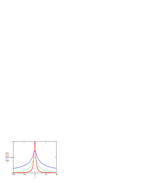
Figure 2: (Color online) Shape of the Josephson current noise spectral lines in the vicinity of the resonances $z=\omega_{\pm}\tau_{\mathrm{GL}}$.

IV Discussions

We have considered effects of superconductive fluctuations on the current noise in tunnel junctions above the critical temperature. Several contributions were identified. The simplest one originates from the fluctuation suppression of the density of states. This effect gives negative contribution to the current noise, which is only logarithmic in temperature $S_{\mathrm{DOS}}\propto\ln(T-T_{c})$, whereas dip in the density of states at the Fermi energy has much stronger temperature dependence $\delta\nu(0)\propto(T-T_{c})^{-2}$. Somehow current and its noise get suppressed weaker than the density of states itself. Another interesting point is that current noise is strongly modified only at the characteristic voltages $eV\sim T_{c}$, while corresponding feature in the density of states appears at energies $\epsilon\sim T-T_{c}$, see Eq. (54). It turns out that higher-order fluctuation effects, similar to that shown in Fig. 1b, restore additional structure of the noise signal at $eV\sim T-T_{c}$. Correction $S_{\mathrm{DOS}}$ is linear in $Gi$ and in tunnel conductance $g_{T}$. This is in contrast to the Josephson current contribution to the noise. The latter is quadratic in fluctuations and in tunneling, and enhances noise at the frequencies in the vicinity of the Josephson frequency $\omega_{J}$. The peak at $\omega=\omega_{J}$ is well defined and is strongly temperature dependent, which makes it possible to detect it experimentally. We have found that depending on the junction configuration: symmetric or non-symmetric and narrow or wide, noise resonance line has different shapes in the frequency domain Fig. 2 and different temperature dependencies.

Closing this section we should mention that in the field of fluctuating superconductivity one usually identifies three types of fluctuation corrections. Apart from density of states, there are also so called Aslamazov-Larkin (AL) and Maki-Thompson (MT) terms mentioned in Sec. I. It is quite natural to ask how AL and MT processes modify current noise and how they can be identified within $\sigma$-model formalism. As an attempt to answer, one should recall that in addition to the simple tunneling term $\mathbb{S}_{T}[V]$, considered in this work, one may have yet another one $i\mathbb{S}_{A}[V]=(\pi g_{A}/16e^{2})\mathrm{Tr}\{\big{(}e^{i\check{\Xi}\check{V}}\check{Q}_{L}e^{-i\check{\Xi}\check{V}}\check{Q}_{R}\big{)}^{2}\}$, which was neglected. It corresponds to Andreev processes, and $g_{A}$ is Andreev conductance. Using $\mathbb{S}_{A}[V]$, instead of $\mathbb{S}_{T}[V]$, one may follow the same routing expanding $\check{Q}$-matrices in fluctuations $\check{W}$ to obtain additional contribution to the noise. However, among all the terms emerging in perturbative expansion, separation on AL and MT contributions becomes ambiguous. Nevertheless, the problem is very interesting and requires further studies.

Many useful discussion with A. Kamenev, M. Reznikov, A. Varlamov and especially G. Catelani are kindly acknowledged. I would like to thank also Digital Material Laboratory at The Institute of Physical and Chemical Research (RIKEN), where this work was finalized, for their hospitality. This work was supported by the NSF Grant No. DMR-0405212 and UMN Graduate School Doctoral Dissertation Fellowship.

V Appendices

V.1 Fluctuations expansion

Within this section we show in details how the transformation from Eq. (II) to Eq. (16) occurs. We start fluctuations expansion by taking $\check{Q}\approx\check{Q}_{N}\big{(}1+i\check{W}-\check{W}^{2}/2\big{)}$ and bringing it into the $\mathbb{S}_{\sigma}$ (here and in what follows subscript $a$ in $\check{Q}_{a}$ matrix and all other elements will be suppressed for brevity). For the trace of the gradient term we find, $\mathrm{Tr}\big{\{}(\nabla\check{Q})^{2}\big{\}}=-\mathrm{Tr}\big{\{}\check{Q}_{N}\nabla\check{W}\check{Q}_{N}\nabla\check{W}\big{\}}=-\mathrm{Tr}\big{\{}\check{\mathcal{W}}\nabla^{2}\check{\mathcal{W}}\big{\}}$, where we employed anti–commutativity relation $[\check{Q}_{N},\check{W}]_{+}=0$ and nonlinear constraint $\check{Q}^{2}_{N}=1$. Using an explicit form of the $\check{\mathcal{W}}$ matrix [Eq. (10)] and tracing the product of two $\check{\mathcal{W}}$ over the Keldysh $\otimes$ Nambu space, we obtain

$$\mathrm{Tr}\left\{(\nabla\check{Q})^{2}\right\}=2\mathrm{Tr}\left\{Dq^{2}\big{[}c^{*}_{\epsilon\epsilon^{\prime}}(q)c_{\epsilon^{\prime}\epsilon}(-q)+\bar{c}^{*}_{\epsilon\epsilon^{\prime}}(q)\bar{c}_{\epsilon^{\prime}\epsilon}(-q)\big{]}\right\}\,.$$ (47)

The time derivative term in the $\mathbb{S}_{\sigma}$ produces contribution $\mathrm{Tr}\big{\{}\check{\Xi}\partial_{t}\check{Q}\big{\}}=\frac{i}{2}\mathrm{Tr}\big{\{}\epsilon\check{R}_{\epsilon}\check{\Xi}\check{R}_{\epsilon}\check{\Lambda}\check{\mathcal{W}}_{\epsilon\epsilon^{\prime}}\check{\mathcal{W}}_{\epsilon^{\prime}\epsilon}\big{\}}$, while linear in $\check{W}$ part traces out to zero [here we used $\check{Q}_{N}(\epsilon)=\check{R}_{\epsilon}\check{\Lambda}\check{R}_{\epsilon}$ with $\check{\Lambda}=\sigma_{z}\otimes\tau_{z}$ and substituted $\partial_{t}\to-i\epsilon$]. Observing that $\check{R}_{\epsilon}\check{\Xi}\check{R}_{\epsilon}\check{\Lambda}=\sigma_{z}\otimes\tau_{0}$, one finds

$$\mathrm{Tr}\left\{\check{\Xi}\partial_{t}\check{Q}\right\}=\frac{i}{2}\mathrm{Tr}\left\{(\epsilon+\epsilon^{\prime})[c^{*}_{\epsilon\epsilon^{\prime}}(q)c_{\epsilon^{\prime}\epsilon}(-q)-\bar{c}^{*}_{\epsilon\epsilon^{\prime}}(q)\bar{c}_{\epsilon^{\prime}\epsilon}(-q)]\right\}.$$ (48)

For the coupling term between Cooperons and $\Delta$, to the leading order, we have $\mathrm{Tr}\big{\{}\check{\Delta}\check{Q}\big{\}}=\mathrm{Tr}\big{\{}\check{R}_{\epsilon}\check{\Delta}_{\epsilon-\epsilon^{\prime}}\check{R}_{\epsilon^{\prime}}\check{\Lambda}\check{\mathcal{W}}_{\epsilon\epsilon^{\prime}}\big{\}}$, which translates into

$$\mathrm{Tr}\big{\{}\check{\Delta}\check{Q}\big{\}}=-i\mathrm{Tr}\left\{[\Delta^{cl}_{\epsilon-\epsilon^{\prime}}(q)+F_{\epsilon}\Delta^{q}_{\epsilon-\epsilon^{\prime}}(q)]c^{*}_{\epsilon^{\prime}\epsilon}(-q)\right.$$ (49)

$$+[\Delta^{*cl}_{\epsilon-\epsilon^{\prime}}(q)+F_{\epsilon}\Delta^{q*}_{\epsilon-\epsilon^{\prime}}(q)]c_{\epsilon^{\prime}\epsilon}(-q)-[\Delta^{cl}_{\epsilon-\epsilon^{\prime}}(q)-$$

$$\left.F_{\epsilon^{\prime}}\Delta^{q}_{\epsilon-\epsilon^{\prime}}(q)]\bar{c}^{*}_{\epsilon^{\prime}\epsilon}(-q)-[\Delta^{*cl}_{\epsilon-\epsilon^{\prime}}(q)-F_{\epsilon^{\prime}}\Delta^{*q}_{\epsilon-\epsilon^{\prime}}(q)]\bar{c}_{\epsilon\epsilon^{\prime}}(-q)\right\}.$$

Combining now Eqs. (47)–(49) all together and bringing them back into the Eq. (II), we wind for the quadratic in Cooperons part of action $\mathbb{S}_{\sigma}[W^{a},\Delta]=\mathbb{S}^{c}_{\sigma}[c,\Delta]+\mathbb{S}^{\bar{c}}_{\sigma}[\bar{c},\Delta]$, where contributions from the retarded $c$ and advanced $\bar{c}$ Cooperons read as

$$i\mathbb{S}^{c}_{\sigma}[c,\Delta]=-\frac{\pi\nu}{2}\mathrm{Tr}\left\{c^{*}_{\epsilon\epsilon^{\prime}}[Dq^{2}-i(\epsilon+\epsilon^{\prime})]c_{\epsilon^{\prime}\epsilon}+2[\Delta^{cl}_{\epsilon-\epsilon^{\prime}}+F_{\epsilon}\Delta^{q}_{\epsilon-\epsilon^{\prime}}]c^{*}_{\epsilon^{\prime}\epsilon}+2[\Delta^{*cl}_{\epsilon-\epsilon^{\prime}}+F_{\epsilon}\Delta^{*q}_{\epsilon-\epsilon^{\prime}}]c_{\epsilon^{\prime}\epsilon}\right\}\,,$$ (50a)

$$i\mathbb{S}^{\bar{c}}_{\sigma}[\bar{c},\Delta]=-\frac{\pi\nu}{2}\mathrm{Tr}\left\{\bar{c}^{*}_{\epsilon\epsilon^{\prime}}[Dq^{2}+i(\epsilon+\epsilon^{\prime})]\bar{c}_{\epsilon^{\prime}\epsilon}-2[\Delta^{cl}_{\epsilon-\epsilon^{\prime}}-F_{\epsilon^{\prime}}\Delta^{q}_{\epsilon-\epsilon^{\prime}}]\bar{c}^{*}_{\epsilon^{\prime}\epsilon}-2[\Delta^{*cl}_{\epsilon-\epsilon^{\prime}}-F_{\epsilon^{\prime}}\Delta^{*q}_{\epsilon-\epsilon^{\prime}}]\bar{c}_{\epsilon^{\prime}\epsilon}\right\}.$$ (50b)

At this stage we are ready to perform integration over the Cooperon modes. Assuming that configuration of the order-parameter field is given, one varies Eq. (50) with respect to $c^{*}$ and $\bar{c}^{*}$, and obtains stationary point equations $\delta\mathbb{S}^{c}_{\sigma}/\delta c^{*}_{\epsilon\epsilon^{\prime}}=0$ and $\delta\mathbb{S}^{\bar{c}}_{\sigma}/\delta\bar{c}^{*}_{\epsilon\epsilon^{\prime}}=0$. The latter are easily solved by Eq. (12). Since the value of the Gaussian integral is equal to that taken at the saddle point, one brings Eq. (12) into Eq. (50) and after some straightforward algebra finds Eq. (16). Further details can be found in Ref. LK, .

V.2 Relation between $S_{\mathrm{DOS}}$ and $\delta\nu(\epsilon)$

The purpose of this section is to demonstrate explicitly that $S_{\mathrm{DOS}}$ indeed originates from the DOS effects, which was hidden in the technical details of Sec. III. To this end we calculate temperature dependence of the $\delta\nu(\epsilon)$ within Keldysh technique. This illustration is useful for the sake of comparison with the known results obtained previously from the temperature Matsubara technique Abrahams .

Within $\sigma$–model energy dependent density of states is expressed in terms of $\check{Q}$ matrix in the following way:

$$\nu(\epsilon)=\frac{\nu}{4}\mathrm{Tr}\big{[}\check{Q}_{N}\check{Q}_{\epsilon\epsilon}\big{]}.$$ (51)

Setting $\check{Q}=\check{Q}_{N}$ one recovers bare normal-metal density of states $\nu(\epsilon)=\nu$. To account for the fluctuations on top of the metallic state, one expands $\check{Q}$ in Cooper modes $\check{W}$ to the quadratic order and averages over $\Delta$ fluctuations with the effective action from Eq. (16);

$$\delta\nu(\epsilon)=-\frac{\nu}{4}\mathrm{Tr}\left[\langle\langle c_{\epsilon\epsilon^{\prime}}(q)c^{*}_{\epsilon^{\prime}\epsilon}(-q)\rangle\rangle+\langle\langle\bar{c}_{\epsilon\epsilon^{\prime}}(q)\bar{c}^{*}_{\epsilon^{\prime}\epsilon}(-q)\rangle\rangle\right].$$ (52)

Observe that this is precisely the same combination of the Cooperons, which enters $S_{\mathrm{DOS}}$ in the Eq. (22), thus they have common origin. Furthermore, it is easy to show that $S_{\mathrm{DOS}}(\omega)\propto\int d\epsilon\,\delta\nu(\epsilon)[F_{\epsilon+u_{\pm}/2T}-F_{\epsilon-u_{\pm}/2T}]$. Using averages from Eq. (III.1), density-of-states correction becomes

$$\frac{\delta\nu(\epsilon)}{\nu}=\mathrm{Im}\sum_{q}\int^{+\infty}_{-\infty}\frac{d\omega}{2\pi}\frac{\mathcal{L}_{K}(q,\omega)+F_{\epsilon}\mathcal{L}_{R}(q,\omega)}{(Dq^{2}-2i\epsilon+i\omega)^{2}}.$$ (53)

where we set $\epsilon^{\prime}=\epsilon-\omega$. Here one meets the convenience of the Keldysh technique, which allows us to get physical quantities avoiding analytic continuation procedure. Using explicit form of fluctuations propagators from Eq. (18) and performing frequency and momentum integrations, one finds in the quasi–two–dimensional case,

$$\frac{\delta\nu(\epsilon)}{\nu}=-\frac{Gi}{16}\left(\frac{T_{c}}{T-T_{c}}\right)^{2}\mathcal{F}(\epsilon\tau_{\mathrm{GL}}),$$ (54a)

where dimensionless function is

$$\mathcal{F}(z)=\mathrm{Re}\int^{+\infty}_{0}\frac{dx}{(1+x)(1+2x-2iz)^{2}}\,.$$ (54b)

In agreement with Ref. [Abrahams, ] dip at the Fermi energy is $\delta\nu(0)\propto(T-T_{c})^{-2}$, while at large energies $\epsilon\tau_{\mathrm{GL}}\gg 1$ density-of-states correction recovers its normal value according to $\delta\nu(\epsilon)\propto(T_{c}/\epsilon)^{2}\ln(\epsilon\tau_{\mathrm{GL}})$.

V.3 Integrals for $S_{\mathrm{DOS}}(\omega)$ and $S_{J}(\omega)$

(I) Transformation from Eq. (26) to Eq. (III.1) requires calculation of the integral,

$$I=\int^{+\infty}_{0}dx\iint^{+\infty}_{-\infty}dydz\,\mathrm{Re}\frac{F_{z+u_{\pm}/2T}-F_{z-u_{\pm}/2T}}{\big{[}(x+\eta)^{2}+y^{2}\big{]}(x+iy-4iz)^{2}}.$$ (55)

One performs $y$ integration first,

$$I=\pi\int^{+\infty}_{0}dx\int^{+\infty}_{-\infty}dz\,\mathrm{Re}\frac{F_{z+u_{\pm}/2T}-F_{z-u_{\pm}/2T}}{(x+\eta)(\eta+2x-4iz)^{2}}.$$ (56)

Since $\eta\ll 1$ and relevant $z\sim 1$ one may safely approximate $(\eta+2x-4iz)\approx 2(x-2iz)$. Then expanding $F_{z}$ into the series $F_{z}=2\sum_{n}z/(z^{2}+z^{2}_{n})$, with $z_{n}=\pi(n+1/2)$, interchanging order of summation and integration and recalling definition of the $n$th–order derivative of the digamma function $\psi^{[n]}(z)=(-1)^{n+1}n!\sum^{\infty}_{n=0}1/(n+z)^{n+1}$, one finds that

$$\int^{+\infty}_{-\infty}dz\frac{F_{z\pm u_{\pm}/2T}}{(x-2iz)^{2}}=\frac{i}{2\pi}\psi^{[1]}\left(\frac{1}{2}\pm\frac{iu_{\pm}}{2\pi T}+\frac{x}{2\pi}\right).$$ (57)

Remaining $x$ integration can be taken with logarithmic accuracy, ignoring $x$ dependence of the digamma function since only $x\lesssim 1$ contribute significantly, which eventually gives $-\ln\eta$. Combining all together, one finds

$$I=\frac{1}{4}\ln(1/\eta)\mathrm{Im}\psi^{[1]}\left(\frac{1}{2}-\frac{iu_{\pm}}{2\pi T}\right)\,,$$ (58)

which in combination with Eq. (26) results in Eq. (III.1).

(II) Transition from Eq. (38) to Eq. (39) is performed in the following way. As the first step one finds Keldysh component of the fluctuation propagator in the mixed momentum/time representation $\mathcal{L}_{K}(q,t)=\int\mathcal{L}_{K}(q,\omega)e^{-i\omega t}d\omega/2\pi$, which gives

$$\mathcal{L}_{K}(q,t)=-\frac{2iT^{2}_{c}}{T-T_{c}}\frac{e^{-\varkappa_{q}|t|/\tau_{\mathrm{GL}}}}{\varkappa_{q}},\quad\varkappa_{q}=(\xi_{\mathrm{GL}}q)^{2}+1.$$ (59)

One inserts then $\mathcal{L}_{K}(r,t)=\int\mathcal{L}_{K}(q,t)e^{iqr}dq^{2}/4\pi$ into Eq. (38), integrates over $r$, introduces dimensionless time $\tau=t/\tau_{\mathrm{GL}}$, and changes from $q$ to $\varkappa$ integration $dq^{2}=d\varkappa/\xi^{2}_{\mathrm{GL}}$, which gives all together

$$S_{J}(\omega)=\sum_{\pm}\frac{\pi Gi^{2}}{64T_{c}}\left(\frac{g_{T}T_{c}}{e}\right)^{2}\frac{\xi^{2}_{o}}{\mathcal{A}}\left(\frac{T_{c}}{T-T_{c}}\right)^{2}\qquad\qquad$$

$$\times\int^{+\infty}_{-\infty}d\tau\int^{+\infty}_{1}\frac{d\varkappa}{\varkappa^{2}}e^{-2\varkappa|\tau|-iz_{\pm}\tau}\,,$$ (60)

where $z_{\pm}=\omega_{\pm}\tau_{\mathrm{GL}}$. After $\tau$ integration one is left with

$$\int^{\infty}_{1}\frac{4d\varkappa}{\varkappa(4\varkappa^{2}+z^{2}_{\pm})}\,,$$ (61)

which defines $N(z)$ function in Eq. (39).

(III) Calculation of Eq. (III.2) is completely analogous. Noticing that $\mathcal{L}_{K}(0,t)=\int\mathcal{L}_{K}(q,t)dq^{2}/4\pi$ and transforming to the dimensionless units $\tau=t/\tau_{\mathrm{GL}}$ and $\varkappa=(\xi_{\mathrm{GL}}q)^{2}+1$, we have

$$S_{J}(\omega)=\sum_{\pm}\frac{Gi^{2}\tau_{GL}}{4\pi^{2}}\left(\frac{g_{T}T_{c}}{e}\right)^{2}\qquad\qquad\qquad$$

$$\times\int^{+\infty}_{-\infty}d\tau\iint^{+\infty}_{1}\frac{d\varkappa d\varkappa^{\prime}}{\varkappa\varkappa^{\prime}}e^{-(\varkappa+\varkappa^{\prime})|\tau|-iz_{\pm}\tau}.$$ (62)

After $\tau$ integration one is left with

$$\iint^{+\infty}_{1}\frac{d\varkappa d\varkappa^{\prime}}{\varkappa\varkappa^{\prime}}\frac{\varkappa+\varkappa^{\prime}}{(\varkappa+\varkappa^{\prime})^{2}+z^{2}_{\pm}}=\frac{2}{z_{\pm}}\int^{+\infty}_{1}\frac{d\varkappa}{\varkappa}\mathrm{arccot}\left(\frac{1+\varkappa}{z_{\pm}}\right)$$ (63)

which after the integration by parts reduces to $2M(z)$, with $M(z)$ function defined by Eq. (III.2).

References

• (1) A. I. Larkin and A. Varlamov, Theory of Fluctuations in Superconductors (Clarendon, Oxford, 2005).
• (2) L. G. Aslamazov and A. I. Larkin, Fiz. Tverd. Tela 10, 1104 (1968) [Sov. Phys. Solid. State 10, 875 (1968)].
• (3) K. Maki, Prog. Theor. Phys. 39, 897 (1968).
• (4) I. O. Kulik, Pis’ma Zh. Eksp. Teor. Fiz. 10, 488 (1969) [Sov. Phys. JETP Lett. 10, 313 (1969)].
• (5) D. J. Scalapino, Phys. Rev. Lett. 24, 1052 (1970).
• (6) A. Varlamov, G. Balestrino, E. Milani and D. V. Livanov, Adv. Phys. 48, 655 (1999).
• (7) I. Martin and A. Balatsky, Phys. Rev. B 62, R6124 (2000).
• (8) Xi Dai, Tao Xiang, Tai Kai Ng and Zhao-bin Su, Phys. Rev. Lett. 85, 3009 (2000).
• (9) V. V. Dorin and M. V. Fistul’, Phys. Rev. B 46, 13951 (1992).
• (10) E. Shimshoni, P. M. Goldbart and N. Goldenfeld, Phys. Rev. B 48, 9865 (1993).
• (11) M. Reznikov, private communications.
• (12) A. Kamenev and A. Andreev, Phys. Rev. B 60, 2218 (1999).
• (13) M. V. Feigel’man, A. I. Larkin and M. A. Skvortsov, Phys. Rev. B 61, 12361 (2000).
• (14) A. Kamenev, in Nanophysics: Coherence and Transport, edited by H.Bouchiat et. al. (Elsevier, New York, 2005), p. 177.
• (15) A. Levchenko and A. Kamenev, Phys. Rev. B, 76, 094518 (2007).
• (16) E. Abrahams, M. Redi, and J. W. Woo, Phys. Rev. B 1, 208 (1970).
• (17) A. A. Varlamov and V. V. Dorin, Zh. Eksp. Teor. Fiz. 84, 1868 (1983) [Sov. Phys. JETP 57, 1089 (1983)].
• (18) Here additional subscript $R$ in the notations of matrix $\check{W}^{R}$ was suppressed for brevity. According to the assumption $\check{W}^{L}=0$ for the non-symmetric configuration.
• (19) Deriving Eq. (32) we have ignored quantum component of the order parameter $\Delta^{q}(r,t)$. Although formaly present it gives at the end subleading contribution to the noise spectrum.